Caloric curves of atomic nuclei and other small systems
Abstract
Caloric curves have traditionally been derived within the microcanonical ensemble via or within the canonical ensemble via . In the thermodynamical limit, i.e., for large systems, both caloric curves give the same result. For small systems like nuclei, the two caloric curves are in general different from each other and neither one is reasonable. Using , spurious structures like negative temperatures and negative heat capacities can occur and have indeed been discussed in the literature. Using a very featureless caloric curve is obtained which generally smoothes too much over structural changes in the system. A new approach for caloric curves based on the two-dimensional probability distribution will be discussed.
PACS number(s): 05.20.Gg, 05.70.Fh, 21.10.Ma, 24.10.Pa
I Introduction
A common misconception in phenomenological thermodynamics is the notion that the caloric curve is given by
| (1) |
in the microcanonical ensemble, and by
| (2) |
in the canonical ensemble.†††Throughout this work we will set the Boltzmann constant . This is only true in the thermodynamical limit, where both caloric curves coincide, but it is certainly not true for small systems like atomic nuclei where the two curves can differ dramatically from each other [1].
Closely connected with this error is the believe that the temperature in the microcanonical ensemble is defined by Eq. (1). At this point, we would therefore like to emphasize that the temperature scale is defined by the triple point of water and several secondary standards. Temperatures themselves are defined by a measurement process, i.e., by a comparison of an unknown temperature to temperature standards. Since this measurement process requires the exchange of energy between the system under study and a thermometer, we can immediately see that the concept of a temperature can conflict with the concept of a microcanonical ensemble which is, per definition, closed for energy exchange. The solution to this problem for large system is the incorporation of a relatively small thermometer into the microcanonical system. Only for this case it has been shown experimentally that the definition of the temperature coincides with Eq. (1). For a small microcanonical system, no such solution exists and the temperature of such a system has to remain undefined, since it cannot be measured. Therefore, for any small system, temperature has always to be introduced by a coupling of the system under study to a large heat bath.
II Traditional caloric curves
As starting point for the discussion in this work, we take the probability of a system to have the energy for a given temperature which is imposed by a large heat bath
| (3) |
Here, is the multiplicity of states with energy , and is the canonical partition function
| (4) |
In the derivation of this probability distribution, one usually takes advantage of Eq. (1) applied to the heat bath. Since the heat bath is thought to be approximately in the thermodynamical limit, the use of Eq. (1) is justified and will not conflict with our claim in the present work that for small systems, Eq. (1) will become unphysical.
Now, for convenience, it is often easier to use the logarithm of the probability than the probability itself. We therefore define
| (5) |
In the thermodynamical limit, for a given , the most probable value of which we will denote throughout this work is determined by the condition
| (6) |
Simple algebra shows that this condition is equivalent to
| (7) |
where is the microcanonical entropy. Here, we have recovered the traditional expression for the caloric curve in the microcanonical ensemble. However, a word of caution is necessary: for small systems, the above condition does not necessarily give always the most probable value , but can, under certain circumstances, yield the locally least probable value of , denoted . We will later give an example for this claim. It is only in the thermodynamical limit that always the most probable value of is obtained. In this limit, the construction of the microcanonical caloric curve is therefore equivalent to finding for a given .
Alternatively, we can search for the most probable value of (denoted ) for a given . In the thermodynamical limit, this value is obtained through the condition
| (8) |
which is equivalent to
| (9) |
Here, we have recovered the traditional expression for the caloric curve in the canonical ensemble.
Let us now calculate the average energy
| (10) |
of the distribution for a given temperature . Again, simple algebra yields
| (11) |
which is the same result as before. This means that the construction of the canonical caloric curve is equivalent to:
-
finding for a given temperature
-
finding for a given energy .
The first feature makes the canonical curve more robust and therefore more attractive than the microcanonical curve.
In general, caloric curves are constructed by replacing the distribution of energies (temperatures) for a given temperature (energy) by a special value of this distribution, often the most probable value or the mean value. This gives satisfactory results in the thermodynamical limit, where the distributions are very sharp, almost -like, and where therefore the mean value and the most probable value will coincide. This causes also that the traditional microcanonical and canonical caloric curves coincide in the thermodynamical limit. For small systems, however, the probability distribution can be quite flat and exhibit more than one maximum. Thus, a one-by-one relation of temperature and energy as represented by a caloric curve can only serve as an approximate concept. Further, as shown above, the approximations in deriving a caloric curve for small systems are manifested differently in the microcanonical and canonical ensemble, i.e. by finding (or sometimes ) for a given in the microcanonical ensemble or by finding for a given in the canonical ensemble (or alternatively, by finding for a given ). Thus, the two resulting caloric curves can, in general, be vastly different for the same (small) system.
The physical reason behind the inherently approximative nature of the concept of caloric curves for a small system is the Laplace transformation which connects the two statistical ensembles as shown in Eq. (4). From a mathematical point of view, this transformation is not unlike the Fourier transformation connecting the coordinate and momentum space in quantum mechanics. In analogy to quantum mechanics, we can therefore regard the microcanonical ensemble as the ’energy representation’ of the system, since the control parameter is the energy, while the temperature is fluctuating. The canonical ensemble can then be regarded as the ’temperature representation’, since here, the temperature is the control parameter while the energy is fluctuating. Further, just as the exact knowledge of momentum (or coordinate) implies, according to Heisenberg, large uncertainties in the other quantity, in thermodynamics of small systems, a fixed value of (imposed by a heat bath) implies large fluctuations in , and a fixed (as in the microcanonical ensemble) implies an ill-defined due to fluctuations. Only in the thermodynamical limit, the relative fluctuations will become negligibly small and the caloric curve will again become an exact concept, just as in classical mechanics, an object can again have a definite coordinate and momentum.
Acknowledging the approximative nature of the concept of caloric curves, we will, in the following, show that in general neither the microcanonical nor the canonical ensemble actually gives a good approximation for the caloric curve. Therefore, a new method will be proposed to construct more meaningful caloric curves for small systems.
III Shortcomings of traditional caloric curves in small systems
First, we will investigate a simple example where the multiplicity of states is proportional to . Simple algebra shows that the microcanonical caloric curve is given by
| (12) |
whereas the canonical caloric curve is given by
| (13) |
Figure 1 shows together with the two traditional caloric curves for the case . Obviously, the two curves do not coincide and neither seems to represent a good characterization to the probability distribution . In this example, the thermodynamical limit is approached by increasing . Figure 2 gives the case for where both approaches yield more similar curves and the collapse of the probability distribution into a caloric curve becomes a better approximation, mainly because exhibits much sharper maxima as function of or . As a third example, we take a simple Fermi-gas level-density expression
| (14) |
which gives the usual
| (15) |
in the microcanonical ensemble, and the less used, but more accurate
| (16) |
with
| (17) |
in the canonical ensemble‡‡‡For large , this expression simplifies to , for small (i.e., large ), one obtains . (see Fig. 3). An actual example for caloric curves from a system which exhibits approximately a Fermi-gas level density is given in Fig. 4.
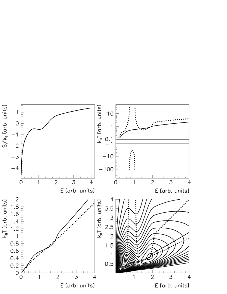
An interesting example is obtained when a convex intruder is present in the microcanonical entropy curve. Such a structure is only possible for finite systems since for infinite systems, the second law of thermodynamics requires a concave entropy as function of energy. In the literature, such structures have been discussed, e.g., for the melting of atomic clusters [2], fragmentation of nuclei [3], and large composite systems like star clusters [4]. Figure 5 gives an example with a relatively weak dip in the entropy curve. For this example, the microcanonical caloric curve lies always above the canonical caloric curve. In the next example (see Fig. 6), the dip in the entropy curve is made larger, such that the microcanonical and canonical caloric curves cross each other at two points. At the two crossing points the probability distribution has a saddlepoint and a local maximum, respectively. However, in general, also here the microcanonical caloric curve lies mostly above the canonical caloric curve, in agreement with experimental observations [1]. Figure 7 gives an example of an atomic nucleus where the logarithmic level density has several convex regions. Those convex intruders indeed cause the microcanonical and canonical caloric curves to cross several times. The structural changes in the 172Yb nucleus which cause the convex regions in the microcanonical entropy curve in the first place are thought to be the breakup of nucleon Cooper pairs [1, 6].
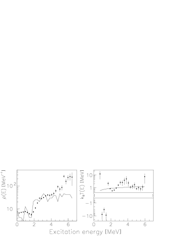
Finally, the dip can be made so large that the entropy locally decreases with increasing energy (see Fig. 8). This means that the probability distribution for all large enough exhibits at least two local maxima (and in many cases a local minimum in between), a phenomenon not uncommon for small (especially discrete) systems. The negative branch of the microcanonical caloric curve is again an unphysical structure induced by the attempt to characterize the probability distribution for a fixed by an extremum of . Also this extreme case has been observed in the experimental level density of the 57Fe nucleus [8] (see Fig. 9). The physical origin of the local decrease in the level density of 57Fe is probably simply a fluctuation in the level spacing. The sharp increase in level density above 2 MeV excitation energy has again been attributed to the breaking of proton Cooper pairs [5].
Until now, the emphasis has been on the unphysical results one obtains when using the microcanonical caloric curve. However, also the canonical caloric curve does not capture the thermodynamics of the systems under study correctly. In general, the canonical caloric curve smoothes too much over structural changes and remains always featureless, which makes it rather unattractive (see Figs. 5–9). To overcome this problem, its derivative, the canonical heat capacity
| (18) |
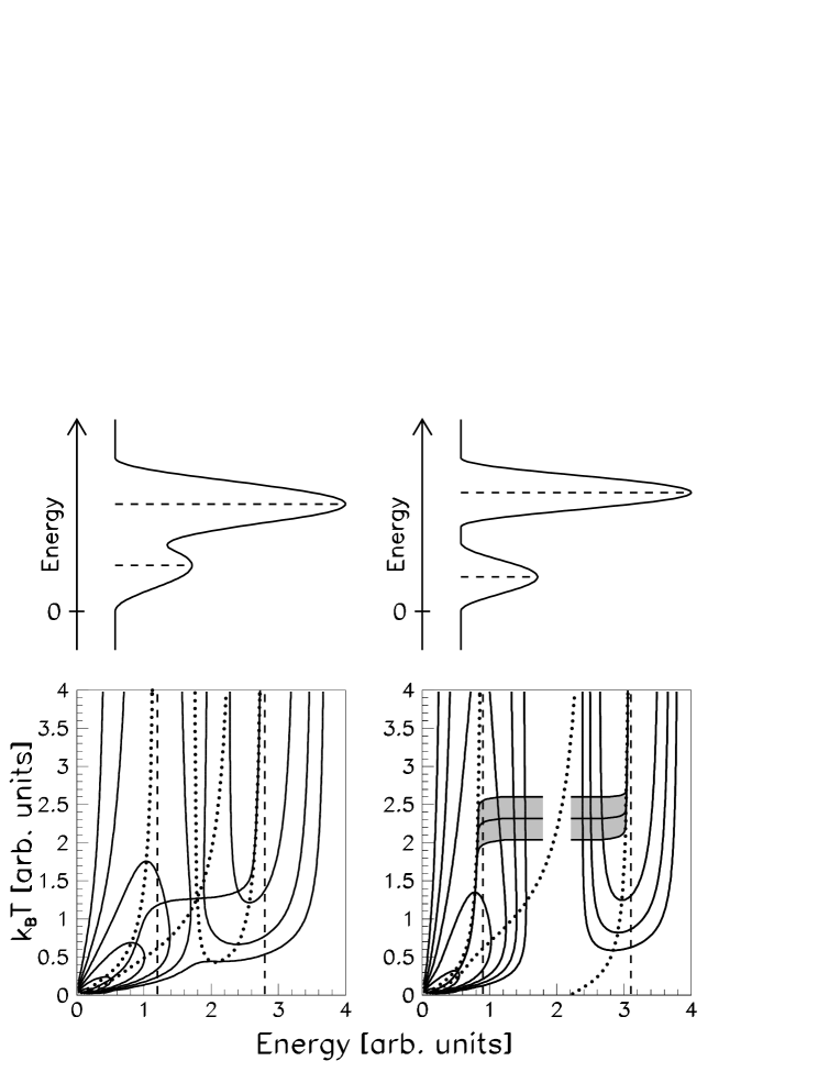
has been used with success to characterize structural changes in real nuclei, like the quenching of pairing correlations as function of temperature [6, 10, 11]. The lack of features in the canonical caloric curve becomes even clearer for the more extreme examples described in Fig. 10. There, a two-level system is discussed where the degeneracy of the upper level is thrice the degeneracy of the lower level. One could, e.g., think of the two levels as a spin 0 ground state and a spin 1 excited state.§§§For the present model of a two-level system, there is no real corresponding example from nuclear physics. However, one can easily imagine that a similar system could actually be realized in, e.g., atomic physics. For the sake of the discussion, a width has been given to both levels such that the two levels do (upper left-hand panel) or do not (upper right-hand panel) overlap. The probability distributions are centered around the level energies and . While the microcanonical curve is again multivalued and exhibits negative branches (not shown in the figure), the canonical caloric curve is smooth and reaches the value of for infinite temperatures. Evident from the figure is the fact that at temperatures around for the lower left-hand panel and for the lower right-hand panel, the probability for the particle to be located in the lower or upper level becomes approximately equal. The canonical caloric curve now still connects locations with vertical tangents of the contour lines, i.e., it describes for a given the system by the most probable value . On the other hand, as can be seen in the lower panels of Fig. 10, for energies which are rather improbable (left-hand side) or simply cannot be realized by the system like –2.2 (right-hand side), this feature does not make sense. Neither does the other feature of the canonical caloric curve make sense, i.e., to describe the system by its average energy for a given , as long as coincides with values close to the locally least probable value (lower left-hand panel) or to a completely impossible value of (lower right-hand panel). The canonical caloric curve simply dwells for a too long temperature region in the vicinity of improbable or impossible values of .
IV New caloric curve
It is now an interesting question how to define a caloric curve for a small system which can overcome all of these problems. In general, the system has of course always to be described by the probability distribution, since is most often flat and can exhibit more than one maximum. Therefore, the distribution cannot be collapsed to one special value without loosing some of the dynamics. On the other hand, caloric curves have been very useful for large systems and it might prove fruitful to extend the concept of a caloric curve to small systems as well. The only obvious guidelines for constructing a caloric curve is now that it should coincide in the thermodynamical limit to the traditional constructions of a caloric curve and that it does, at no point (or at as few points as possible), collapse the probability distribution to a locally least probable value (or to a value close to a locally least probable value).
Obviously, one could imagine many different possibilities to define a caloric curve for small systems which will fulfill the abovementioned conditions. In this sense, the approach chosen in this work is certainly not unique, and it can be discussed whether it is the best choice for all cases. Our intuitive assumptions for the construction of a new caloric curve come from a close inspections of Figs. 1 and 2. There, we see that for increasing values of (which corresponds to approaching the thermodynamical limit), the curves of constant probability become more and more pointed and the points with horizontal and vertical tangents move closer together. Our feeling is therefore, that an appropriate ’mean’ caloric curve is the curve which always lies in between the two traditional caloric curves and crosses the contour curves of equal probability perpendicularly. Now, the contour curves of constant probability are characterized by the differential equation
| (19) |
The curves perpendicular to those contour curves have a first derivative which is the negative inverse of the first derivative of the contour curves and are thus given by
| (20) |
which is equivalent to the differential equation
| (21) |
This equation describes all (infinitely many) curves which perpendicularly cross the contour curves of equal probability (one of them is given as the dash-dotted line in Fig. 1), and we therefore have to introduce the second part of our assumption in order to single out one solution: the new caloric curve should always lie between the two traditional caloric curves. This is mathematically done by looking at the asymptotic behavior of the curves described by Eq. (21). The solid lines in Figs. 1–3 are such curves. They are in general closer to the canonical caloric curves, which supports our claim that Eq. (16) is a better representation of the nuclear temperature than Eq. (15), and do not show any surprising features.
The solid line in Fig. 5 in the lower right-hand panel is also a solution of Eq. (21) with the correct asymptotic behavior. Again, the new caloric curve is rather close to the canonical caloric curve, but it shows clearly more features (reflecting the structural change of the system under study, which is modeled by the convex entropy intruder). Of course, these features could again be amplified by taking the derivative of the caloric curve, i.e., the heat capacity, as has been done for the canonical caloric curve. In Figs. 6 and 8, the two traditional caloric curves actually cross, and the condition that the new caloric curve should always lie in between the two traditional caloric curves imposes that the new caloric curve also goes through the two crossing points. From a mathematical point of view, it is now easier to calculate the new caloric curve starting from the saddlepoint of the probability distribution, going in both directions. The new caloric curve beyond the local maximum in the probability distribution, however, is still determined by the correct asymptotic behavior. Obviously, the features in the new caloric curve become more visible the larger the convex intruder in the entropy becomes. Also, the features are always more pronounced than in the canonical caloric curve. On the other hand, the new caloric curve avoids spurious structures like negative heat capacities (i.e. ’backbending’) and branches of negative temperatures, which have been puzzling and often led to claims of first-order phase transitions in small systems.
Unfortunately, the quality of our experimental data on nuclear level densities does not allow us to compute the new caloric curve according to Eq. (21). The main problem is the large granularity of the data, i.e., the binning into 120 keV broad excitation energy intervals. Also, the error bars of the logarithmic nuclear level density are not sufficiently small in order to determine its first derivative with good enough accuracy, as can already be seen for the experimental microcanonical caloric curves.
Finally, the lower left-hand panel of Fig. 10 shows that the new caloric curve tends to avoid the region of improbable values of for a given by sweeping fast from to the within a very small temperature interval. This is also an example where the new caloric curve for most values of actually comes closer to the microcanonical caloric curve than to the canonical caloric curve. The asymptotic behavior of the new caloric curve in Fig. 10 is not an issue, since the integration of Eq. (21) starts at the saddlepoint, and no local maximum of the probability distribution exists. In the lower right-hand panel of Fig. 10, even the saddlepoint in the probability distribution is not well defined, since it depends strongly on the details of the tails of the two levels under consideration. Thus, it is harder to uniquely define the new caloric curve. If one simply cuts off the tails at some energy, (between 1.8 and 2.2 in the example), the saddlepoint is completely undefined and the new caloric curve has to jump from the lower cut-off energy to the higher cut-off energy at a somewhat arbitrary temperature. Although, at a first glance, such a behavior might imply a first-order phase transition, this is not necessarily the case, since additional requirements for the occurrence of a phase-transition-like phenomenon in a small system have to be fulfilled [12, 13, 14]. For the sake of the discussion, we have calculated several new caloric curves starting all at the cut-off energies but with different initial values of the temperature. It can be seen that all curves approach the microcanonical caloric curve in the most direct manner and then follow it down to zero or up to infinite temperature. Thus, while the qualitative features of the new caloric curve are equal for all reasonable initial temperatures, the actual transition temperature (where the new caloric curve sweeps from to ) is rather undefined and depends strongly on the details of the tails of the two levels under consideration. This fact is reflected by the grey-shaded area of Fig. 10 which covers most of the area where reasonably the new caloric curve could be expected.
V Conclusions
It has been shown that traditional caloric curves often fail to capture the thermodynamics of small systems and describe systems in large regions by locally least or even completely impossible values of the energy for a given temperature. A different construction for caloric curves in small systems has been proposed which mostly omits these drawbacks. Thus, spurious structures like negative temperatures and negative heat capacities which are often seen in the microcanonical caloric curves disappear, but on the other hand, more structures in the new caloric curve are evident than in the usually featureless canonical caloric curves. Although the newly proposed construction of caloric curves is just that, a construction, it will be interesting to investigate whether the more pronounced features of the new caloric curves can be related to phase-transition-like phenomena in small systems in a similar way as it has been done for the traditional caloric curves in the thermodynamical limit. The proposed construction of caloric curves can be applied to study the breaking of nucleon Cooper pairs where complete level-density information is available. It could also be applied for other problems in nuclear physics, e.g., in the analysis of multifragmentation data or in the search for the transition to the quark-gluon plasma. It is also conceivable that the use of the new caloric curves is not limited to atomic nuclei alone, but that it might be applied to other small systems in other branches of physics as well.
ACKNOWLEDGMENTS
Part of this work was performed under the auspices of the U.S. Department of Energy by the University of California, Lawrence Livermore National Laboratory under Contract No. W-7405-ENG-48. Financial support from the Norwegian Research Council (NFR) is gratefully acknowledged. We would like to thank E. Tavukcu for carrying out some preliminary calculations for this work. One of us (A.S.) would like to thank Ben Mottelson, Luciano Moretto and Larry Phair for interesting discussions.
REFERENCES
- [1] E. Melby, L. Bergholt, M. Guttormsen, M. Hjorth-Jensen, F. Ingebretsen, S. Messelt, J. Rekstad, A. Schiller, S. Siem, and S. W. Ødegård, Phys. Rev. Lett. 83, 3150 (1999).
- [2] Martin Schmidt, Robert Kusche, Thomas Hippler, Jörn Donges, Werner Kronmüller, Bernd von Issendorff, and Hellmut Haberland, Phys. Rev. Lett. 86, 1191 (2001).
- [3] D.H.E. Gross, Phys. Rep. 279, 119 (1997).
- [4] W. Thirring, Z. Phys. 235, 339 (1970).
- [5] A. Schiller et al., nucl-ex/0302028.
- [6] A. Schiller, A. Bjerve, M. Guttormsen, M. Hjorth-Jensen, F. Ingebretsen, E. Melby, S. Messelt, J. Rekstad, S. Siem, and S. W. Ødegård, Phys. Rev. C 63, 021306(R) (1999).
- [7] A. Voinov, M. Guttormsen, E. Melby, J. Rekstad, A. Schiller, and S. Siem, Phys. Rev. C 63, 044313 (2001).
- [8] E. Tavukcu, Ph.D. thesis, North Carolina State University, 2002.
- [9] R.B. Firestone and V.S. Shirley, Table of Isotopes, 8th ed. (Wiley, New York, 1996), Vol. I.
- [10] S. Liu and Y. Alhassid, Phys. Rev. Lett. 87, 022501 (2001).
- [11] J.L. Egido, L.M. Robledo, and V. Martin, Phys. Rev. Lett. 85, 26 (2000).
- [12] Peter Borrmann, Oliver Mülken, and Jens Harting, Phys. Rev. Lett. 84, 2000.
- [13] A. Schiller, M. Guttormsen, M. Hjorth-Jensen, J. Rekstad, and S. Siem, Phys. Rev. C 66, 024322 (2002).
- [14] M. Guttormsen, R. Chankova, M. Hjorth-Jensen, J. Rekstad, S. Siem, A. Schiller, and D. Dean, nucl-ex/0209013.