An algebraic solution of the multichannel problem applied to low energy nucleon-nucleus scattering

Abstract

Compound resonances in nucleon-nucleus scattering are related to the discrete spectrum of the target. Such resonances can be studied in a unified and general framework by a scattering model that uses sturmian expansions of postulated multichannel interactions between the colliding nuclei. Associated with such expanded multichannel interactions are algebraic multichannel scattering matrices. The matrix structure of the inherent Green functions not only facilitates extraction of the sub-threshold (compound nucleus) bound state spin-parity values and energies but also readily gives the energies and widths of resonances in the scattering regime. We exploited also the ability of the sturmian-expansion method to deal with non-local interactions to take into account the strong non-local effects introduced by the Pauli principle. As an example, we have used the collective model (to second order) to define a multichannel potential matrix for low energy neutron-¹²C scattering allowing coupling between the $0^{+}_{1}$ (ground), $2^{+}_{1}$ (4.4389 MeV), and $0^{+}_{2}$ (7.64 MeV) states. The algebraic $S$ matrix for this system has been evaluated and the sub-threshold bound states as well as cross sections and polarizations as functions of energy are predicted. The results are reflected in the actual measured data, and are shown to be consistent with expectations as may be based upon a shell model description of the target and of the compound nucleus.

I Introduction

Predicting the scattering of low energy (E $<$ 10 MeV) protons and neutrons from nuclei is of wide-spread interest, as is their capture by same. Intrinsically, the probabilities of reactions (measured cross-section data) reflect the inherent structure and modes of excitation of the struck nucleus. However, despite the large amount of data so far accrued, there remains much that has not been measured, or cannot be, but the knowledge of which is prime input to many fields of study; fields as diverse as nuclear-astrophysics/cosmology and nuclear stockpile stewardship.

The most commonly studied process (experimentally and theoretically) is that of elastic scattering; the outcome of such data analysis generally being required to begin studies of other reaction processes. Typically, low-energy elastic scattering data show resonances upon a smoothly varying background, with cross-section magnitudes of the order of barns. Resonances can be quite varied in their character. Particularly their widths (full widths at half maximum, FWHM) vary from a few eV to over an MeV. For light mass targets the resonances in the low energy regime tend to be distinct and but a few in number. As mass increases, however, the numbers of resonances rapidly increase and the first tends lower in energy. Many strongly overlap, so that a statistical approach to the analysis of scattering becomes feasible and utilitarian. But in the main, data analysis to date has been phenomenological, with many parameter values obtained by a fitting process. Little can be interpreted thereby about the intrinsic nature of the target, and the associated theory cannot be made predictive for estimations of the unmeasured (or unmeasurable) cross sections as needed in many other studies. That is also the case with many applications of $R$-matrix theory of scattering Lane and Robson (1966), though at least one Rikus and Amos (1980), for n-¹²C scattering, sought to specify the background scattering from an optical potential with partial widths of the resonances specified from ($p$-$s$-$d$) basis shell-model wave functions of the nuclei involved, i.e. ^12,13C.

However, a more promising multichannel coupling theory of the scattering of neutrons from nuclei has been developed by the Padova group Pisent and Canton (1986); Canton et al. (1987, 1988); Cattapan et al. (1990, 1991); Pisent and Svenne (1995); a theory based upon the work of Rawitscher and Delic Rawitscher (1982); Rawitscher and Delic (1984). The approach is predicated upon making finite-rank separable representations of realistic interaction potentials and the properties of scattering matrices for such Schrödinger interactions.

In brief, the approach starts with auxiliary sturmian functions (Weinberg states) forming a basis set in the interaction region. Initially one chooses a solvable potential problem at any suitable fixed negative energy from which first generation sturmians can be specified in closed analytic form. Second generation sturmians built upon the putative interaction potential matrices for a multichannel scattering problem of interest then can be found as linear combinations of that first generation set. The essential expansion coefficients result from a matrix diagonalization process.

The scheme enables expansions (usually truncated to finite rank for numerical application) of the chosen interaction potentials in terms of those second generation sturmians, each in the form of a sum of separable interactions. The analytic properties of the scattering matrix from a separable Schrödinger potential gives the means by which a full algebraic solution of the multichannel scattering problem can be realized. Of note is that the algebraic structure of the Green functions, that lie at the heart of the $S$ matrices, facilitates the identification of all resonances. The spin-parity ($J^{\pi}$), centroid, and width of each resonance can be ascertained without the need of a super-fine grid of energy values. It is important to identify especially narrow resonances that the scattering model predicts.

The multichannel formalism is outlined next in Sec. II. In this section there are two subsections, in the first of which we give some details of separable representations of potential matrices in terms of sturmian functions. In the second subsection, the process by which we can identify and locate resonances is described. The potential matrices specified using the Tamura collective model of scattering Tamura (1965) then are discussed in Sec. III. This section also outlines how we deal with the Pauli principle, using orthogonalizing pseudo-potentials. Results of calculations in which deformation of that collective model for interaction potential matrices has been taken to second order in the case of neutron scattering from ¹²C allowing coupling to the $0^{+}_{1}$ (ground), $2^{+}_{1}$ (4.4389 MeV), and $0^{+}_{2}$ (7.64 MeV) states, and found for neutron (laboratory) energies to 5 MeV, are presented and discussed in Sec. IV. Note that we use laboratory frame energies when dealing with the scattering domain as the data to be used is so specified. However, when considering the bound states (below the n-¹²C threshold) and/or spectra of ¹³C we use energies in the center of mass system as such are used in tabulations of that spectra Ajzenberg-Selove (1991).

But the collective model of nuclear structure is limited in scope and eventually we shall use this algebraic approach with microscopic (shell) model specifications of the target nuclei providing structure information which, when folded with an effective two-nucleon force, will determine the base input nucleon-nucleus potential matrices. That such shell model structures are reasonable for this purpose, at least with light mass targets, is considered finally in Sect. V.

II The multichannel $T$ matrix from separable interactions

Consider a system of $C$ channels for each allowed scattering spin-parity $J^{\pi}$ with the index $c\ (=1,C)$ denoting the quantum numbers that identify each channel uniquely. Suppose $c=1$ designates the elastic channel. The integral equation approach in momentum space for potential matrices $V_{cc^{\prime}}^{J^{\pi}}(p,q)$, requires solution of coupled Lippmann-Schwinger (LS) equations giving a multichannel $T$ matrix of the form

$$T_{cc^{\prime}}^{J^{\pi}}(p,q;E)=V_{cc^{\prime}}^{J^{\pi}}(p,q) + \mu\left[\sum_{c^{\prime\prime}=1}^{\rm open}\int_{0}^{\infty}V_{cc^{\prime\prime}}^{J^{\pi}}(p,x)\frac{x^{2}}{k^{2}_{c^{\prime\prime}}-x^{2}+i\epsilon}T_{c^{\prime\prime}c^{\prime}}^{J^{\pi}}(x,q;E)\ dx\right.$$ (1)

$$\hskip 14.22636pt\left.-\sum_{c^{\prime\prime}=1}^{\rm closed}\int_{0}^{\infty}V_{cc^{\prime\prime}}^{J^{\pi}}(p,x)\frac{x^{2}}{h^{2}_{c^{\prime\prime}}+x^{2}}T_{c^{\prime\prime}c^{\prime}}^{J^{\pi}}(x,q;E)\ dx\right]$$

Therein the open and closed channels contributions have been separated with the respective channel wave numbers being

$$k_{c}=\sqrt{\mu(E-\epsilon_{c})}\hskip 28.45274pth_{c}=\sqrt{\mu(\epsilon_{c}-E)}\ ,$$ (2)

for $E>\epsilon_{c}$ and $E<\epsilon_{c}$ respectively with $\epsilon_{c}$ being the threshold energy of channel $c$. Here $\mu$ designates $2m_{\rm red}/\hbar^{2}$ with $m_{\rm red}$ being the reduced mass. With the ${J^{\pi}}$ superscript understood from now on, solutions of Eq. (1) are sought using expansions of the potential matrix elements in (finite) sums of energy-independent separable terms,

$$V_{cc^{\prime}}(p,q)\sim\sum^{N}_{n=1}{\hat{\chi}}_{cn}(p)\ \eta^{-1}_{n}\ {\hat{\chi}}_{c^{\prime}n}(q)\ .$$ (3)

The link between the multichannel $T$ matrix and the scattering matrix is Cattapan et al. (1991); Pisent and Svenne (1995)

$$S_{cc^{\prime}} = \delta_{cc^{\prime}}-i\pi\mu\sqrt{k_{c}k_{c^{\prime}}}\ T_{cc^{\prime}}$$ (4)

$$= \delta_{cc^{\prime}}-i^{l_{c^{\prime}}-l_{c}+1}\pi\mu\sum_{n,n^{\prime}=1}^{N}\sqrt{k_{c}}{\hat{\chi}}_{cn}(k_{c})\left([\mbox{\boldmath$\eta$}-{\bf G}_{0}]^{-1}\right)_{nn^{\prime}}\ {\hat{\chi}}_{c^{\prime}n^{\prime}}(k_{c^{\prime}})\sqrt{k_{c^{\prime}}}\ ,$$

where now $c,c^{\prime}$ refer to open channels only. In this representation, ${\bf G}_{0}$ and $\eta$ have matrix elements (for each value of $J^{\pi}$ being understood)

$$\left[{\bf{G}}_{0}\right]_{nn^{\prime}} = \mu\left[\sum_{c=1}^{\rm open}\int_{0}^{\infty}{\hat{\chi}}_{cn}(x)\frac{x^{2}}{k_{c}^{2}-x^{2}+i\epsilon}{\hat{\chi}}_{cn^{\prime}}(x)\ dx-\sum_{c=1}^{\rm closed}\int_{0}^{\infty}{\hat{\chi}}_{cn}(x)\frac{x^{2}}{h_{c}^{2}+x^{2}}{\hat{\chi}}_{cn^{\prime}}(x)\ dx\right]$$

$$\left[{\mbox{\boldmath$\eta$ }}\right]_{nn^{\prime}} = \eta_{n}\ \delta_{nn^{\prime}}$$ (5)

The bound states of the compound system are defined by the zeros of the matrix determinant when the energy is $E<0$ and so link to the zeros of $\{\left|\mbox{\boldmath$\eta$}-{\bf G}_{0}\right|\}$ when all channels in Eq. (5) are closed.

II.1 Sturmian expansion of a multichannel interaction

It is convenient to define first generation sturmians as solutions of uncoupled equations involving a known (local hermitian) potential matrix $U^{(0)}_{c}$,

$$G^{(0)}_{c}(E_{c})U^{(0)}_{c}\left|\Phi^{(0)}_{{c}i}\right\rangle=-\eta^{(0)}_{{c}i}\left|\Phi^{(0)}_{{c}i}\right\rangle\ ,$$ (6)

where $G^{(0)}_{c}(E_{c})$ is the free Green function evaluated at any suitable (arbitrary) negative energy $E_{c}$. In these studies we chose

$$E_{c}\equiv B=-1MeV\ ,$$ (7)

which is independent of the channel. Then, as both operators $G^{(0)}_{c}$ and $U^{(0)}_{c}$ are hermitian,

$$\left\langle\Phi^{(0)}_{{c}i}\right|U^{(0)}_{c}G^{(0)}_{c}(E_{c})=-\eta^{(0)}_{{c}i}\left\langle\Phi^{(0)}_{{c}i}\right|\ .$$ (8)

These eigenfunctions satisfy a potential orthonormality relation,

$$\langle\Phi^{(0)}_{{c}i}\left|U^{(0)}_{c}\right|\Phi^{(0)}_{{c}j}\rangle=\eta^{(0)}_{{c}i}\delta_{ij}\ ,$$ (9)

where the normalization has been chosen to be consistent with a potential completeness relation of

$$\sum_{i=1}^{\infty}U^{(0)}_{c}\left|\Phi^{(0)}_{{c}i}\right\rangle\left[\eta^{(0)}_{{c}i}\right]^{-1}\left\langle\Phi^{(0)}_{{c}i}\right|U^{(0)}_{c}=U^{(0)}_{c}\ .$$ (10)

A negative sign appears in Eqs. (6) and (8) so that the orthonormality and completeness relations are consistent with the convention that $\left|\Phi^{(0)}_{{c}i}\rangle\right.$ are purely real functions. Details of how first generation sturmians may be evaluated have been published Canton et al. (1988), but are given in brief in Appendix A for completeness.

Assuming that the infinite sums in the expansions Eq. (10) can be truncated at a number $N_{1}$ of terms, sufficiently large that all important elements of the actual multichannel scattering potential matrices can be expressed equivalently by either of two separable approximations, one finds

$$V_{{c}{c^{\prime}}} \sim \sum_{i=1}^{N_{1}}U^{(0)}_{c}\left|\Phi^{(0)}_{{c}i}\right\rangle\left[\eta^{(0)}_{{c}i}\right]^{-1}\left\langle\Phi^{(0)}_{{c}i}\right|V_{{c}{c^{\prime}}}\sim\sum_{i=1}^{N_{1}}V_{{c}{c^{\prime}}}\left|\Phi^{(0)}_{{c^{\prime}}i}\right\rangle\left[\eta^{(0)}_{{c^{\prime}}i}\right]^{-1}\left\langle\Phi^{(0)}_{{c^{\prime}}i}\right|U^{(0)}_{{c^{\prime}}}$$ (11)

$$\equiv \ V^{(1)}_{{c}{c^{\prime}}}\ .$$

The procedure is to introduce second generation sturmians as eigenvectors of the coupled-channel homogeneous equations involving this first generation approximation $V^{(1)}_{{c}{c^{\prime}}}$,

$$\sum^{\Gamma}_{{c^{\prime}}=1}G^{(0)}_{{c}}V^{(1)}_{{c}{c^{\prime}}}\left|\Phi^{(1)}_{{c^{\prime}}p}\right\rangle=-\eta^{(1)}_{p}\left|\Phi^{(1)}_{{c}p}\right\rangle\ ,$$ (12)

where now it is assumed that the channel numbers are finite in extent ($\Gamma$). With the right side form of the first generation approximation for $V^{(1)}_{cc^{\prime}}$, the expansion of the second generation basis in terms of the first is

$$\left|\Phi^{(1)}_{{c}p}\right\rangle=\sum^{N_{1}}_{j=1}Q_{{c}j,p}\left|\Phi^{(0)}_{{c}j}\right\rangle\ ,$$ (13)

where the coefficients are given by

$$Q_{{c}j,p}=\sum_{{c^{\prime}}}\left[\eta^{(1)}_{p}\right]^{-1}\langle\Phi^{(0)}_{{c}j}\left|V_{{c}{c^{\prime}}}\right|\Phi^{(1)}_{{c^{\prime}}p}\rangle\ .$$ (14)

These coefficients may be determined as solutions of a matrix equation that is formed by projecting the second generation sturmians given in Eq. (13) onto $\left\langle\Phi^{(0)}_{{c^{\prime}}m}\right|V_{{c^{\prime}}{c}}$ and summing over the channel index ${c}$ to find

$$\sum^{\Gamma}_{{c}=1}\sum^{N_{1}}_{j=1}\omega_{{c^{\prime}}m,{c}j}\ Q_{{c}j,p}=\eta^{(1)}_{p}Q_{{c^{\prime}}m,p}\ ,$$ (15)

where the $\omega$-matrix elements are

$$\omega_{{c^{\prime}}m,{c}j}=\langle\Phi^{(0)}_{{c^{\prime}}m}\left|V_{{c^{\prime}}{c}}\right|\Phi^{(0)}_{{c}j}\rangle\ .$$ (16)

If the channel coupling problem is assumed to be fully described by the selected set of $\Gamma$ channels involved, the potential matrix $V_{{c}{c^{\prime}}}$ is hermitian. The diagonalizing matrix ${\bf Q}$ then can be chosen orthogonal, with the $\Gamma\times N_{1}$ eigenvalues $\eta^{(1)}_{p}$ being purely real quantities. Then, a completeness relation Canton et al. (1987, 1988); Cattapan et al. (1990) for the potential $V_{cc^{\prime}}$ can be established, namely

$$V_{{c}{c^{\prime}}} \cong \sum_{p=1}^{\Gamma\times N_{1}}\sum_{{c^{\prime\prime}}=1}^{\Gamma}\sum_{c^{\prime\prime\prime}=1}^{\Gamma}V_{{c}{c^{\prime\prime}}}\left|\Phi^{(1)}_{{c^{\prime\prime}}p}\rangle\right.\left[\eta^{(1)}_{p}\right]^{-1}\left.\langle\Phi^{(1)}_{c^{\prime\prime\prime}p}\right|V_{c^{\prime\prime\prime}{c^{\prime}}}$$ (17)

$$= \sum^{\Gamma\times N_{1}}_{p=1}\left|\chi_{{c}p}\rangle\right.\frac{1}{\eta^{(1)}_{p}}\left.\langle\chi_{{c^{\prime}}p}\right|\equiv V^{(2)}_{{c}{c^{\prime}}}\ ,$$

which provides the separable expansion of the potential matrix in terms of second generation (coupled-channel) sturmians. The form factors defined by

$$\left|{\chi_{{c}p}}\rangle\right.=\sum^{\Gamma}_{c^{\prime}=1}V_{{c}{c^{\prime}}}\left|\Phi^{(1)}_{{c^{\prime}}p}\rangle\right.\ ,$$ (18)

have been discussed in detail elsewhere Canton et al. (1987, 1988); Cattapan et al. (1990, 1991); Pisent and Svenne (1995).

With $\Phi_{cn}(r)$, the Weinberg (or sturmian) functions in coordinate space, those form factors then are given by

$$\chi_{cp}(r)=\sum^{\Gamma}_{c^{\prime}=1}\int_{0}^{\infty}V_{cc^{\prime}}(rr^{\prime})\Phi^{(1)}_{c^{\prime}p}(r^{\prime})\ dr^{\prime}\ ,$$ (19)

for a nonlocal potential matrix $V_{cc^{\prime}}(r^{\prime}r)$, while for a local interaction they have the form

$$\chi_{cn}(r)=\sum^{\Gamma}_{c^{\prime}=1}V_{cc^{\prime}}(r)\Phi^{(1)}_{c^{\prime}n}(r)\ .$$ (20)

The form factors used to define the $T$ and $S$ matrices in Eqs. (1) and (4) however are in momentum space. Those momentum space form factors are the Fourier-Bessel transforms

$${\hat{\chi}}_{cn}(p)=\left[\frac{2}{\pi}\right]^{\frac{1}{2}}\frac{1}{p}\int_{0}^{\infty}F_{\ell}(pr)\chi_{cn}(r)\ dr\ ,$$ (21)

where $\ell$ is the orbital angular momentum quantum number.

In application, it may be feasible to reduce the dimensionality of the problem by truncating the above to have $N_{2}<(\Gamma\times N_{1})$. The retained terms still are combinations of all of the $\Gamma\times N_{1}$ first generation sturmians however. Thus all relevant features of the fuller calculation can be included in a smaller basis calculation. The choice may reside with the listing of the eigenvalues in an ordered (decreasing magnitude) set. Also, note that the extension to higher generation expansions has been investigated Canton et al. (1987, 1988); Cattapan et al. (1990), but no significant improvement in the form developed with the second generation method was found.

Formally, a set of coupled equations can be replaced by one for just the elastic channel alone from which one can define, in configuration space, the optical potential for elastic scattering. Of note is that, even assuming a local form for the elastic channel element of the potential matrix, the resulting optical potential will be energy dependent and nonlocal Canton et al. (1987, 1988); Cattapan et al. (1990); Canton et al. (1991). For completeness, a brief development of the optical potential resulting from the sturmian expansion method is given in Appendix B.

II.2 Resonance identification

In this section we describe a numerical technique for a rapid determination of all narrow resonances (in nucleon scattering from spin zero targets) arising from a system of coupled-channel Schrödinger equations. We consider only the elastic scattering channel for which the scattering matrix is recast (for each $J^{\pi}$ and with $k=k_{1}$) using trivial matrix manipulation of Eq.( 4).

$$S_{11} = 1-i\pi\mu\sum_{nn^{\prime}=1}^{N}k\ {\hat{\chi}}_{1n}(k)\left[\left(\mbox{\boldmath$\eta$}-{\bf G}_{0}\right)^{-1}\right]_{nn^{\prime}}{\hat{\chi}}_{1n^{\prime}}(k)$$ (22)

$$= 1-i\pi\mu\sum_{nn^{\prime}=1}^{N}k\ {\hat{\chi}}_{1n}(k){1\over\sqrt{\eta_{n}}}\left[\left({\bf 1}-\mbox{\boldmath$\eta$}^{-{1\over 2}}{\bf G}_{0}\mbox{\boldmath$\eta$}^{-{1\over 2}}\right)^{-1}\right]_{nn^{\prime}}{1\over\sqrt{\eta_{n^{\prime}}}}{\hat{\chi}}_{1n^{\prime}}(k)\,.$$

Here, the diagonal (complex) matrix $\mbox{\boldmath$\eta$}^{-{1\over 2}}$ is defined as

$$\left[\mbox{\boldmath$\eta$}^{-{1\over 2}}\right]_{nn^{\prime}}=\delta_{nn^{\prime}}\ {1\over\sqrt{\eta_{n}}}\,.$$ (23)

The complex-symmetric matrix $\mbox{\boldmath$\eta$}^{\frac{1}{2}}{\bf G}_{0}\mbox{\boldmath$\eta$}^{-{1\over 2}}$ is then diagonalized

$$\sum_{n^{\prime}=1}^{N}{\eta_{n}}^{-{1\over 2}}\left[{\bf G}_{0}\right]_{nn^{\prime}}{\eta_{n^{\prime}}}^{-{1\over 2}}\tilde{Q}_{n^{\prime}r}=\zeta_{r}\tilde{Q}_{nr}\,,$$ (24)

and the evolution of the complex eigenvalues $\zeta_{r}$ with respect to energy define resonance attributes. Resonant behavior occurs when one of the complex $\zeta_{r}$ eigenvalues passes close to the point (1,0) in the Gauss plane. From Eq. (22) it is evident that the S-matrix has a pole structure at the corresponding energy where one of these eigenvalues approach unity, since one can write

$$\left[\left({\bf 1}-\mbox{\boldmath$\eta$}^{-{1\over 2}}{\bf G}_{0}\mbox{\boldmath$\eta$}^{-{1\over 2}}\right)^{-1}\right]_{nn^{\prime}}=\sum_{r=1}^{N}\tilde{Q}_{nr}{1\over 1-\zeta_{r}}\tilde{Q}_{n^{\prime}r}\,.$$ (25)

These we designate as the resonance identifier equations in the text to follow.

The eigenvalues $\zeta_{r}$ correspond to the positive-energy eigenvalues of the homogeneous (sturmian) problem with potential $V^{(2)}_{cc^{\prime}}(p,q)$ as given by Eqs. (3) and (17). In operator form the relevant sturmian equations are now

$$\sum_{c^{\prime}}G_{c}^{(0)}(E)V^{(2)}_{cc^{\prime}}|\phi^{(1)}_{c^{\prime}r}(E)\rangle=\bar{\zeta}_{r}(E)|\phi^{(1)}_{cr}(E)\rangle\,.$$ (26)

Note that here the sign convention is different with respect to Eqs. (6) and (8) so that the attractive eigenvalues will range in the upper-half Gauss plane as is conventionally used for resonance identifications.

To show that $\bar{\zeta}_{r}(E)$ and $\zeta_{r}(E)$ are the same, multiply both sides of Eq. (26) by the potential $V^{(2)}_{cc^{\prime}}$, sum over the relevant channels, and use Eq. (17) for $V^{(2)}_{cc^{\prime}}$. The result is

$$\sum_{n,n^{\prime}=1}^{N}|\chi_{cn}\rangle{1\over\eta_{n}}\left[G_{0}(E)\right]_{nn^{\prime}}{1\over\eta_{n^{\prime}}}\left(\sum_{c^{\prime}}\langle\chi_{c^{\prime}n^{\prime}}|\phi^{(1)}_{c^{\prime}r}(E)\rangle\right)=\bar{\zeta}_{r}(E)\sum_{n=1}^{N}|\chi_{cn}\rangle{1\over\eta_{n}}\left(\sum_{c}\langle\chi_{cn}|\phi^{(1)}_{cr}(E)\rangle\right)\,.$$ (27)

Projection onto the bi-orthogonal states then yields

$$\sum_{n^{\prime}=1}^{N}{1\over{\eta_{n}}}\left[G_{0}(E)\right]_{nn^{\prime}}{1\over{\eta_{n^{\prime}}}}\left(\sum_{c^{\prime}}\langle\chi_{c^{\prime}n^{\prime}}|\phi^{(1)}_{c^{\prime}r}(E)\rangle\right)=\bar{\zeta}_{r}(E){1\over\eta_{n}}\left(\sum_{c^{\prime}}\langle\chi_{c^{\prime}n}|\phi^{(1)}_{c^{\prime}r}(E)\rangle\right)\,,$$ (28)

which is equivalent to Eq. (24) provided that one make the identifications

$$\zeta_{r}(E)=\bar{\zeta}_{r}(E)\hskip 14.22636pt;\hskip 14.22636pt\tilde{Q}_{nr}={1\over\sqrt{\eta_{n}}}\left(\sum_{c^{\prime}}\langle\chi_{c^{\prime}n}|\phi^{(1)}_{c^{\prime}r}(E)\rangle\right)\,.$$ (29)

Thus the eigenvalues $\zeta_{r}$ of Eq. (24) are the positive-energy sturmian eigenvalues of the potential $V^{(2)}_{cc^{\prime}}(p,q)$. Their general properties are well known (see, $e.g.$, Ref. Weinberg (1965)) and they can be evaluated reliably Rawitscher and Canton (1991).

III A collective model of the potential matrices

The basic scattering model used was that for collective excitations as defined by Tamura Tamura (1965). Such has been used before with some success to study resonance scattering Pisent and Saruis (1967); Pascolini et al. (1969), and thus is our choice for this study. However, we allow certain extensions to the usual collective model specification. Specifically, all terms to order ‘$\beta^{2}$’ in deformation have been carried given that the collectivity of the nucleus studied is strong. Also, the n-¹²C potential field was allowed to have central ($V_{0}$), $\ell^{2}$-dependent ($V_{\ell\ell}$), and spin-orbit ($V_{\ell s}$) components. And, as suggested in Ref. Mikoshiba et al. (1971), a spin-spin term ($V_{ss}$) has also been included in the central components.

The basis of channel states is defined by the coupling

$$\left|c\right\rangle=\left|({\ell}s){\cal J}IJ^{\pi}\right\rangle=\biggl{[}\left|({\ell}\otimes s)_{\cal J}\right)\otimes\left|\psi_{I}^{(\alpha)}\right\rangle\biggr{]}_{J}^{M,\pi}\ ,$$ (30)

where consideration is restricted to $s=\frac{1}{2}$, and the target states are denoted by $\left|\psi_{I}^{(\alpha)}\right\rangle$ ($\alpha$ denotes any other quantum numbers necessary to uniquely define the target states). In coordinate space, the $\left|(l\otimes s)_{\cal J}\right)$ are the spin-angle functions of the relative motion wave function.

III.1 The channel-coupling potential matrix

Again with each $J^{\pi}$ hereafter understood, and by disregarding deformation temporarily, the (nucleon-nucleus) potential matrices may be written

$$V_{c^{\prime}c}(r) = \langle(\ell^{\prime}s){\cal J^{\prime}}I^{\prime}\left|\ W(r)\ \right|(\ell s){\cal J}I\rangle$$ (31)

$$= f(r)\biggl{\{}V_{0}\delta_{c^{\prime}c}+V_{ll}[{\bf{\ell\cdot\ell}}]_{c^{\prime}c}+V_{ss}[{\bf{s\cdot I}}]_{c^{\prime}c}\biggr{\}}+g(r)V_{ls}[{\bf{\ell\cdot s}}]_{c^{\prime}c}\ ,$$

in which local form factors have been assumed. This potential matrix form results when one considers the basic Tamura collective model Tamura (1965) typically with Woods-Saxon form factors,

$$f(r)=\left[1+e^{\left({{r-R}\over a}\right)}\right]^{-1}\hskip 8.5359pt;\hskip 8.5359ptg(r)=\frac{1}{r}\frac{df(r)}{dr}.$$ (32)

Deformation then is included by means of the rotational model Tamura (1965) approach in which the nuclear surface is defined by

$$R=R_{0}(1+\epsilon)\hskip 14.22636pt;\hskip 14.22636pt\epsilon=\sum_{L(\geq 2)}\sqrt{\frac{4\pi}{2L+1}}\ \beta_{L}\ [{\bf Y}_{L}(\hat{r}){\bf\cdot}{\bf Y}_{L}(\hat{\Upsilon})]\ ,$$ (33)

where $\hat{\Upsilon}$ designates internal target coordinates. Expanding $f(r)$ to order $\epsilon^{2}$ gives

$$f(r)=f_{0}(r)+\epsilon\left[\frac{df(r)}{d\epsilon}\right]_{0}+\frac{1}{2}\epsilon^{2}\left[\frac{d^{2}f(r)}{d\epsilon^{2}}\right]_{0}\ .$$ (34)

There is a similar equation for $g(r)$. Both $f(r)$ and $g(r)$ are now radial operators.

In what follows that extended (collective) model is developed assuming that only one multipole $L$ need be retained in Eq. (33); the definition of $\epsilon$. For the example we give later, of low energy neutron scattering from ¹²C, that value is 2. However it is useful to specify the potential matrices for general $L$, as the results form a basis from which to develop the theory when more than one multipole is needed.

Using the property of tensor products  Varshalovich et al. (1988),

$$[{\bf Y}_{L}(\hat{r}){\bf\cdot}{\bf Y}_{L}(\hat{\Upsilon})]^{2}=\frac{1}{4\pi}\sum_{\ell\ {\rm even}}^{2L}\frac{(2L+1)^{2}}{2\ell+1}\ \langle L0L0|\ell 0\rangle^{2}\ [{\bf Y}_{\ell}(\hat{r}){\bf\cdot}{\bf Y}_{\ell}(\hat{\Upsilon})]\ ,$$ (35)

the radial operators are given by

$$f(r)=f_{0}(r) + \sqrt{\frac{4\pi}{2L+1}}\beta_{L}\left[{\bf Y}_{L}{\bf\cdot}{\bf Y}_{L}\right]\frac{df_{0}(r)}{dr}$$ (36)

$$+ \frac{1}{2}\beta^{2}_{L}(2L+1)\sum^{2L}_{\ell\ {\rm even}}\frac{1}{(2\ell+1)}\left\langle L0L0|\ell 0\right\rangle^{2}\left[{\bf Y}_{\ell}{\bf\cdot}{\bf Y}_{\ell}\right]\frac{d^{2}f_{0}(r)}{dr^{2}}\ .$$

A similar equation applies to $g(r)$.

To determine the deformed channel potential, it is not simply a matter of taking the matrix elements of the radial operators between channels states $c$ and $c^{\prime}$ and substituting them into Eq. (31). The channel potential expression involves matrix elements of the products of two operators and so one must first make symmetric the potential matrix form and use a suitable completeness relations of the type $\sum_{c}|c><c|=1$ to separate the action of product operators. The correct form of the matrix $V_{c^{\prime}c}(r)$ is

$$V_{c^{\prime}c}(r)=V_{0}f_{c^{\prime}c}(r) + \frac{1}{2}V_{ll}\sum_{c^{\prime\prime}}\left\{[{\bf\ell}{\bf\cdot}{\bf\ell}]_{c^{\prime}c^{\prime\prime}}f_{c^{\prime\prime}c}(r)+f_{c^{\prime}c^{\prime\prime}}(r)[{\bf\ell}{\bf\cdot}{\bf\ell}]_{c^{\prime\prime}c}\right\}$$ (37)

$$+ \frac{1}{2}W_{ls}\sum_{c^{\prime\prime}}\left\{[{\bf\ell}{\bf\cdot}{\bf s}]_{c^{\prime}c^{\prime\prime}}g_{c^{\prime\prime}c}(r)+g_{c^{\prime}c^{\prime\prime}}(r)[{\bf\ell}{\bf\cdot}{\bf s}]_{c^{\prime\prime}c}\right\}$$

$$+ \frac{1}{2}V_{ss}\sum_{c^{\prime\prime}}\left\{[{\bf s}{\bf\cdot}{\bf I}]_{c^{\prime}c^{\prime\prime}}f_{c^{\prime\prime}c}(r)+f_{c^{\prime}c^{\prime\prime}}(r)[{\bf s}{\bf\cdot}{\bf I}]_{c^{\prime\prime}c}\right\}\ ,$$

where $W_{ls}=2V_{ls}\lambda_{\pi}^{2}$. Using the Woods-Saxon forms, details of these matrix elements are given in Appendix C.

A feature of our calculations is that the deformation is taken in all terms of the potential. In Ref. Tamura (1965), only the central part of the potential was taken to be deformed. This is an important point. It is incorrect to disregard the effect of deformation on the non-central parts of the potential, particularly so if large deformation values are to be used.

III.2 The Pauli exclusion principle

The standard coupled-channel approach to nucleon-nucleus scattering involves elastic and inelastic processes between two particles where at least one of the two is itself composite and interacts with the other through effective (optical) potentials. One must keep in mind, however, that the underlying process is a complicated many-body scattering problem which requires consideration of the Pauli exclusion principle.

It is a known fact that phenomenological (coupled-channel) models coupling collective deformations with single-particle optical potentials violate the Pauli exclusion principle Mahaux and Weidenmuller (1969). In single-channel scattering processes this violation does not represent a severe problem because the exclusion principle can be taken into account in the scattering process naturally if the single-particle potential contains a series of deep bound states (the forbidden states) to which the scattering wave function is orthogonal by construction.

In a coupled-channel model another problem arises because, in addition to the orthogonality of the scattering wave function to a series of forbidden states in the elastic channel, one has to eliminate also all virtual transitions to the forbidden states in the excited channels. A failure to do so implies the construction of an erroneous scattering wave function; one which would be unavoidably contaminated by the unphysical couplings to states of the nucleon-(excited nucleus) system forbidden by the exclusion principle.

The main effect of the Pauli principle is well represented by the suppression of a part of the phase space which would be otherwise accessible to the system. This implies that the two fragments being scattered must negotiate between themselves with effective potentials where certain states forbidden by the Pauli principle are excluded explicitly.

An efficient method to achieve this goal is obtained by introducing the orthogonalizing pseudo-potentials (OPP) Kukulin and Pomerantsev (1978); Krasnopol’sky and Kukulin (1974) The OPP method is a variant of the orthogonality condition model by Saito Saito (1969) which allows projection of the scattering solution onto the subspace permitted by the exclusion principle through a suitable renormalization of the two-particle interaction matrices. All virtual transitions to the forbidden states are therefore eliminated by the redefinition of the two-body interaction operators.

Implementing this method we add an orthogonalizing pseudo-potential (OPP) term to the collective potential matrices $V_{cc^{\prime}}(r)$ giving

$${\cal V}_{cc^{\prime}}(r,r^{\prime})=V_{cc^{\prime}}(r)\ \delta(r-r^{\prime})+\lambda A_{c}(r)A_{c}(r^{\prime})\ \delta_{c,c^{\prime}}\ .$$ (38)

The pseudo-potential is manifestly nonlocal in coordinate space and it is diagonal in the channel index. The function $A_{c}(r)$ is the radial part of the single particle wave function in channel $c$, spanning the phase-space excluded by the Pauli principle in that particular channel. In the actual calculation, $A_{c}(r)$ is determined by solving the radial Schrödinger equation for each channel $c$

$${d^{2}\over dr^{2}}A_{c}(r)+w_{c}(r)A_{c}(r)=0\ ,$$ (39)

numerically with bound-state boundary conditions. Here the abbreviation

$$w_{c}(r)=\frac{2m}{\hbar^{2}}\left[E-V_{cc}(r)\right]-\frac{l(l+1)}{r^{2}}\,.$$ (40)

has been used. The OPP is added only for those channels $c$ containing single particle quantum numbers referring to closed shell configurations. For the n-¹²C system to be considered here, we eliminate all elastic and inelastic states related to the $0s_{\frac{1}{2}}$ and $0p_{\frac{3}{2}}$ configurations (deep bound states) from the scattering equations. Following the OPP method, the forbidden configurations are eliminated from the dynamical equation in the limit $\lambda\rightarrow\infty$. For this study on low-energy nucleon-nucleus scattering, we have selected $\lambda\simeq 100MeV$ as a value sufficiently large.

It is an important feature of the sturmian expansion method that one obtains an algebraic solution for coupled-channel scattering for both local and nonlocal interactions. The physical nonlocalities introduced by the Pauli principle are reflected in the strong nonlocal character of the OPP terms. Thus, we apply the sturmian expansion method to the Pauli corrected potential ${\cal V}_{cc^{\prime}}(r,r^{\prime})$ and not to the original potential $V_{cc^{\prime}}(r)$. This leads to the following modifications of the sturmian expansion method:

1) The matrix $\omega_{c^{\prime}m,cj}$ now has to be calculated according to

$$\omega_{{c^{\prime}}m,{c}j}=\langle\Phi^{(0)}_{{c^{\prime}}m}\left|{\cal V}_{{c^{\prime}}{c}}\right|\Phi^{(0)}_{{c}j}\rangle\ ,$$ (41)

however, the auxiliary sturmian base $\left|\Phi^{(0)}_{{c^{\prime}}m}\right\rangle$ can be maintained as defined before.

2) Diagonalizing the matrix $\omega$ leads to the coupled sturmian eigenstates $\left|\Phi^{(1)}_{{c}p}\right\rangle$ and eigenvalues $\eta^{(1)}_{p}$, thus providing the ingredients for the expansions of the potential matrices

$${\cal V}_{{c}{c^{\prime}}} \cong \sum_{p=1}^{\Gamma\times N_{1}}\sum_{{c^{\prime\prime}}=1}^{\Gamma}\sum_{c^{\prime\prime\prime}=1}^{\Gamma}{\cal V}_{{c}{c^{\prime\prime}}}\left|\Phi^{(1)}_{{c^{\prime\prime}}p}\rangle\right.\left[\eta^{(1)}_{p}\right]^{-1}\left.\langle\Phi^{(1)}_{c^{\prime\prime\prime}p}\right|{\cal V}_{c^{\prime\prime\prime}{c^{\prime}}}={\cal V}^{(2)}_{{c}{c^{\prime}}}\$$ (42)

$$= \sum^{\Gamma\times N_{1}}_{p=1}\left|\chi_{{c}p}\rangle\right.\frac{1}{\eta^{(1)}_{p}}\left.\langle\chi_{{c^{\prime}}p}\right|\ ,$$

where the last equation implies

$$\left|{\chi_{{c}p}}\rangle\right.=\sum^{\Gamma}_{c=1}{\cal V}_{{c}{c^{\prime}}}\left|\Phi^{(1)}_{{c^{\prime}}p}\rangle\right.\ .$$ (43)

Therefore, the $\omega$-matrix is now calculated with the integrations

$$\omega_{{c^{\prime}}m,{c}j} = \int_{0}^{\infty}\Phi^{(0)}_{{c^{\prime}}m}(r){V}_{{c^{\prime}}{c}}(r)\Phi^{(0)}_{{c}j}(r)dr$$ (44)

$$+ \delta_{cc^{\prime}}\lambda\left[\int_{0}^{\infty}A_{c}(r)\Phi^{(0)}_{{c}m}(r)dr\right]\left[\int_{0}^{\infty}A_{c}(r)\Phi^{(0)}_{{c}j}(r)dr\right]\,,$$

and the new potential form factors in coordinate space are given by

$$\chi_{cn}(r)=\sum^{\Gamma}_{c^{\prime}=1}V_{cc^{\prime}}(r)\Phi^{(1)}_{c^{\prime}n}(r)+\lambda A_{c}(r)\left[\int_{0}^{\infty}A_{c}(r^{\prime})\Phi^{(1)}_{{c}n}(r^{\prime})dr^{\prime}\right]\,.$$ (45)

IV Application: $n-^{12}$C scattering

As a test case for study using the algebraic approach with the collective model potential matrices, we consider neutron scattering from ¹²C. The measured cross section data are shown in Fig. 1. Those values were obtained using CINDA search in the web page of the National Nuclear Data Center, Brookhaven (www.nndc.bnl.gov). References for all the data sources are given therein.

Figure 1: Measured elastic cross sections for n-¹²C scattering as functions of neutron energy.

The data set shown reveals very narrow and very broad resonances in the energy range from 0 to 4 MeV. Most prominent of the narrow resonances are those at 2.08 and at 2.75 MeV. They have been assigned spin-parities of $\frac{5}{2}^{+}$ and $\frac{7}{2}^{+}$ respectively. The broad peaks have spin-parity assignments of $\frac{3}{2}^{+}$, $\frac{3}{2}^{+}$, and $\frac{1}{2}^{-}$ centered at 2.95, 3.58, and 4.26 MeV respectively. Those resonances lie on a background that varies smoothly with energy from 4.6 barn.

In our analyses, three states in ¹²C have been taken as active. They are the $0^{+}_{1}$ (ground), the $2_{1}^{+}$ (4.4389 MeV), and the $0^{+}_{2}$ (7.96 MeV) states. As the three states have the same ($+$) parity, the even and odd parity scattering channels then depend separately upon the even and odd parity input potentials respectively. To begin the search for suitable collective-model parameters, we made the usual assumptions of the shell model, and nuclear deformations; namely, that the nuclear radius is given by $R_{0}=r_{0}A^{1/3}$, taking $r_{0}=1.35\ {\rm fm}$, the diffuseness as $a_{0}=0.65\ {\rm fm}$, and that the depth of the potential be about $V_{0}=-40.0\ {\rm MeV}$. The strength of the spin-orbit potential was taken as $V_{ls}^{(+)}=6.7\ {\rm MeV}$. The value $\beta_{2}=-0.6$ was taken to define the deformation of the ¹²C target nucleus. As usual, the incoming nucleon is treated as a point particle. The other parameters, the strengths of the $\ell^{2}$ and spin-spin interactions, are not well known, and were used as fitting parameters. As well, the other potential strengths and the deformation parameter were considered as parameters that could be varied to improve the representation of the data. A first crude attempt to represent the experimental results led us to increase the positive-parity central-potential strength to $V_{0}^{+}=-46.848\ {\rm MeV}$, set the $\ell^{2}$ term strength at $V_{ll}^{(+)}=0.611\ {\rm MeV}$ and both spin-spin term strengths at $V_{ss}^{(\pm)}=-1.0\ {\rm MeV}$. The first generation sturmians were obtained using a square well with parameters $\{B,R\}=\{-1.0\ {\rm MeV},7.0\ {\rm fm}\}$ as the auxiliary potential. Matrix sizes were limited to a 30 sturmian expansion for each channel. The resonance identifier equations as well as those for the $S$ matrices were evaluated for all channel spin-parities $J^{\pi}$ from ${\frac{1}{2}}^{\pm}$ to ${\frac{9}{2}}^{\pm}$. Using this starting set of parameter values, by taking deformation through second order, lead to a very rich structure in the scattering and more importantly a structure that is reflected in measured data.

The scattering model we use does indeed have the features seen in measured data though the centroids and widths can, and do, vary considerably with choice of parameter values. Also, dependent upon the starting parameter set, there can be more narrow and/or weak resonances in this energy regime. However it is essential that a complete coupled-channel analysis be made of the scattering for the resonances to be considered sensible. Of course the deformation parameter $\beta_{2}$ has been assessed from diverse applications of the collective model of excitation Hodgson (1971) and in particular from the electron form factor and so should be rather constrained in any variation. Likewise proton inelastic scattering cross sections from excitation of the 2⁺ (4.4389 MeV) state indicate potential parameter values that one may consider as ”sensible”. But those analyses, by and large, used the (distorted wave) Born approximation. Such an approximation might equally well be used in finding the background at low energies but is not appropriate when a study of the resonance attributes are to be made.

The end result of the search process we have made is the set of parameter values

$$\begin{array}[]{ll}V_{0}^{(-)}=-49.1437\ {\rm MeV}&V_{0}^{(+)}=-47.5627\ {\rm MeV}\\ V_{ll}^{(-)}=4.5588\ {\rm MeV}&V_{ll}^{(+)}=0.6098\ {\rm MeV}\\ V_{ls}^{(-)}=7.3836\ {\rm MeV}&V_{ls}^{(+)}=9.1760\ {\rm MeV}\\ V_{ss}^{(-)}=-4.77\ {\rm MeV}&V_{ss}^{(+)}=-0.052\ {\rm MeV}\\ r_{0}=1.35\ {\rm fm}&\\ a_{0}=0.65\ {\rm fm}&\beta_{2}=-0.52\ .\\ \end{array}$$ (46)

Initially the search process was extremely computer time consuming since, prior to the development (and use) of the resonance identifier equations, either the phases of the $S_{11}^{J^{\pi}}$ (elastic) scattering matrices and/or the calculated cross section for many energies to 5 MeV were used to specify the resonance energies and their FWHM. But using the calculated cross section and/or the phase properties of the elastic channel $S$ matrices alone does not guarantee that weak and/or very narrow resonances will be evident. The choice of energies and the step size used may not reveal characteristic effects that draw one’s attention to the energy region for more intense study. It is a hit or miss scenario. Indeed with the initial coarse grid of energy steps of 0.01 MeV even the dominant ${{\frac{5}{2}}^{+}}$ resonance near 2.1 MeV MeV was not evident in the base calculations that were made. If there were no other means by which resonance existence and centroid energies generally could be located, predictions for poorly or as yet to be measured cross sections would have to be made using inordinately small energy steps over the whole range of interest; a major computing problem. Fortunately, the properties of the Green functions and of their eigenvalues enable the existence, number, and energy centroids of resonances to be found at the outset.

Using the resonance identifier equations with sturmians built from the basic interaction potential, we obtained a sequence of bound states and resonance energies and widths for resonances in the neutron plus ¹²C system. The actual values and how they are specified are presented in the second of the following subsections. In the first we illustrate the general behavior of the sturmian eigenvalues in Argand diagrams where the horizontal axis gives the real part of the eigenvalue and the vertical, the corresponding imaginary part.

IV.0.1 Sturmian trajectories

For each total angular momentum and parity, we have calculated the eigenvalues $\zeta_{r}(E)$ over the energy range $0.01$ to $4.96$ MeV with a constant step of $0.05$ MeV. The eigenvalues in this energy regime, usually increase in magnitude with energy, with those coinciding with definable resonances in cross sections having values less than $1+i0$ for energies below each associated resonance energy. Thus even starting with a fairly coarse energy grid, as long as there are energy values both below and above the resonance centroid, no matter how narrow the resonance, an eigenvalue will change from below to above $1+i0$ for the two energy points in the grid that lie below and above that centroid. Thus we learn from use of the resonance identifier equations not only how many resonances there are in the energy range considered, but also where to make finer grid searches to better ascertain the characteristic properties of each resonance. The results to be shown were all derived from the calculations made with the potential matrices associated with the parameter set of Eq. 46.

In Fig. 2 we show the behavior of the four largest eigenvalues for $J^{\pi}={1\over 2}^{+}$ in the energy range to 5 MeV. The unit circle is displayed by the dashed curve. Note that the graph is semi-logarithmic since all of these eigenvalues have small imaginary components. That is due to the elastic channel always being open. Some trajectories continue below the graphed range. All four at low energies have a variation that is vertical to the real axis; a characteristic of the eigenfunction solutions for $s$-waves. The trajectories of two eigenvalues (curves (1) and (4)) show typical behavior of single-channel (potential) s-wave eigenvalues, as has been discussed in Ref. Weinberg (1965). They do not correspond to any resonant structure. The trajectories of the other two eigenvalues (curves (2) and (3)) shown in Fig. 2 exhibit a quite different behavior; one which originates from the coupled channel dynamics. In the energy range considered only that identified as (2) links to a resonance feature in scattering.

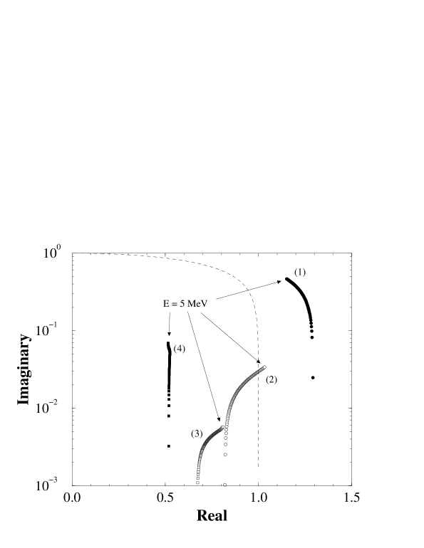
Figure 2: Argand diagrams for the energy variation of the sturmian eigenvalues for $J^{\pi}=1/2^{+}$.

Next, the behavior of $J^{\pi}={3\over 2}^{+}$ eigenvalues are considered. The relevant Argand diagrams are given in Fig. 3. The point values of the largest eigenvalue (labelled (1)) has been i connected by a long-dashed line to guide the eye to link the energy sequence of the results. The actual trajectory is a cusp. That is very evident with curve (1), but similar though more slight features are evident in the trajectories (2) and (3). That cusp feature of the eigenvalue trajectories links to the opening of the $2^{+}_{1}$ state at 4.4389 MeV in the coupled-channel algebra.

Note that these eigenvalues again have small imaginary parts and so the plot is semi-logarithmic and again some details of the trajectories lie below the graphed range. In this case the trajectories do not depart vertically from the real axis at the scattering threshold since they are $d$-wave solutions. The (largest) eigenvalue clearly evolves well beyond the unit after crossing with a quite small imaginary part. Thus it coincides with the lower energy $\frac{3}{2}^{+}$ compound resonance in the cross section. Likewise the 2^nd trajectory crosses the unit circle at higher energy and with a larger imaginary part. This coincides with the known second, broader, $\frac{3}{2}^{+}$ shape resonance at 3.4 MeV. The 3^rd and 4^th sturmian trajectories shown in Fig. 3 track towards the unit circle but have not crossed before 5 MeV.

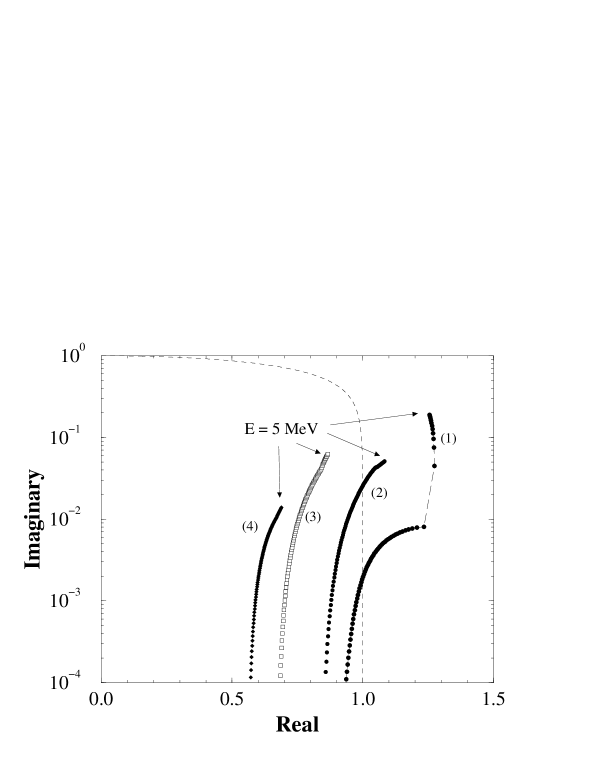
Figure 3: Argand diagram for the energy variation of the sturmian eigenvalues for $J^{\pi}=3/2^{+}$.

Finally, in Fig. 4, we show the Argand diagram of the 2^nd and 3^rd largest eigenvalues for $J^{\pi}={5\over 2}^{+}$ since the first coincides with a state in the mass 13 spectrum below threshold. The unit circle is represented therein by the dashed curve. Again the long-dashed line is simply to guide the eye to the energy variation of these results; results which give rise to a very narrow resonance at E$\simeq$2.086 MeV. As the vertical scale again is logarithmic, the trajectories continue below the graphed limit. The trajectories also exhibit a non-vertical ”take-off’ from the real axis commensurate with them portraying $d$-wave eigenvalues. Also both exhibit cusps which tag to the energy of the $2^{+}_{1}$ state.

Given that the imaginary component of the eigenvalue (curve (2)) is very small, it is a very narrow resonance in the cross section, and the resonance centroid essentially is equivalent to the energy at which the real component of the eigenvalue itself is unity. That resonance in the total cross section is shown in Fig. 5. It has a width of about 15 keV and a magnitude of over 6 barn.

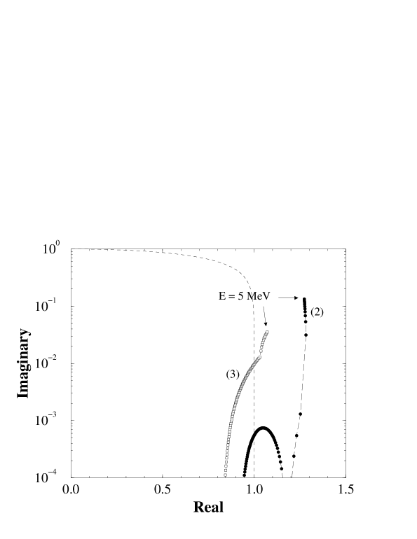
Figure 4: Argand diagram for the energy variation of the sturmian eigenvalues for $J^{\pi}=5/2^{+}$.

Figure 5: The $J^{\pi}=\frac{5}{2}^{+}$ resonance in the elastic scattering cross section.

IV.0.2 Calculation of resonance parameters

To find the resonance centroids and widths, one first has to find all the energies where the real part of the sturmian eigenvalues crosses unity. That determines an approximate value for the resonance energy $E_{R}$ by the condition

$$\zeta_{r}(E_{R})=1+i\delta\,.$$ (47)

Since these eigenvalues change smoothly with energy, it is possible to find these points with a rapidly converging predict-and-correct iterative procedure. We have also estimated the width of these resonances, according to the approximation

$${\Gamma_{R}}\simeq 2\times{dE\over d[{\cal R}(\zeta_{r})]}\delta$$ (48)

where $d[{\cal R}(\zeta_{r})]$ represents the differential of the real part of $\zeta_{r}$ at the resonance energy. These formulas (Eqs. (47) and (48)) are correct in the limit $\delta<<1$, therefore they should be considered reliable only for the narrow resonances. For the case of wider resonances, it is not difficult to find the more complicated expressions required. In the context of the present discussion, however, they are not needed and indeed cross-section evaluations at reasonable energy steps can be used to ascertain them quite easily.

IV.1 The theoretical elastic cross section and polarizations

The method described in the previous subsection enables us to determine with some precision, the centroid energies and widths of all the resonances. Similarly, we can find the energies of the bound states. At the same time we have sought a good theoretical description of the elastic cross section in compare with the data of Fig. 1. The polarizations (at select scattering angles) will follow without having played any part in determining potential parameter values and so are “predictions”.

Starting from the basic potential parameters, we determined all the resonance energies, widths and bound-state energies. That set we denote as $\left\{{E^{(0)}_{i}}\right\}$. Then we changed each parameter by a small amount and calculated a matrix of (approximate) partial derivatives of the $E^{(0)}_{i}$ with respect to the parameters. That matrix of derivatives we denote generically by $\left\{\frac{\partial E^{(0)}_{i}}{\partial\beta_{p}}\right\}$. Then, to first order, a new set of energies $\left\{E_{i}^{(1)}\right\}$ are given by the $n=1$ form of the recursive formula,

$$E_{i}^{(n)}\simeq E^{(n-1)}_{i}+\sum_{p}\frac{\partial E_{i}^{(n-1)}}{\partial\beta_{p}}\Delta\beta_{p}$$ (49)

where $\Delta\beta_{p}$ are the changes in parameters $\beta_{p}$ needed to produce the new $E_{i}^{(n)}$. If the number of parameters is equal to the number of energy values, this set of equations can be considered as a linear system to solve for the $\Delta\beta_{p}$ needed to produce the resultant $E_{i}^{(\rm final)}$. We chose a few of the parameters to vary, and a few essential features of the resonance structure, as given in the data or read off from Fig. 1, in an attempt to produce a fit to that data.

This has turned out to be a rather complex task because of the interplay among the parameters, as well as due to some lack of flexibility of the collective model on which this analysis is based. It can be compared to squeezing a balloon … something always pops out that one wants to keep in. In fact, we carried out this process in two stages. In the first, a quite rough agreement with the data in Fig. 1 was found. This set of parameters was used as a “new base” and the process was repeated. In the end, we obtain a quite good description of the experimental cross section. But some small defects remain, so this result may not be the best that can be achieved. With this multi-dimensional non-linear problem, there may be a number of “quite good” sets of parameters; we have found one.

Rather than attempting to fit everything, we decided to limit ourselves to trying to reproduce the most prominent features of the experimental elastic cross section shown in Fig. 1, and of the experimentally best established resonances. Specifically, we focused on the two ${3\over 2}^{+}$ resonances in the range 2.5 to 4.0 MeV energy, the prominent narrow ${5\over 2}^{+}$ resonance just above 2.0 MeV, and the known bound states below threshold. The collective model used produces two ${3\over 2}^{+}$ resonances in agreement with the data. Of the two, one is very wide ($\Gamma\sim 1$ MeV), likely single-particle, and can account for the broad peak centered around 3.5 MeV. The other is narrow, generally less than 100 keV, and by interference with the first, produces the prominent structure in the cross section near 3.0 MeV. This is shown by the continuous curve in Fig. 6. In this region a narrow ${1\over 2}^{-}$ resonance also is obtained from the model. Such is not seen in the data nor does a partner state exist in the spectrum of ¹³C. Note that in Fig. 6 we use the evaluated cross section data file (ENDF) also found in the website of the National Nuclear Data Center, Brookhaven (www.nndc.bnl.gov).

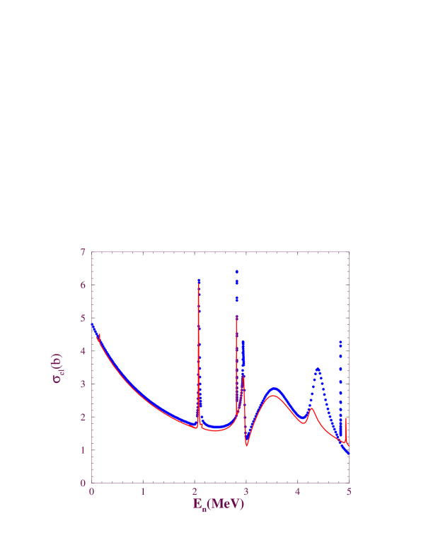
Figure 6: Comparisons between theory (dotted curve) and experimental data (solid curve, ENDF evaluated) of the cross section from the elastic scattering of neutrons from ¹²C.

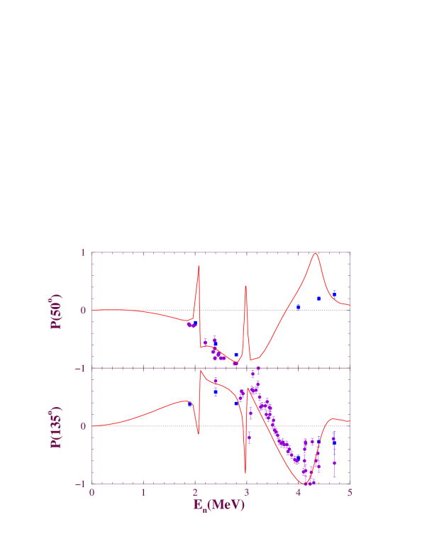
Figure 7: Comparisons between theory (solid curves) and experimental data (filled circles and squares with error bars) of the polarizations from the elastic scattering of neutrons from ¹²C.

Nevertheless, and as can be seen in Fig. 6, the overall agreement between experimental cross-section data and theory is good. The theoretical curve shows the structure just below 3.0 MeV as very similar in shape. The prominent narrow ${5\over 2}^{+}$ is reproduced at the correct energy. The smaller ${7\over 2}^{+}$ is observed in this figure too, and it is near the correct position. At low energy above threshold, the theoretical cross section is in good agreement with the smooth background curve seen in the experimental data. The theoretical curve also displays the bump above 4.0 MeV, though it is higher and broader than the data. This resonance is assessed to have spin-parity of ${1\over 2}^{-}$. A more careful study of the negative-parity resonances at higher energy is required. An appropriate treatment of higher-energy negative-parity states in the collective model should include the $3^{-}$ state at 9.641 MeV in our selected set of channels. By so doing, the dimensionality of the problem increases and computing time with the existing code becomes exorbitant. A new code based on massive parallel architecture is required. Currently such is under construction.

Polarization data (at two scattering angles) are shown in Fig. 7. They are compared with results that come from the $S$ matrices determined by just seeking cross section features. The known resonances and a characteristic change of sign through the broad $\frac{3}{2}^{+}$ resonance centered near 3.5 MeV are well replicated, as is the variation attributable to that centered near 3.0 MeV. We stress that these polarization data were not used in seeking a best set of potential parameters and were the result of but a single calculation (for each scattering angle) using the cross section defined $S$-matrices.

The full set of resonance energies and widths and bound-state energies between -35.0 MeV and +5.0 MeV obtained with these parameters are given in Table 1. It is worth stressing that only when Pauli blocking is treated by including the OPP does the approach give four states of the correct spin-parity and at appropriate energies below the n+¹²C threshold. Results shown in Table 1 for the spectra in the continuum are those obtained using the OPP terms and are also those displayed in Fig. 6.

Table 1: Resonances and bound states found using the resonance identifier equations and the parameter set of Eq. (46).

$J^{\pi}$	Expt. $E_{R}$ Ajzenberg-Selove (1991)	Expt.$\left({1\over 2}\Gamma_{R}\right)$	$E_{R}$	$\left({1\over 2}\Gamma_{R}\right)$	$E_{R}$	$\left({1\over 2}\Gamma_{R}\right)$
	Resonances		with OPP		without OPP
$({1\over 2})^{+}$	4.259 $\pm$ 0.015	0.11	4.833	0.53	–
$({3\over 2})^{+}$	2.9 $\pm$ 0.01 4	0.062	2.965	0.030	2.997	0.025
$({3\over 2})^{+}$	3.472 $\pm$ 0.015	0.5	3.637	0.54	3.642	0.54
$({5\over 2})^{+}$	2.079 $\pm$ 0.003	0.003	2.086	0.015	2.176	0.013
$({5\over 2})^{+}$	–	–	4.370	0.15	4.389	0.16
$({7\over 2})^{+}$	2.77		2.823	8.9 $\times 10^{-7}$	2.823	8.9 $\times 10^{-7}$
$({9\over 2})^{+}$	4.934	0.001	4.836	6.2 $\times 10^{-4}$	4.836	6.2 $\times 10^{-4}$
$({1\over 2})^{-}$	–	–	2.939	5.0 $\times 10^{-3}$	0.0495	1.2 $\times 10^{-3}$
$({3\over 2})^{-}$	–	–	–		2.185	0.049
$({5\over 2})^{-}$	$\simeq+0.1?$		–		2.615	8.4 $\times 10^{-6}$
	Bound states		with OPP		without OPP
$({1\over 2})^{-}$	-4.98		-4.8650		-5.9360
$({1\over 2})^{+}$	-2.0301		-1.9920		-1.8770
$({1\over 2})^{+}$	–		–		-18.9614
$({1\over 2})^{+}$	–		–		-26.5874
$({3\over 2})^{-}$	-1.3671		-1.4640		-0.9433
$({3\over 2})^{-}$	–		–		-3.6152
$({3\over 2})^{-}$	–		–		-10.0836
$({3\over 2})^{+}$	–		–		-21.9417
$({5\over 2})^{-}$	$\simeq+0.1$		-0.0195		-7.9049
$({5\over 2})^{+}$	-1.1833		-1.8720		-1.8178
$({5\over 2})^{+}$	–		–		-22.0019
$({7\over 2})^{-}$	–		–		-6.3119

The last two columns in Table 1 gives the results obtained when Pauli blocking is ignored (by omitting the effects of the OPP). Those results are identified also by the header, “without OPP”. The bound state spectrum that results most clearly shows the spuriosity. Far more states result than are known empirically (for ¹³C), and most are more deeply bound than the known ground state. With the scattering cross sections, that spuriosity is not as well displayed. Indeed by adjusting parameter values we could attain nearly as good a result as found when the OPP is used. However, without the OPP the resonance states are not the correct entries in the coupled-channel sequence. For example, without the OPP, the narrow $\frac{5}{2}$ resonance near 2.0 MeV is the third in sequence rather than the second when Pauli blocking is used. But, the high spin-parity resonances should not be, and are not, affected by Pauli blocking. For example, in both calculated spectra the $\frac{9}{2}$ resonance has the same centroid and width values.

Focusing on the results with the OPP corrections, clearly the essential features of the even-parity resonances are reproduced well. However, this analysis suggests that the experimental resonance at 4.259 MeV would have a $J^{\pi}$ assignment of $5/2^{+}$ and that a broad resonance that does not influence the elastic scattering has a centroid at 4.833 MeV and would have a spin-parity of $1/2^{+}$. Experiment suggests that the $1/2^{+}$ is observed and lies at 4.259 MeV while the $5/2^{+}$ is not to be seen in this energy regime. But it must be remembered that we have limited the process to just three states in ¹²C, and have some allowance in the parameter specifications in the collective model prescription for the interaction potentials. Likewise there are two negative-parity resonant states indicated from these calculations; namely the $1/2^{-}$ “hidden” in the structure above 3.0 MeV and a $5/2^{-}$ which might align with what is a suggestion of a small narrow resonance just above threshold in the data.

Despite the few anomalies, it is clear that this method makes possible exploration of resonance behavior, in this first presentation by using the collective model, and by using purely algebraic means. However, it is also clear that the collective model, coupled with the restrictions imposed by limiting the choice of active target nucleus levels, will never provide as complete agreement with experimental data as one would like. It is planned to define interaction potential matrices from folding a suitable low energy $NN$ force with microscopic model structure such as given by the shell model; a process that has had much success in recent years in analyses of higher energy nucleon-nucleus scattering Amos et al. (2000). Of course Pauli effects would be approximately included via this folding when full antisymmetrization is considered. Therefore, it is of interest at this stage to speculate what might be learned from a more microscopic theory, and that is discussed in the following section.

V The structure of ¹³C in terms of ¹²C plus a neutron

The algebraic scattering program has been applied to low energy neutron scattering from ¹²C. The energy variation of the measured cross section reveals sharp resonances, some of which one may associate with the presence of states in ¹³C. Likewise, the algebraic methods allow prediction of bound states of the n-¹²C system which should correspond to states in ¹³C below threshold. In our first calculation, the structure of $0^{+}_{1}$ (ground), $2^{+}_{1}$ (4.4389 MeV) and $0^{+}_{2}$ (7.65 MeV) states of ¹²C have been taken into account. That such a model should give results characterizing the observed cross section follows from consideration of ($p$-$s$-$d$) shell models for ^12,13C.

The key quantity that relates the structure of the spectrum of ¹³C to the spectrum of ¹²C plus a neutron in a single particle orbit $j$ is the pickup spectroscopic amplitude,

$$S_{\lambda}^{jIJ}=\left\langle{\Psi_{J}^{(\lambda)}(1,2,\cdots,13)}\left\|{{\bf a}_{j}^{\dagger}}\right\|{\Phi_{I}(1,2,\cdots,12)}\right\rangle.$$ (50)

The development applies equally to a proton with the compound system then being ¹³N. The particle coordinates will be omitted hereafter with the identification:

$$|\Psi_{J}^{(\lambda)}\rangle={\rm the\ }\lambda^{\rm th}{\rm state\ of\ }{}^{13}{\rm C\ with\ spin-parity\ }J^{\pi}$$

$$|\Phi_{I}\rangle={\rm the\ state\ in\ }{}^{12}{\rm C\ with\ spin\ }I\ .$$ (51)

Thus, while just three unique spin states in ¹²C are considered, there will be more than 1 state of spin $J^{\pi}$ formed by attaching any specific orbit nucleon. Whether these numbers are predicted by a shell model calculation or instead are extracted from scattering data analysis, there are two sum rules that indicate if the coupling of any single particle state in the spectrum has been exhausted.

The first is the pickup sum rule. It is the result of summing the spectroscopic probabilities over all target (¹²C) states and is

$$\Sigma_{P}=\sum_{I}\left(S_{\lambda}^{jIJ}\right)^{2} = \sum_{I}\left(\left\langle{\Psi_{J}^{(\lambda)}}\left\|{{\bf a}_{j}^{\dagger}}\right\|{\Phi_{I}}\right\rangle\right)^{2}$$ (52)

$$= \sum_{IKm}\left[(-)^{2j}\left\langle IKjm|JM\right\rangle\ \left\langle{\Psi_{J}^{(\lambda)}}\left\|{\bf a}_{j}^{\dagger}\right\|{\Phi_{I}}\right\rangle\right]^{2}\$$

$$= \sum_{IKm}\ (2J+1)^{2}\ \left\langle\Psi_{JM}^{(\lambda)}\left|a_{jm}^{\dagger}\right|\Phi_{IK}\right\rangle\ \left\langle\Phi_{IK}\left|a_{jm}\right|\Psi_{JM}^{(\lambda)}\right\rangle.$$

On closure over the target states, this gives

$$\Sigma_{P}=(2J+1)^{2}\ \sum_{m}\left\langle\Psi_{JM}^{(\lambda)}\left|a_{jm}^{\dagger}a_{jm}\right|\Psi_{JM}^{(\lambda)}\right\rangle=(2J+1)^{2}\ n^{(\lambda)}_{j}\ ,$$ (53)

where $n^{(\lambda)}_{j}$ is the number of nucleons of the appropriate orbit in the particular ¹³C state $|\Psi_{JM}^{(\lambda)}\rangle$. A further summation over all possible values of $j$ gives

$$\sum_{jI}\left(S_{\lambda}^{jIJ}\right)^{2}=(2J+1)^{2}N\ ,$$ (54)

where N is the number of nucleons of the selected type (neutrons in the case considered). For the ¹³C-[¹²C + n] systems, spectroscopic amplitudes have been calculated Rikus and Amos (1980) using a shell model in which the active shells were $0p$-$1s$-$0d$. Recently, the structure of ¹²C has been found Karataglidis et al. (1995) using a complete no-core $(0+2)\hbar\omega$ shell-model. Such has not been used to specify ¹³C as yet. However, the basic details should not be too different to what is discussed. In $S_{(\lambda)}^{jIJ}$ expressing the states of ¹³C in terms of ¹²C plus a neutron are given. They are presented in the order of excitation in ¹³C with the excitation energy shown in column 2. The equivalent energy in the center of mass for n + ¹²C is shown in column 3. The first four entries therefore are closed to neutron scattering from ¹²C. In the incident energy regime to the threshold of excitation of the 2${}^{+}_{1}$, (4.4389 MeV) state in ¹²C, four known resonances are expected coinciding with the spin-parities of the compound system being ${\frac{5}{2}}^{+}|_{(2)};{\frac{3}{2}}^{+}|_{(1)};{\frac{3}{2}}^{+}|_{(2)}$ and ${\frac{1}{2}}^{-}|_{(2)}$. The third of those however is very broad, $\cal O$(MeV), and $R$-matrix studies Rikus and Amos (1980) suggest that it is a single particle potential resonance.

Thus the shell model indicates that the four known states in ¹³C below the n+¹²C threshold are well represented by a neutron coupled to the ground and $2^{+}_{1}$ states of ¹²C and so should be (and are) well defined by the negative energy solutions of the multichannel algebraic scattering problem. Likewise, coupling a neutron to the same states in ¹²C give shell model candidates for states in ¹³C above the n+¹²C threshold; ones that match observations from scattering data. They relate to resonances in the scattering of neutrons from ¹²C which the multichannel scattering theory also defines well. The sizeable components of a neutron coupled to the $2^{+}$ state of ¹²C that the shell model indicates is consistent with the strong coupling we have found necessary via a collective model prescription in these evaluations of scattering observables.

The second sum rule, the stripping sum rule, is formed by completing a sum over all compound mass (¹³C) states. It is important as it indicates whether or not the model calculation may give the large components of any state. That sum rule is defined by

$$\Sigma_{S}=\sum_{J,\lambda}\left(S_{(\lambda)}^{jIJ}\right)^{2} = \sum_{J,M;\lambda m}\left[(-)^{2j}\left\langle JMjm|IK\right\rangle\left\langle\Psi_{J}^{(\lambda)}\left\|\bf a_{j}^{\dagger}\right\|\Phi_{I}\right\rangle\right]^{2}\ ,$$ (55)

$$= \sum_{J,M;\lambda m}(2I+1)^{2}\left\langle\Phi_{IK}\left|a_{jm}\right|\Psi_{JM}^{(\lambda)}\right\rangle\ \left\langle\Psi_{JM}^{(\lambda)}\left|a_{jm}^{\dagger}\right|\Phi_{IK}\right\rangle$$

$$= (2I+1)^{2}\sum_{m}\left\langle\phi_{IK}\left|a_{jm}a_{jm}^{\dagger}\right|\Phi_{IK}\right\rangle\ .$$

Using the (anti)commutation property of the creation/annihilation operators this sum reduces to

$$\Sigma_{S}=(2I+1)^{2}\left[2j+1-n_{j}\right]\ ,$$ (56)

where $n_{j}$ is the number of nucleons in the orbital $j$ in the target (¹²C) state $|\Phi_{IK}\rangle$. In practical calculations one cannot deal with all of the mass 13 levels and so this sum rule is best viewed as an estimate of how much transition strength lies with states other than those investigated.

Using the $p$-$s$-$d$ shell model gives stripping sum rule values listed in Table 3. They are compared against a theoretical limit set assuming that there are no $1s-0d$ neutrons in the ground state description of ¹²C. That is quite reasonable as a shell model study Karataglidis et al. (1995) made using the complete $(0+2)\hbar\omega$ space gives 11.6 nucleons within the $0s-0p$ shells for both the $0^{+}(gs)$ and $2^{+}$(4.4389) states. However, with the simplest of shell models (packed orbits), the pickup sum rule values theoretically are 2, 4, and 6 for the $1s_{1/2},0d_{3/2}$, and $0d_{5/2}$ shells respectively. The occupancies of the $0s_{1/2},0p_{3/2},0p_{1/2}$ used to get the results listed in Table 3 are those given by $p$-$s$-$d$ shell model calculations Rikus and Amos (1980), namely 2.0, 3.288 and 0.712 respectively.

Table 2: Shell model values for pickup spectroscopic amplitudes giving ¹³C for neutrons on ¹²C with energies to 4.0 MeV. Single particle states belong to the $0p-0d-1s$ space.

13C	Eex	E rel. C.M.	neutron	12C	One channel	Two channels
${J}^{\pi}_{(\lambda)}$	in 13C	n + 12C	$\ell_{j}$	${I}$	$S_{(\lambda)}^{j0j}$	$S_{(\lambda)}^{jIJ}$
$\frac{1}{2}^{-}|_{1}$	0.00	-4.95	$p_{1/2}$	0	1.127	1.107
			$p_{3/2}$	2		-1.498
$\frac{1}{2}^{+}|_{1}$	3.09	-1.86	$s_{1/2}$	0	1.349	1.349
			$d_{3/2}$	2		-0.148
			$d_{5/2}$	2		0.069
$\frac{3}{2}^{-}|_{1}$	3.68	-1.26	$p_{3/2}$	0	-0.840	-0.887
			$p_{1/2}$	2		-1.819
			$p_{3/2}$	2		1.122
$\frac{5}{2}^{+}|_{1}$	3.85	-1.09	$d_{5/2}$	0	2.271	2.271
			$s_{1/2}$	2		0.334
			$d_{3/2}$	2		-0.293
			$d_{5/2}$	2		0.415
$\frac{5}{2}^{+}|_{2}$	6.86	1.92	$d_{5/2}$	0	0.409	0.409
			$s_{1/2}$	2		-2.173
			$d_{3/2}$	2		0.234
			$d_{5/2}$	2		0.502
$\frac{7}{2}^{+}|_{1}$	7.49	2.54	$d_{3/2}$	2		0.778
			$d_{5/2}$	2		-2.565
$\frac{5}{2}^{-}|_{1}$	7.55	2.60	$p_{1/2}$	2		1.314
			$p_{3/2}$	2		0.495
$\frac{3}{2}^{+}|_{1}$	7.68	2.73	$d_{3/2}$	0	0.944	0.944
			$s_{1/2}$	2		1.638
			$d_{3/2}$	2		0.192
			$d_{5/2}$	2		0.326
$\frac{3}{2}^{+}|_{2}$	8.20	3.30	$d_{3/2}$	0	-1.000	-1.000
			$s_{1/2}$	2		0.803
			$d_{3/2}$	2		0.318
			$d_{5/2}$	2		-0.644
$\frac{1}{2}^{-}|_{2}$	8.86	3.91	$p_{1/2}$	0	0.082	-0.049
			$p_{3/2}$	2		0.084
$\frac{3}{2}^{-}|_{2}$	9.50	4.55	$p_{3/2}$	0	0.052	-0.075
			$p_{1/2}$	2		-0.102
			$p_{3/2}$	2		1.123
$\frac{3}{2}^{-}|_{3}$	9.90	4.95	$p_{3/2}$	0		0.031
			$p_{1/2}$	2		0.058
			$p_{3/2}$	2		-0.205

For those single particle specifics the theoretical sum rule limits are 0.0, 0.712, and 1.288. In the $2^{+}$ (4.4389 MeV) state in ¹²C, the occupancies are varied slightly from those with the $0p$ shell numbers most altered. The relevant theoretical sum rules then were found using occupancies of 2.0, 3.01, and 0.98. The sum rule exhaustion suggests that the assumption that the states in the listings above are a nucleon plus the ¹²C nucleus in either the ground or the 2⁺ (4.4389 MeV) state is quite well satisfied except if that nucleon is in the $d_{\frac{3}{2}}$ orbit. It would not surprise, therefore, if the excitation of the ¹³C $\frac{3}{2}^{+}$ states may not be as well described as others with any model involving the ground and 2⁺ states of ¹²C in the basis. Note also from Table 2 that the $\frac{7}{2}^{+}$ and $\frac{5}{2}^{-}$ states anticipated to lie at 2.54 and 2.6 MeV excitation in the n-¹²C system, are solely based upon couplings with the ¹²C 2⁺ state. As such they may be only weakly excited in the n-¹²C scattering cross section.

Table 3: The sum rules for the two channel case – neutron space $0p-1s-0d$.

Neutron	12C	Theoretical	Shell model	exhaustion
state	state	sum rule	sum rule	%
$s_{1/2}$	$0^{+}$	2	1.820	91
	$2^{+}$	10	8.387	84
$p_{1/2}$	$0^{+}$	1.240	1.239	100
	$2^{+}$	5.080	5.050	99
$p_{3/2}$	$0^{+}$	0.763	0.758	99
	$2^{+}$	4.935	4.871	99
$d_{3/2}$	$0^{+}$	4	3.110	78
	$2^{+}$	20	0.95	5
$d_{5/2}$	$0^{+}$	6	5.557	93
	$2^{+}$	30	25.281	84

VI conclusions

A model for nucleon-nucleus scattering that uses sturmian expansions of multichannel interactions between the colliding nuclei has been used and found to give resonance scattering upon an average background; typical of what is measured with low-energy experiments. That sturmian expansion theory also gives resonance identifier equations whose solutions identify feasibly, all possible resonance aspects to the scattering problem. Indeed we have found that it is quite practical to find the narrow resonances (compound and quasi-compound) of the coupled-channel Schrödinger problem by diagonalizing the energy-dependent matrix $\mbox{\boldmath$\eta$}^{-{1\over 2}}{\bf G}_{0}(E)\mbox{\boldmath$\eta$}^{-{1\over 2}}$ and studying the trajectories of the relevant eigenvalues in the Gauss plane. When one of these complex eigenvalues evolves past the point $1+i0$ and does so having also a small imaginary component, one of these resonances occurs. Then Eqs. (47) and (refg-res) can be used to determine the resonance parameters. Since these eigenvalues have smooth energy dependencies, it is generally much simpler so to determine the occurrence of resonance states than by other means that have been used to date.

We have used a collective model (to second order) to define a multichannel potential matrix for low-energy neutron-¹²C scattering allowing coupling between the $0^{+}_{1}$ (ground), $2^{+}_{1}$ (4.4389 MeV), and $0^{+}_{2}$ (7.64 MeV) states with coupling taken to second order. The algebraic $S$ matrix for this system has been evaluated. Good results have been found for the sub-threshold bound states and for the cross sections and polarizations as functions of energy. The latter are rich in structure having both narrow and broad resonant features for different $J^{\pi}$; the existence and parameter values of which can be ascertained with ease.

The introduction of the Pauli exclusion principle in the coupled-channel model by means of the orthogonalizing pseudo-potential (OPP) technique ensures that the model gives a spectrum (bound states and resonances) that are built as physical states. This was an important improvement giving an unique identification of states with respect to experimental data.

The results indicate that this approach has predictive power and can be used to interpret the experimental resonance spectra of the nuclear processes at low energy. The discussion on the n-¹²C resonant spectrum contained herein is just one simple example of the potential use of this approach in nuclear analyses.

Appendix A The first generation sturmians

With $l$ being the orbital angular momentum quantum number that is embedded in the set collectively denoted by $c$, the eigenvalues $q_{li}$ of the first generation sturmian problem may be calculated as follows. Consider a square well problem for a binding energy $B$ and well with depth ${\cal V}_{0}$ and radius $R$. With $x_{li}=q_{li}\rho,{\bar{q}}=\sqrt{\mu B}$, and $y={\bar{q}}\rho$, the first eigenvalues are defined from solution of the transcendental equations,

$$x_{li}\cot x_{li}+y=0\ ,$$ (57)

and

$$x_{li}{F_{l-1}(x_{ln})\over F_{l}(x_{li})}+y{\Omega_{l-1}(y)\over\Omega_{l}(y)}=0\ ;\ l>0\ .$$ (58)

The functions $F_{l}$ and $\Omega_{l}$ are the Riccati–Bessel and modified Riccati-Bessel (of the 3^rd kind) functions respectively; each of order $l$. They can be solved using well known recursion formulas Pisent and Canton (1986). In terms of these, the first generation sturmians are

$$\Phi_{li}^{0}(r)=A_{li}\left\{\begin{array}[]{cr}F_{l}(q_{ln}r)&\hskip 14.22636pt{\rm for}\ 0\leq r\leq\rho\\ \left[\frac{F_{l}(q_{li}\rho)}{\Omega_{l}(y)}\right]\Omega_{l}(\bar{q}r)&\hskip 14.22636pt{\rm for}\ r\geq\rho\ .\end{array}\right.$$ (59)

The normalization constant is

$$A_{li}=\sqrt{\frac{\mu}{(q_{li}^{2}+\bar{q}^{2})\int_{0}^{\rho}F_{l}^{2}(q_{li}r)dr}}\ ,$$ (60)

and the sturmian eigenvalue is

$$\eta^{(0)}_{ci}=\frac{\mu{\cal V}_{0}}{q^{2}_{li}+{\bar{q}}^{2}}\ .$$ (61)

Note that the well depth ${\cal V}_{0}$ plays no role in the development of the separable expansions as the product $U_{c}^{0}\left[\eta^{(0)}_{ci}\right]^{-1}$ assures that it does not carry through.

Appendix B The optical potential

Assuming a local form for the elastic channel element of the potential matrix, the optical potential for elastic scattering is defined by

$$V^{opt}(r,r^{\prime};E) = V_{11}(r)+\sum^{C}_{c,c^{\prime}=2}V_{1c}(r)\ G^{(Q)}_{cc^{\prime}}(r,r^{\prime};E)\ V_{c^{\prime}1}(r^{\prime})$$ (62)

$$= V_{11}(r)+\Delta U(r,r^{\prime};E)\ .$$

Here $\Delta U$, the dynamic polarization potential (DPP), makes this formulated interaction complex, nonlocal, and energy dependent as $G^{(Q)}_{cc^{\prime}}$ are the full Green functions referring to the $Q\ (=C-1)$ excluded channels. Those Green functions are solutions of LS type equations built upon the free single channel Green function, $G_{0c}$, namely

$$G^{(Q)}_{cc^{\prime}}=G_{0c}\delta_{cc^{\prime}}+\sum^{C}_{c^{\prime\prime}=2}\ G_{0c}\ V_{cc^{\prime\prime}}\ G^{(Q)}_{c^{\prime\prime}c^{\prime}}\ .$$ (63)

This complex equation is vastly simplified when the interactions are approximated by separable expansions of finite rank and then Canton et al. (1987, 1988); Cattapan et al. (1990)

$$\Delta U(r,r^{\prime};E)=\sum^{N}_{n,n^{\prime}=1}\chi_{1n}(r)\left[{\mbox{\boldmath$\Lambda$}}(E)\right]_{nn^{\prime}}(E)\chi_{n^{\prime}1}(r^{\prime})\ ,$$ (64)

where

$${\mbox{\boldmath$\Lambda$}}(E)=\left[{\mbox{\boldmath$\eta$}}-{\bf G}_{0}^{(Q)}(E)\right]^{-1}-{\mbox{\boldmath$\eta$}}^{-1}$$ (65)

involves

$$\left[{\bf G}_{0}^{(Q)}(E)\right]_{nn^{\prime}}=\mu\left[\sum^{\rm open}_{c\neq 1}\int_{0}^{\infty}\frac{{\hat{\chi}}_{cn}(x){\hat{\chi}}_{cn^{\prime}}(x)}{k_{c}^{2}-x^{2}+i\epsilon}x^{2}dx-\sum^{\rm closed}_{c\neq 1}\int_{0}^{\infty}\frac{{\hat{\chi}}_{cn}(x){\hat{\chi}}_{cn^{\prime}}(x)}{h_{c}^{2}+x^{2}}x^{2}dx\right]\ ,$$ (66)

where $k_{c}$ and $h_{c}$ are respectively the wave numbers relevant for each open and closed channel considered. In application Cattapan et al. (1991); Pisent and Svenne (1995), various perturbative-iterative schemes have been used to evaluate the DPP and thence to determine the (elastic) scattering $S$ matrix.

Appendix C Local potential matrix elements

Using the Woods-Saxon forms

$$f(r)=\left[1+e^{\left({{r-R}\over a}\right)}\right]^{-1}\hskip 8.5359pt;\hskip 8.5359ptg(r)=\frac{1}{r}\frac{df(r)}{dr}\hskip 8.5359pt;\hskip 8.5359ptW_{ls}=2V_{ls}\lambda_{\pi}^{2}\ ,$$ (67)

with $\kappa_{l}=\beta_{L}R_{0}/a$ and the definitions

$$e(r) = \exp{\left(\frac{r-R_{0}}{a}\right)}\hskip 14.22636pt;\hskip 14.22636ptf_{0}(r)=\left[1+e(r)\right]^{-1}$$

$$A(r) = e(r)\ \left[1+e(r)\right]^{-2}=\frac{a}{R_{0}}\left.\frac{df(r)}{d\epsilon}\right|_{0}=-ar\ g_{0}(r)$$

$$B(r) = e(r)\ [e(r)-1]\ \left[1+e(r)\right]^{-3}=\left(\frac{a}{R_{0}}\right)^{2}\left.\frac{d^{2}f(r)}{d\epsilon^{2}}\right|_{0}=-\left({a^{2}r\over R_{0}}\right)\left.{dg\over d\epsilon}\right|_{0}$$

$$C(r) = \frac{e(r)}{\left[1+e(r)\right]^{4}}\left[e^{2}(r)-4e(r)+1\right]=-ar\left({a\over R_{0}}\right)^{2}\left.{d^{2}g\over d\epsilon^{2}}\right|_{0}\ ,$$ (68)

the potential matrix elements, Eq. (37), take the form, omitting the relevant parity indices,

$$V_{c^{\prime}c}(r) = \left\{[V_{0}+l(l+1)\ V_{ll}]\left[f_{0}(r)+1/(8\pi)\ \kappa_{L}^{2}B(r)\right]\right.$$ (69)

$$\hskip 85.35826pt-\frac{1}{ar}\left.W_{ls}\left[A(r)+1/(8\pi)\ \kappa_{L}^{2}C(r)\right][{\bf\ell}{\bf\cdot}{\bf s}]_{c}\right\}\delta_{c^{\prime}c}$$

$$+V_{ss}\left[f_{0}(r)+1/(8\pi)\ \kappa^{2}_{L}B(r)\right]\ [{\bf s}{\bf\cdot}{\bf I}]_{c^{\prime}c}$$

$$+\left\{V_{0}+\frac{1}{2}V_{ll}[l^{\prime}(l^{\prime}+1)+l(l+1)]\right\}\$$

$$\hskip 28.45274pt\times\left\{[4\pi/(2L+1)]^{\frac{1}{2}}\ \kappa_{L}A(r)\ \left[{\bf Y}_{L}{\bf\cdot}{\bf Y}_{L}\right]_{c^{\prime}c}+\frac{1}{2}(2L+1)^{2}\kappa^{2}_{L}B(r)\right.$$

$$\hskip 56.9055pt\left.\times\sum_{\ell=2}\frac{1}{(2\ell+1)}|\langle L0L0|\ell 0\rangle|^{2}\left[{\bf Y}_{\ell}{\bf\cdot}{\bf Y}_{\ell}\right]_{c^{\prime}c}\right\}$$

$$-\frac{1}{2ar}W_{ls}\left\{[{\bf\ell}{\bf\cdot}{\bf s}]_{c^{\prime}}+[{\bf\ell}{\bf\cdot}{\bf s}]_{c}\right\}$$

$$\hskip 28.45274pt\times\left\{[4\pi/(2L+1)]^{\frac{1}{2}}\ \kappa_{L}B(r)\ \left[{\bf Y}_{L}{\bf\cdot}{\bf Y}_{L}\right]_{c^{\prime}c}+\frac{(2L+1)^{2}}{2}\kappa^{2}_{l}C(r)\right.$$

$$\hskip 56.9055pt\left.\times\sum_{\ell=2}\frac{1}{(2\ell+1)}|\langle L0L0|\ell 0\rangle|^{2}\ \left[{\bf Y}_{\ell}{\bf\cdot}{\bf Y}_{\ell}\right]_{c^{\prime}c}\right\}$$

$$+\frac{1}{2}V_{ss}[4\pi/(2L+1)]^{\frac{1}{2}}\ \kappa_{L}A(r)\$$

$$\hskip 28.45274pt\times\sum_{c^{\prime\prime}}\left\{[{\bf s}{\bf\cdot}{\bf I}]_{c^{\prime}c^{\prime\prime}}\ \left[{\bf Y}_{L}{\bf\cdot}{\bf Y}_{L}\right]_{c^{\prime\prime}c}+\ \left[{\bf Y}_{L}{\bf\cdot}{\bf Y}_{L}\right]_{c^{\prime}c^{\prime\prime}}[{\bf s}{\bf\cdot}{\bf I}]_{c^{\prime\prime}c}\right\}$$

$$+\frac{1}{2}V_{ss}\frac{(2L+1)}{2}\kappa^{2}_{L}B(r)\left(\sum_{\ell=2}\frac{1}{(2\ell+1)}|\langle L0L0|\ell 0\rangle|^{2}\ \right.$$

$$\hskip 28.45274pt\times\left.\sum_{c^{\prime\prime}}\left\{[{\bf s}{\bf\cdot}{\bf I}]_{c^{\prime}c^{\prime\prime}}\left[{\bf Y}_{\ell}{\bf\cdot}{\bf Y}_{\ell}\right]_{c^{\prime\prime}c}+\left[{\bf Y}_{\ell}{\bf\cdot}{\bf Y}_{\ell}\right]_{c^{\prime}c^{\prime\prime}}[{\bf s}{\bf\cdot}{\bf I}]_{c^{\prime\prime}c}\right\}\right)\ .$$

For the specific case considered, that of neutron scattering from ¹²C and allowing coupling with the 0⁺ (ground state), the $2^{+}$ (4.4389MeV), and the excited 0⁺ (7.64 MeV) states of ¹²C, the L = 2 multipole only is needed in the deformation expansions. Using the specific values for the parity Clebsch-Gordan coefficients of

$$\langle 2020|00\rangle=\frac{1}{\sqrt{5}}\ \ ;\ \ \langle 2020|20\rangle=-\sqrt{\frac{2}{7}}\ \ ;\ \ \langle 2020|40\rangle=3\sqrt{\frac{2}{35}}$$ (70)

gives the result

$$V_{c^{\prime}c}(r) = \left\{[V_{0}+l(l+1)\ V_{ll}]\left[f_{0}(r)+1/(8\pi)\ \kappa_{2}^{2}B(r)\right]\right.$$ (71)

$$\hskip 85.35826pt-\frac{1}{ar}\left.W_{ls}\left[A(r)+1/(8\pi)\ \kappa_{2}^{2}C(r)\right][{\bf\ell}{\bf\cdot}{\bf s}]_{c}\right\}\delta_{c^{\prime}c}$$

$$+V_{ss}\left[f_{0}(r)+1/(8\pi)\ \kappa^{2}_{2}B(r)\right]\ [{\bf s}{\bf\cdot}{\bf I}]_{c^{\prime}c}$$

$$+\left\{V_{0}+\frac{1}{2}V_{ll}[l^{\prime}(l^{\prime}+1)+l(l+1)]\right\}\$$

$$\hskip 14.22636pt\times\left\{\left(\sqrt{(4\pi/5)}\kappa_{2}A(r)+\frac{\kappa_{2}^{2}}{7}B(r)\right)\left[{\bf Y}_{2}{\bf\cdot}{\bf Y}_{2}\right]_{c^{\prime}c}+\frac{\kappa_{2}^{2}}{7}B(r)\left[{\bf Y}_{4}{\bf\cdot}{\bf Y}_{4}\right]_{c^{\prime}c}\right\}$$

$$-\frac{1}{2ar}W_{ls}\left\{[{\bf\ell}{\bf\cdot}{\bf s}]_{c^{\prime}}+[{\bf\ell}{\bf\cdot}{\bf s}]_{c}\right\}$$

$$\hskip 14.22636pt\times\left\{\left(\sqrt{(4\pi/5)}\kappa_{2}B(r)+\frac{\kappa_{2}^{2}}{7}C(r)\right)\left[{\bf Y}_{2}{\bf\cdot}{\bf Y}_{2}\right]_{c^{\prime}c}+\frac{\kappa_{2}^{2}}{7}C(r)\left[{\bf Y}_{4}{\bf\cdot}{\bf Y}_{4}\right]_{c^{\prime}c}\right\}$$

$$+\frac{1}{2}V_{ss}\left\{\left(\sqrt{(4\pi/5)}\kappa_{2}A(r)+\frac{\kappa_{2}^{2}}{7}B(r)\right)\right.$$

$$\hskip 14.22636pt\times\sum_{c^{\prime\prime}}\left[[{\bf s}{\bf\cdot}{\bf I}]_{c^{\prime}c^{\prime\prime}}\ \left[{\bf Y}_{2}{\bf\cdot}{\bf Y}_{2}\right]_{c^{\prime\prime}c}+\ \left[{\bf Y}_{2}{\bf\cdot}{\bf Y}_{2}\right]_{c^{\prime}c^{\prime\prime}}[{\bf s}{\bf\cdot}{\bf I}]_{c^{\prime\prime}c}\right]$$

$$\hskip 28.45274pt\left.+\frac{\kappa_{2}^{2}}{7}B(r)\sum_{c^{\prime\prime}}\left[[{\bf s}{\bf\cdot}{\bf I}]_{c^{\prime}c^{\prime\prime}}\ \left[{\bf Y}_{4}{\bf\cdot}{\bf Y}_{4}\right]_{c^{\prime\prime}c}+\ \left[{\bf Y}_{4}{\bf\cdot}{\bf Y}_{4}\right]_{c^{\prime}c^{\prime\prime}}[{\bf s}{\bf\cdot}{\bf I}]_{c^{\prime\prime}c}\right]\right\}\,.$$

In deriving Eq. (71) from Eq. (37), use has been made of the matrix elements:

$$\langle\mbox{\boldmath$\ell\cdot\ell$}\rangle=\langle\ell^{\prime}j^{\prime}I^{\prime}J|\mbox{\boldmath$\ell\cdot\ell$}|\ell jIJ\rangle=\delta_{\ell\ell^{\prime}}\delta_{jj^{\prime}}\delta_{II^{\prime}}\ell(\ell+1)\ ,$$ (72)

and

$$\langle\mbox{\boldmath$s\cdot\ell$}\rangle=\delta_{\ell\ell^{\prime}}\delta_{jj^{\prime}}\delta_{II^{\prime}}\times\left\{\begin{array}[]{ccc}\frac{\ell}{2}&{\rm,if}&j=\ell+\frac{1}{2}\\ -\frac{\ell+1}{2}&{\rm,if}&j=\ell-\frac{1}{2}\\ \end{array}\right..$$ (73)

The spin-spin matrix element is a little more complicated Varshalovich et al. (1988), namely:

$$\langle{\bf s}{\bf\cdot}{\bf I}\rangle = (-)^{(j+j^{\prime}+J)}\left\{\begin{array}[]{ccc}j^{\prime}&j&1\\ I&I^{\prime}&J\\ \end{array}\right\}\left\langle I^{\prime}\left\|{\bf I}\right\|I\right\rangle\left\langle s\left\|{\bf s}\right\|s\right\rangle$$ (81)

$$= \delta_{II^{\prime}}\delta_{ll^{\prime}}(-)^{\left(1/2+j-j^{\prime}+I+J+l\right)}\sqrt{(2j+1)(2j^{\prime}+1)(2I+1)}$$

$$\hskip 28.45274pt\times\sqrt{\frac{3}{2}I(I+1)}\left\{\begin{array}[]{ccc}j^{\prime}&j&1\\ I&I&J\\ \end{array}\right\}\left\{\begin{array}[]{ccc}\frac{1}{2}&l&j\\ j^{\prime}&1&\frac{1}{2}\\ \end{array}\right\}\ .$$

Since the operator is diagonal in I and $\ell$, and null if either I or I’ is null, for our calculations the following particular case is useful:

$$\langle\ell j^{\prime}2J|{\bf s}{\bf\cdot}{\bf I}|\ell j2J\rangle=\frac{1}{2(2\ell+1)}K(\ell,j,j^{\prime},J).$$ (82)

The values of interest for $K$ are the following:

$$K(\ell,\ell+\frac{1}{2},\ell+\frac{1}{2},J) = -\ell(\ell+2)+J(J+1)-\frac{27}{4},$$ (83)

$$K(\ell,\ell-\frac{1}{2},\ell-\frac{1}{2},J) = \ell^{2}-J(J+1)+\frac{23}{4},$$ (84)

$$K(\ell,\ell+\frac{1}{2},\ell-\frac{1}{2},J) = K(\ell,\ell-\frac{1}{2},\ell+\frac{1}{2},J)$$

$$= \sqrt{(J+\ell+\frac{7}{2})(J+\ell-\frac{3}{2})(J-\ell+\frac{5}{2})(-J+\ell+\frac{5}{2})}\ .$$

We give, finally, the matrix elements of the scalar product of two rank L spherical harmonics as

$$\langle{\bf Y}_{L}{\bf\cdot}{\bf Y}_{L}\rangle = \left\langle{l^{\prime}j^{\prime}I^{\prime}J}\left|{\bf Y}_{L}(\hat{r}){\bf\cdot}{\bf Y}_{L}(\hat{\Upsilon})\right|ljIJ\right\rangle$$ (93)

$$= (-)^{\left(j+I^{\prime}+J\right)}\left\{\begin{array}[]{ccc}j^{\prime}&j&L\\ I&I^{\prime}&J\\ \end{array}\right\}\left\langle\left(l^{\prime}{\frac{1}{2}}\right)j^{\prime}\right\|{\bf Y}_{L}(\hat{r})\left\|\left(l{\frac{1}{2}}\right)j\right\rangle\left\langle I^{\prime}\left\|{\bf Y}_{L}(\hat{\Upsilon})\right\|I\right\rangle$$

$$= (-)^{\left(j+I^{\prime}+l^{\prime}-{\frac{1}{2}}\right)}\sqrt{(2j+1)(2j^{\prime}+1)(2I+1)(2l+1)}\frac{1}{4\pi}(2L+1)$$

$$\hskip 14.22636pt\times\left\langle I0L0|I^{\prime}0\right\rangle\left\langle l0L0|l^{\prime}0\right\rangle\left\{\begin{array}[]{ccc}j^{\prime}&j&L\\ I&I&J\\ \end{array}\right\}\left\{\begin{array}[]{ccc}l&\frac{1}{2}&j\\ j^{\prime}&L&l^{\prime}\\ \end{array}\right\}\ ,$$

then, on using the identity

$$\left\{\begin{array}[]{ccc}l&\frac{1}{2}&j\\ j^{\prime}&L&l^{\prime}\\ \end{array}\right\}\left\langle l0L0|l^{\prime}0\right\rangle=(-)^{\left(l+j^{\prime}+\frac{1}{2}\right)}\frac{1}{\sqrt{(2l+1)(2j^{\prime}+1)}}\left\langle j{\frac{1}{2}}L0\right|\left.j^{\prime}{\frac{1}{2}}\right\rangle\ ,$$ (94)

Eq. (93) reduces to

$$\left\langle l^{\prime}j^{\prime}I^{\prime}J\left|{\bf Y}_{L}({\hat{r}}){\bf\cdot}{\bf Y}_{L}({\hat{\Upsilon}})\right|ljIJ\right\rangle = (-)^{\left(J-{\frac{1}{2}}\right)}\frac{1}{4\pi}\sqrt{(2I+1)(2j+1)(2j^{\prime}+1)(2L+1)}$$ (97)

$$\times\left\langle I0L0|I^{\prime}0\right\rangle\left\langle j{\frac{1}{2}}j^{\prime}{-\frac{1}{2}}\left|\right.L0\right\rangle\left\{\begin{array}[]{ccc}j^{\prime}&j&L\\ I&I^{\prime}&J\\ \end{array}\right\}\ .$$

References

- Lane and Robson (1966) A. M. Lane and D. Robson, Phys. Rev. 151, 774 (1966), and references cited therein.
- Rikus and Amos (1980) L. Rikus and K. Amos, J. Phys. G6, 1535 (1980).
- Pisent and Canton (1986) G. Pisent and L. Canton, Nuovo Cim. A91, 33 (1986).
- Canton et al. (1987) L. Canton, G. Cattapan, and G. Pisent, Nuovo Cim. A97, 319 (1987).
- Canton et al. (1988) L. Canton, G. Cattapan, and G. Pisent, Nucl. Phys. A487, 333 (1988).
- Cattapan et al. (1990) G. Cattapan, L. Canton, and G. Pisent, Phys. Lett. B240, 1 (1990), and references cited therein.
- Cattapan et al. (1991) G. Cattapan, L. Canton, and G. Pisent, Phys. Rev. C 43, 1395 (1991), and references cited therein.
- Pisent and Svenne (1995) G. Pisent and J. P. Svenne, Phys. Rev. C 51, 3211 (1995).
- Rawitscher (1982) G. H. Rawitscher, Phys. Rev. C 25, 2196 (1982).
- Rawitscher and Delic (1984) G. H. Rawitscher and G. Delic, Phys. Rev. C 29, 1153 (1984).
- Tamura (1965) T. Tamura, Rev. Mod. Phys. 37, 679 (1965).
- Ajzenberg-Selove (1991) F. Ajzenberg-Selove, Nucl. Phys. A523, 1 (1991).
- Canton et al. (1991) L. Canton, Y. Hahn, and G. Cattapan, Phys. Rev. C 43, 2441 (1991).
- Weinberg (1965) S. Weinberg, in Lectures on Particles and Field Theory (Prentice-Hall, Englewood Cliffs, N. J., 1965), vol. Brandeis Summer Institute in Theoretical Physics vol 2., p. 289.
- Rawitscher and Canton (1991) G. H. Rawitscher and L. Canton, Phys. Rev. C 44, 60 (1991).
- Pisent and Saruis (1967) G. Pisent and A. M. Saruis, Nucl. Phys. 91, 561 (1967).
- Pascolini et al. (1969) A. Pascolini, G. Pisent, and F. Zardi, Lett. Nuovo Cim. 1, 643 (1969).
- Mikoshiba et al. (1971) O. Mikoshiba, T. Terasawa, and M. Tanifugi, Nucl. Phys. A168, 417 (1971).
- Varshalovich et al. (1988) D. A. Varshalovich, A. N. Moskalev, and V. K. Kersonskii, Quantum Theory of Angular Momentum (World Scientific, Singapore, 1988).
- Mahaux and Weidenmuller (1969) C. Mahaux and H. A. Weidenmuller, Shell-model approach to nuclear reactions (North-Holland, Amsterdam, 1969).
- Kukulin and Pomerantsev (1978) V. Kukulin and V. Pomerantsev, Ann. of Phys. 111, 330 (1978).
- Krasnopol’sky and Kukulin (1974) V. Krasnopol’sky and V. Kukulin, Soviet J. Nucl. Phys. 20, 883 (1974).
- Saito (1969) S. Saito, Prog. Theor. Phys. 41, 705 (1969).
- Hodgson (1971) P. E. Hodgson, Nuclear Reactions and Nuclear Structure (Clarendon Press, Oxford, 1971).
- Amos et al. (2000) K. Amos, P. J. Dortmans, H. V. von Geramb, S. Karataglidis, and J. Raynal, Adv. in Nucl. Phys. 25, 275 (2000).
- Karataglidis et al. (1995) S. Karataglidis, P. J. Dortmans, K. Amos, and R. de Swiniarski, Phys. Rev. C 52, 861 (1995).