Regarding proton form factors

Abstract

The proton’s elastic electromagnetic form factors are calculated using an Ansatz for the nucleon’s Poincaré covariant Faddeev amplitude that only retains scalar diquark correlations. A spectator approximation is employed for the current. On the domain of $q^{2}$ accessible in modern precision experiments these form factors are a sensitive probe of nonperturbative strong interaction dynamics. The ratio of Pauli and Dirac form factors can provide realistic constraints on models of the nucleon and thereby assist in developing an understanding of nucleon structure.

1 Introduction

The pion’s elastic electromagnetic form factor is accessible via a properly constructed six-point quark Schwinger function, a fact exploited with modest success in lattice-QCD simulations, e.g., Refs. [1, 2, 3]. This Schwinger function is also the basis for continuum studies, among which those employing the Dyson-Schwinger equations (DSEs) [4, 5, 6] are efficacious [7]. The proton’s form factors are accessible through an analogous eight-point quark Schwinger function, which is the starting point for lattice simulations, e.g. Refs. [8, 9]. The fruitful extension of DSE methods to the calculation of this Schwinger function is a contemporary goal. As we will explain, a simple truncation that corresponds to a spectator approximation is currently in widespread use [10, 11, 12]. Manifest covariance is a strength of this approach for it has long been apparent that in order to obtain an internally consistent understanding of proton form factor data at spacelike momentum transfers $q^{2}\gtrsim M^{2}$, where $M$ is the proton’s mass, a Poincaré covariant description of the scattering process is necessary [13, 14]. This has recently been reemphasised in the context of constituent-quark models [15, 16, 17].

The same interaction which describes the structure and properties of colour-singlet mesons also generates a quark-quark (diquark) correlation in the colour antitriplet ($\bar{3}$) channel [18, 19]. Such correlations have recently been observed in simulations of lattice-QCD [20]. While diquarks do not survive as asymptotic states [21, 22, 23]; viz., they do not appear in the strong interaction spectrum, the existence of strong quark-quark correlations provides a foundation for viewing the nucleon as a quark-diquark composite. This picture can be realised via a Poincaré covariant Faddeev equation [24], in which two quarks are always correlated as a $\bar{3}$-diquark, and binding in the nucleon is effected by the iterated exchange of roles between the dormant and diquark-participant quarks, and through the action of a pion “cloud” [25].

Upon solving the Faddeev equation one obtains the nucleon’s mass, and also its Faddeev amplitude which is a valuable intuitive tool. It is noteworthy that even a rudimentary covariant Faddeev equation model, based on the presence of diquark correlations within the nucleon, yields a matrix-valued amplitude that, in the nucleon’s rest frame, corresponds to a relativistic wave function with a material lower component; i.e., a wave function with “$p$-wave,” and, indeed, “$d$-wave” correlations, too [26]. Nonzero quark orbital angular momentum in the nucleon is a straightforward outcome of a Poincaré covariant description.

While some issues remain unresolved [27, 28], contemporary data [29, 30, 31] suggest that a single dipole mass cannot simultaneously characterise the $Q^{2}$-dependence of both the proton’s electric and magnetic form factors. This possibility was evident in the Faddeev-amplitude-based calculations of Ref. [10], as emphasised in Ref. [11]. Moreover, it can be inferred from Ref. [32] that this experimental result is an essential consequence of a nonperturbative and Poincaré covariant representation of the proton as a bound state. This may be exemplified through the role played by pseudovector components of the pion’s Bethe-Salpeter amplitude, which are connected with the presence of quark orbital angular momentum in the pion. These pseudovector amplitudes are necessarily nonzero [33] and responsible for the large-$Q^{2}$ behaviour of the electromagnetic pion form factor [34, 35].

Herein we calculate the proton’s elastic electromagnetic form factors, using a product Ansatz for the proton’s Faddeev amplitude and a spectator approximation to describe elastic electromagnetic scattering from the nucleon. We describe the model in Sect. 2, and present and discuss the results in Sect. 3. Section 4 is an epilogue. The study furnishes a means by which we may explore and illustrate the points outlined above. It will become apparent that existing precision data on the form factor ratios $F_{2}^{p}(q^{2})/F_{1}^{p}(q^{2})$ and $G_{E}^{p}(q^{2})/G_{M}^{p}(q^{2})$ are a sensitive probe of nonperturbative aspects of the proton’s structure.

2 Model Elements

2.1 Dressed quarks

There are three primary elements of our model and to begin with its specification we note that quarks within bound states are described by a dressed propagator

$$S(p)=-i\gamma\cdot p\,\sigma_{V}(p^{2})+\sigma_{S}(p^{2})\;=\;\frac{1}{i\gamma\cdot p\,A(p^{2})+B(p^{2})}\;=\;\frac{Z(p^{2})}{i\gamma\cdot p+M(p^{2})}\,.$$ (1)

It is a longstanding, model-independent DSE prediction that the wave function renormalisation $Z(p^{2})$ and mass function $M(p^{2})$ exhibit significant momentum dependence for $p^{2}\lesssim 2\,$GeV² whose origin is nonperturbative [4, 5, 6]. This behaviour was recently verified in numerical simulations of quenched QCD [36], and the connection between this and the full theory is analysed in Ref. [37].

The mass function is enhanced at infrared momenta, a feature that is an essential consequence of the dynamical chiral symmetry breaking (DCSB) mechanism. It is also the origin of the constituent-quark mass. With increasing spacelike $p^{2}$, on the other hand, the mass function evolves to reproduce the asymptotic behaviour familiar from perturbative analyses and that behaviour is manifest for $p^{2}\gtrsim 10\,$GeV² [38].

While numerical solutions for the dressed-quark propagator are readily obtained from a model of QCD’s gap equation, the utility of an algebraic form for $S(p)$ when calculations require the evaluation of numerous multidimensional integrals is self-evident. An efficacious parametrisation, which exhibits the features described above and has been used extensively [4, 5, 6], is expressed via

$$\bar{\sigma}_{S}(x) = 2\,\bar{m}\,{\cal F}(2(x+\bar{m}^{2}))+{\cal F}(b_{1}x)\,{\cal F}(b_{3}x)\,\left[b_{0}+b_{2}{\cal F}(\epsilon x)\right]\,,$$ (2)

$$\bar{\sigma}_{V}(x) = \frac{1}{x+\bar{m}^{2}}\,\left[1-{\cal F}(2(x+\bar{m}^{2}))\right]\,,$$ (3)

with $x=p^{2}/\lambda^{2}$, $\bar{m}$ = $m/\lambda$,

$${\cal F}(x)=\frac{1-\mbox{\rm e}^{-x}}{x}\,,$$ (4)

$\bar{\sigma}_{S}(x)=\lambda\,\sigma_{S}(p^{2})$ and $\bar{\sigma}_{V}(x)=\lambda^{2}\,\sigma_{V}(p^{2})$. The mass-scale, $\lambda=0.566\,$GeV, and parameter values

$$\begin{array}[]{ccccc}\bar{m}&b_{0}&b_{1}&b_{2}&b_{3}\\ \hline\cr 0.00897&0.131&2.90&0.603&0.185\end{array}\;,$$ (5)

were fixed in a least-squares fit to light-meson observables [39]. The dimensionless $u=d$ current-quark mass in Eq. (5) corresponds to

$$m=5.1\,{\rm MeV}\,.$$ (6)

The parametrisation yields a Euclidean constituent-quark mass

$$M_{u,d}^{E}=0.33\,{\rm GeV},$$ (7)

defined as the solution of $p^{2}=M^{2}(p^{2})$ [38], whose magnitude is typical of that employed in constituent-quark models [40]. This is an expression of DCSB, as is the vacuum quark condensate

$$-\langle\bar{q}q\rangle_{0}^{1\,{\rm GeV}^{2}}=\lambda^{3}\,\frac{3}{4\pi^{2}}\,\frac{b_{0}}{b_{1}\,b_{3}}\,\ln\frac{1\,{\rm GeV}^{2}}{\Lambda_{\rm QCD}^{2}}=(0.221\,{\rm GeV})^{3}\,,$$ (8)

$\Lambda_{\rm QCD}=0.2\,$GeV. The condensate is calculated directly from its gauge invariant definition [33] after making allowance for the fact that Eqs. (2), (3) yield a chiral-limit quark mass function with anomalous dimension $\gamma_{m}=1$. This omission of the additional $\ln(p^{2}/\Lambda_{\rm QCD}^{2})$-suppression that is characteristic of QCD is merely a practical simplification.

2.2 Product Ansatz for the Faddeev amplitude

We represent the proton as a composite of a dressed-quark and nonpointlike, Lorentz-scalar quark-quark correlation (diquark), and exhibit this via a product Ansatz for the Faddeev amplitude

$$\Psi_{3}^{0^{+}}(p_{i},\alpha_{i},\tau_{i}) = [\Gamma^{0^{+}}(\frac{1}{2}p_{[12]};K)]_{\alpha_{1}\alpha_{2}}^{\tau_{1}\tau_{2}}\,\Delta^{0^{+}}(K)\,[{\cal S}(\ell;P)u(P)]_{\alpha_{3}}^{\tau_{3}}\,,$$ (9)

wherein $(p_{i},\alpha_{i},\tau_{i})$ are the momentum, spin and isospin labels of the quarks constituting the nucleon; the spinor satisfies

$$\bar{u}(P)\,(i\gamma\cdot P+M)=0=(i\gamma\cdot P+M)\,u(P)\,,$$ (10)

with $P=p_{1}+p_{2}+p_{3}$ the nucleon’s total momentum, and it is also a spinor in isospin space with $\varphi_{+}={\rm col}(1,0)$ for the proton and $\varphi_{-}={\rm col}(0,1)$ for the neutron; and $K=p_{1}+p_{2}=:p_{\{12\}}$, $p_{[12]}=p_{1}-p_{2}$, $\ell:=(-p_{\{12\}}+2p_{3})/3$.

In Eq. (9), $\Delta^{0^{+}}(K)$ is a pseudoparticle propagator for the scalar diquark formed from quarks $1$ and $2$, and $\Gamma^{0^{+}}\!$ is a Bethe-Salpeter-like amplitude describing their relative momentum correlation. These functions can be obtained from an analysis of the quark-quark scattering matrix, as explained in Ref. [25]. However, we have already chosen to simplify our calculations by parametrising $S(p)$, and hence we follow Refs. [10, 11] and also employ that expedient herein, using

$$\Delta^{0^{+}}(K) = \frac{1}{m_{0^{+}}^{2}}\,{\cal F}(K^{2}/\omega_{0^{+}}^{2})\,,$$ (11)

$$\Gamma^{0^{+}}(k;K) = \frac{1}{{\cal N}^{0^{+}}}\,H\,Ci\gamma_{5}\,i\tau_{2}\,{\cal F}(k^{2}/\omega_{0^{+}}^{2})\,,$$ (12)

with ${\cal F}$ defined in Eq. (4), $C=\gamma_{2}\gamma_{4}$ the charge conjugation matrix, $\tau_{2}$ the $2\times 2$ Pauli isospin matrix, and $(H^{c_{3}})_{c_{1}c_{2}}=\epsilon_{c_{1}c_{2}c_{3}}$, $c_{1,2,3}=1,2,3$, describing the completely antisymmetric colour structure of a $\bar{3}$ diquark. The parameters are a width, $\omega_{0^{+}}$, and a pseudoparticle mass, $m_{0^{+}}$, which have ready physical interpretations: the length $l_{0^{+}}=1/\omega_{0^{+}}$ is a measure of the mean separation between the quarks in the scalar diquark; and the distance $\lambda_{0^{+}}=1/m_{0^{+}}$ represents the range over which a diquark correlation in this channel can persist inside the nucleon.

With the elements described hitherto it is possible to derive a Poincaré covariant Faddeev equation whose solution yields ${\cal S}$, a $4\times 4$ Dirac matrix that describes the relative quark-diquark momentum correlation. The complete nucleon amplitude then follows:

$$\Psi=\Psi_{1}+\Psi_{2}+\Psi_{3}\,,$$ (13)

where the subscript identifies the dormant quark and, e.g., $\Psi_{1,2}$ are obtained from $\Psi_{3}$ by a uniform, cyclic permutation of all the quark labels. The general form of ${\cal S}$ is discussed at length in Ref. [26] with the conclusion that the positive energy solution can be written

$${\cal S}(\ell;P)=f_{1}(\ell;P)\,I_{\rm D}+\frac{1}{M}\left(i\gamma\cdot\ell-\ell\cdot\hat{P}\,I_{\rm D}\right)\,f_{2}(\ell;P)\,,$$ (14)

where $(I_{\rm D})_{rs}=\delta_{rs}$, $\hat{P}^{2}=-1$. In the nucleon’s rest frame, $f_{1,2}$, respectively, describe the upper, lower component of the spinor amplitude ${\cal S}(\ell;P)\,u(P)$.

Again, calculations are simplified if one employs an algebraic parametrisation of ${\cal S}$, and the form [41]

$${\cal S}(\ell;P)=\frac{1}{{\cal N}_{\Psi}}\,{\cal F}(\ell^{2}/\omega^{2}_{q\{qq\}})\,\left[I_{\rm D}-\frac{\mbox{\sc r}}{M}\left(i\gamma\cdot\ell-\ell\cdot\hat{P}\,I_{\rm D}\right)\right]$$ (15)

is efficacious. In writing this one exploits results of the Faddeev equation calculations reported in Refs. [25, 26], which establish the fidelity of the approximations $f_{2}(\ell;P)\approx\mbox{\sc r}f_{1}(\ell;P)$ and $f_{1}(\ell;P)\approx f_{1}(\ell^{2};P^{2})$. The Ansatz involves two parameters: a width $\omega_{q\{qq\}}$ and ratio r. The former can be associated with a length-scale $l_{q\{qq\}}=1/\omega_{q\{qq\}}$, which measures the quark-diquark separation. The latter gauges the importance of the lower component of the positive energy nucleon’s spinor amplitude. Its magnitude increases with increasing r. (The strength of the lower component of the nucleon’s Faddeev wave function is determined by r but does not vanish for $\mbox{\sc r}=0$.) In realistic Faddeev equation studies of the nucleon $l_{q\{qq\}}>l_{0^{+}}/2\sim 0.2\,$fm and $\mbox{\sc r}\sim 0.5$ [25].

2.3 Dressed-quark-photon coupling

A calculation of the electromagnetic interaction of a composite particle cannot proceed without an understanding of the coupling between the photon and the bound state’s constituents. If those constituents are dressed then the coupling is not pointlike. Indeed, it is readily apparent that with quarks dressed as described in Sec. 2.1, only a dressed-quark-photon vertex, $\Gamma_{\mu}$, can satisfy the vector Ward-Takahashi identity:

$$q_{\mu}\,i\Gamma_{\mu}(\ell_{1},\ell_{2})=S^{-1}(\ell_{1})-S^{-1}(\ell_{2})\,,$$ (16)

where $q=\ell_{1}-\ell_{2}$ is the photon momentum flowing into the vertex. This is illustrated with particular emphasis in Refs. [35, 42, 43, 44, 45, 46, 47], which consider effects associated with the Abelian anomaly. The Ward-Takahashi identity is only one of many constraints that apply to $\Gamma_{\mu}$ in a renormalisable quantum field theory and these have been explored extensively in Refs. [48, 49].

The dressed-quark-photon vertex, a three-point Schwinger function, can be obtained by solving an inhomogeneous Bethe-Salpeter equation. This was the procedure adopted in the DSE calculation [7] that successfully predicted the electromagnetic pion form factor [50]. For our purposes, however, it is enough to follow Ref. [39] and employ the algebraic parametrisation [51]

$$i\Gamma_{\mu}(\ell_{1},\ell_{2})=i\Sigma_{A}(\ell_{1}^{2},\ell_{2}^{2})\,\gamma_{\mu}+(\ell_{1}+\ell_{2})_{\mu}\left[\mbox{\footnotesize$\displaystyle\frac{1}{2}$}i\gamma\cdot(\ell_{1}+\ell_{2})\,\Delta_{A}(\ell_{1}^{2},\ell_{2}^{2})+\Delta_{B}(\ell_{1}^{2},\ell_{2}^{2})\right];$$ (17)

with

$$\Sigma_{F}(\ell_{1}^{2},\ell_{2}^{2})=\mbox{\footnotesize$\displaystyle\frac{1}{2}$}\,[F(\ell_{1}^{2})+F(\ell_{2}^{2})]\,,\;\Delta_{F}(\ell_{1}^{2},\ell_{2}^{2})=\frac{F(\ell_{1}^{2})-F(\ell_{2}^{2})}{\ell_{1}^{2}-\ell_{2}^{2}}\,,$$ (18)

where $F=A,B$; i.e., the scalar functions in Eq. (1). It is critical that $\Gamma_{\mu}$ in Eq. (17) satisfies Eq. (16) and very useful that it is completely determined by the dressed-quark propagator. Improvements to this Ansatz modify results by $\lesssim 10\,$%, as illustrated, e.g., in Refs. [52, 53].

Equation (17) entails that dressed-quarks do not respond as point particles to low momentum transfer probes. This observation qualitatively supports an assumption employed in some relativistic constituent quark models [13, 15, 54]. An unambiguous quantitative connection is difficult because the definition of constituent-quark degrees of freedom depends on a model’s formulation. It may nevertheless be worth noting that quark dressing disappears with increasing spacelike $q^{2}$ in QCD. Hence, in the ultraviolet, the dressed-quark’s Dirac form factor must approach one (with only $\ln q^{2}$ corrections) and its Pauli form factor must vanish; viz., the interaction becomes pointlike in this limit. With the parameter values in Eq. (5), this evolution of the Dirac and Pauli form factors may be characterised by monopole ranges $r_{1}\sim 0.25\,$fm and $r_{2}\sim 0.35\,$fm, respectively.

2.4 Commentary

We have completely specified a covariant model of the nucleon as a bound state of a dressed-quark and nonpointlike scalar quark-quark correlation. This algebraic Ansatz has four parameters: $m_{0^{+}}$ and $\omega_{0^{+}}$ introduced in Eqs. (11), (12) to characterise the diquark; and $\omega_{q\{qq\}}$ and r in Eq. (15), which express prominent features of the nucleon’s spinor. The dressed-quark propagator and dressed-quark-photon vertex are fixed.

In contemplating such a model one may ask whether it can supply an accurate description of the nucleon’s electromagnetic form factors. A priori, the answer is unknown but it is supplied by straightforward calculations.

A more important question, however, is whether the model should be accurate. In this case the answer is no. Reference [25] emphasises that no picture of the nucleon is veracious if it neglects axial-vector diquark correlations and the nucleon’s pion “cloud.” Thus our simple model must be incomplete. Fortunately, estimates exist of the contributions made by these terms to the nucleon’s electromagnetic properties [12, 55, 56, 57], and in the following they are used to inform the model’s application.

3 Calculated Form Factors

The nucleon’s electromagnetic current is

$$J_{\mu}(P^{\prime},P) = ie\,\bar{u}(P^{\prime})\,\Lambda_{\mu}(q,P)\,u(P)\,,$$ (19)

$$= ie\,\bar{u}(P^{\prime})\,\left(\gamma_{\mu}F_{1}(q^{2})+\frac{1}{2M}\,\sigma_{\mu\nu}\,q_{\nu}\,F_{2}(q^{2})\right)u(P)\,,$$ (20)

where $q=P^{\prime}-P$ and $\Lambda_{\mu}$ is the nucleon-photon vertex described in the appendix. In Eq. (20), $F_{1}$ and $F_{2}$ are, respectively, the Dirac and Pauli electromagnetic form factors. They are the primary calculated quantities, from which one obtains the nucleon’s electric and magnetic form factors

$$G_{E}(q^{2})=F_{1}(q^{2})-\frac{q^{2}}{4M^{2}}F_{2}(q^{2})\,,\;G_{M}(q^{2})=F_{1}(q^{2})+F_{2}(q^{2})\,.$$ (21)

Parameters				Calculated Static Properties
r	$m_{0^{+}}$ (GeV)	$\omega_{0^{+}}$	$\omega_{q\{qq\}}$	$(r_{p}^{2})^{2}$ (fm2)	$(r_{n}^{2})^{2}$	$\mu_{p}$ ($\mu_{N}$)	$\mu_{n}$
$0.25$	$0.75$	$1.50$	$0.33$	$(0.65)^{2}$	$-(0.38)^{2}$	$2.58$	$-1.39$
$0.50$	$0.77$	$1.42$	$0.29$	$(0.61)^{2}$	$-(0.37)^{2}$	$2.52$	$-1.37$
Obs.				$(0.87)^{2}$	$-(0.34)^{2}$	$2.79$	$-1.91$

[] Fitted model parameters and calculated nucleon static properties. Experimental values are provided for comparison in the last row. NB. The values indicate: $\lambda_{0^{+}}=1/m_{0^{+}}\sim\frac{1}{3}\,$fm, $l_{0^{+}}=1/\omega_{0^{+}}\sim\frac{1}{7}\,$fm, $l_{q\{qq\}}=1/\omega_{q\{qq\}}\sim\frac{2}{3}\,$fm.

To proceed with the illustration we select two values of r, namely, $\mbox{\sc r}=0.25$, $0.50$. This choice is motivated by Faddeev equation studies, in which the smaller value is obtained by calculations that retain scalar and axial-vector diquark correlations but neglect the pion cloud, while the latter is obtained if the estimated effect of that cloud is incorporated [25]. Then, in each case, we fix the remaining three parameters by requiring a least-squares fit to

$$G_{\!E}^{p}(q^{2})=1/(1+q^{2}/m_{d}^{2})^{2}\,,$$ (22)

with $m_{d}=1.1\,$GeV. This value of the dipole mass corresponds to a proton charge radius $r_{p}=0.62\,$fm; i.e., $\sim 30\,$% smaller than the experimental value, and therefore leaves room deliberately for additional contributions to the nucleon’s electromagnetic structure from axial-vector diquark correlations and a meson “cloud.” While the leading nonanalytic contribution to $r_{p}$ can alone repair the discrepancy [55, 57], that does not alter the quiddity of our scheme because the scale of the effect is clear and redistributing strength between complementary contributions can be achieved merely by fine-tuning the model’s parameters.

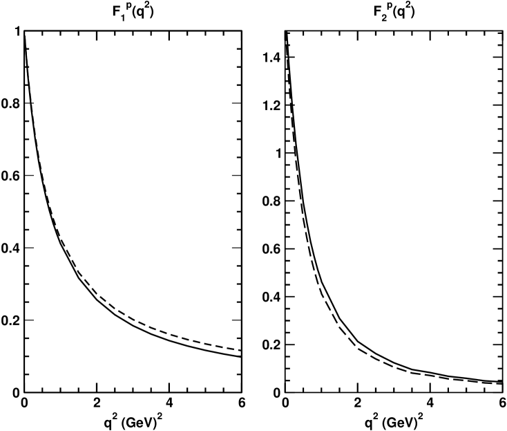
Figure 1: Left panel – Calculated proton Dirac form factor; Right panel – Calculated proton Pauli form factor. Solid line, $\mbox{\sc r}=0.25$; dashed, $\mbox{\sc r}=0.50$. The associated model parameters are listed in Table 3.

In Table 3 we list the parameter values produced by this fitting procedure along with the calculated values of proton and neutron static properties. The proton’s charge radius is precisely that for which we aimed. However, the remaining values point to the deficiencies of a model that retains only a scalar diquark correlation. They confirm that in this case one is unable to obtain a quantitatively accurate picture of the nucleon. This is reassuring because, in contributing to nucleon observables, axial-vector diquark correlations primarily interfere constructively with the pion cloud; e.g., they both provide additional binding and hence act to reduce the nucleon’s mass [25], and they both act to increase $|\mu_{p,n}|$, $|r_{p,n}^{2}|$ [12, 55, 56, 57]. Hence a model that ignores these contributions but succeeds in fitting experimental data is likely to possess spurious degrees of freedom. The improvements necessary to make the model more realistic are therefore plain. In their absence it is nevertheless possible to illustrate important points.

A first observation relates to what may be called the nucleon’s “quark core.” In an internally consistent model it is always possible to identify the relative strength of various contributions to a physical observable. For example, Ref. [25] employs a rainbow-dressed quark and ladder-bound meson basis, within which the quark core contributes approximately 85% of the nucleon’s mass. In the present case an estimate of the core’s spatial extent is afforded by $l_{q\{qq\}}=1/\omega_{q\{qq\}}\approx\frac{2}{3}\,$fm, which is commensurate with our calculated core contribution to the proton’s charge radius, Table 3. It will also be evident that this scale is consistent with estimates of the magnitude of meson-loop contributions to the proton’s charge radius determined from lattice-QCD simulations [55, 57].

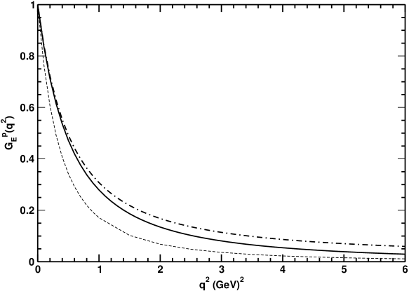
Figure 2: Calculated proton electric form factor: solid line, $\mbox{\sc r}=0.25$; dot-dashed, $\mbox{\sc r}=0.50$ – the associated model parameters are listed in Table 3. For comparison, the lighter dashed line is $G_{E}^{p}(q^{2})=1/(1+q^{2}/m_{\rm emp-p}^{2})^{2}$, $m_{\rm emp-p}=0.84\,$GeV; viz., a dipole fit to available proton data.

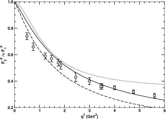
Figure 3: Calculated ratio $F_{2}^{p}/(\kappa F_{1}^{p})$, $\kappa=\mu_{p}-1$: solid line, $\mbox{\sc r}=0.25$; dashed, $\mbox{\sc r}=0.50$ – the associated model parameters are listed in Table 3. The short-dashed line was obtained with the model parameters in Ref. [10]: $\mbox{\sc r}=0.0$, and (in GeV) $m_{0^{+}}=0.63$, $\omega_{0^{+}}=1.0$, $\omega_{q\{qq\}}=0.2$. Data: boxes, Ref.[29]; circles, Ref.[31].

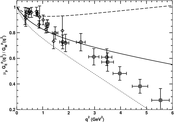
Figure 4: Calculated ratio $\mu_{p}G_{E}^{p}(q^{2})/G_{M}^{p}(q^{2})$: solid line, $\mbox{\sc r}=0.25$; dashed, $\mbox{\sc r}=0.50$ – the associated model parameters are listed in Table 3. The lighter short-dashed line was obtained with the model parameters in Ref. [10]: $\mbox{\sc r}=0.0$, and (in GeV) $m_{0^{+}}=0.63$, $\omega_{0^{+}}=1.0$, $\omega_{q\{qq\}}=0.2$. Data: boxes, Ref.[29]; diamonds, Ref.[30]; circles, Ref.[31].

We depict the proton’s Dirac form factor in the left panel of Fig. 1, wherein it is clear that the shift in parameter values has little observable impact. That is also true for the Pauli form factor, which is plotted in the right panel. These two functions together give the proton’s electric form factor, via Eq. (21), and that is shown in Fig. 2.

We plot the calculated ratio: $F_{2}/\kappa\,F_{1}$, $\kappa=\mu_{p}-1$, in Fig. 3, along with modern experimental data [29, 31]. In addition, we draw the calculated result for this ratio obtained using the parameter values of the scalar diquark Ansatz employed in Ref. [10]. These values: $\mbox{\sc r}=0.0$, and (in GeV) $m_{0^{+}}=0.63$, $\omega_{0^{+}}=1.4$, $\omega_{q\{qq\}}=0.2$, were fixed via a least-squares fit to Eq. (22) but with $m_{d}=0.84\,$GeV, which gives $r_{p}=0.87\,$fm. The figure illustrates that the ratio decreases smoothly with increasing r, bracketing the data, and thereby suggests that even the rudimentary Ansatz is capable of accurately describing the data. Indeed, the $\mbox{\sc r}=0.25$ parameter set might even be considered a good representation. However, this is not the conclusion we draw. Rather, the result demonstrates that the available data on this ratio is sensitive to model-dependent details.

The ratio $\mu_{p}G_{E}^{p}/G_{M}^{p}$ is depicted in Fig. 4 and therein the last statement is amplified. The proton’s electric form factor is a difference, Eq. (21), and that accentuates its sensitivity. On the domain for which data is available, this ratio is particularly responsive to model details, a result also conspicuous in Ref. [12]. It is plain that three parameter sets, which are reasonable and differ modestly when compared through the ratio $F_{2}/\kappa\,F_{1}$, appear vastly different in the comparison presented in Fig. 4. Moreover, because of continuity, it is clear that one could tune the model parameters to fit the data on this ratio. However, what might be considered success in that endeavour could easily be achieved through results for $G_{E}^{p}$ and $G_{M}^{p}$ individually which both disagree with the data.

4 Summary and Discussion

We calculated the proton’s elastic electromagnetic form factors using a rudimentary Ansatz for the nucleon’s Poincaré covariant Faddeev amplitude that represents the proton as a composite of a confined quark and confined nonpointlike scalar diquark. All such models give a Faddeev wave function that corresponds to a nucleon spinor with a sizeable lower component in the rest frame.

This study indicates that on the domain of $q^{2}$ accessible in modern precision experiments these form factors are a sensitive probe of nonperturbative dynamics. The calculated pointwise forms express a dependence on the length-scales that characterise nonperturbative phenomena, such as bound state extent, dressing of quark and gluon propagators, and meson cloud effects. This is precisely analogous to the current status of the pion’s electromagnetic form factor, for which the behaviour predicted in a straightforward application of perturbative QCD is not unambiguously evident until $q^{2}\gtrsim 15\,$GeV² [35].

The ratio $\mu_{p}G_{E}^{p}/G_{M}^{p}$ is particularly sensitive to infrared dynamics because, as $q^{2}$ increases, $G_{E}^{p}(q^{2})$ is a difference of small quantities. However, this ratio should not be considered in isolation because it is possible to reproduce the experimental data using a model that simultaneously provides a poor description of the individual form factors. That is also true of the ratio $F_{2}^{p}/\kappa F_{1}^{p}$ but this combination is less responsive to model particulars because the Dirac and Pauli form factors are positive and fall uniformly to zero, with a momentum dependence at asymptotically large momenta given by perturbative QCD [59, 60]. In the absence of a veracious theoretical understanding of the nucleon, we view the latter ratio as a more sensible constraint on contemporary studies.

It is apparent that much can be learnt about long-range dynamics in QCD from existing and forthcoming accurate data on nucleon form factors. In constraining systematic QCD-based calculations, one can hope, for example, to see an evolution from the domain on which meson cloud effects are important to that whereupon observables are dominated by the confined quark core. This could be elucidated by improving the present study; viz., basing it on a solution of the Poincaré covariant Faddeev equation with axial-vector diquark correlations, instead of using an Ansatz for the Faddeev amplitude, and explicitly including meson cloud contributions. The form factors would then be tied directly to assumptions about the nature of quark-gluon dynamics in the nucleon.

We are grateful to M. B. Hecht for helpful correspondence and for providing us with his computer code; and to F. Coester and T.-S. H. Lee for constructive discussions. This work was supported by: the Department of Energy, Nuclear Physics Division, under contract no. W-31-109-ENG-38; the Austrian Research Foundation FWF under Erwin-Schrödinger-Stipendium no. J2233-N08; and benefited from the resources of the National Energy Research Scientific Computing Center.

Appendix A Nucleon-Photon Vertex

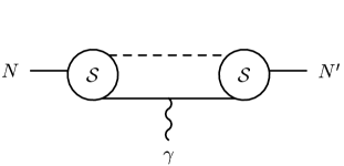
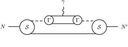
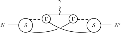
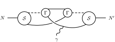
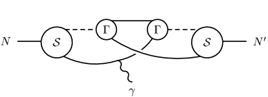
Figure 5: One-body current obtained from the product Ansatz of Eq. (9). Solid line, dressed-quark propagator $S(p)$; dashed line, diquark propagator $\Delta^{0^{+}}(K)$. The amputated nucleon vertex is $\Psi_{3}^{0^{+}}\!\!$ in every case.

We use an Ansatz for $\Psi_{3}$ in the nucleon’s Faddeev amplitude, Eq. (13), from which a properly antisymmetrised one-body vertex can be constructed via the method outlined in Ref. [4]:

$$\Lambda_{\mu}(q,P) = \Lambda^{1}_{\mu}(q,P)+2\sum_{i=2}^{5}\,\Lambda^{i}_{\mu}(q,P)\,,$$ (23)

wherein:

$$\Lambda^{1}_{\mu}(q,P)=3\int\!\!\mbox{\footnotesize$\displaystyle\frac{d^{4}\ell}{(2\pi)^{4}}$}\,{\cal S}(\ell-\mbox{\footnotesize$\displaystyle\frac{2}{3}$}q;P)\,\Delta^{0^{+}}(K)\,{\cal S}(\ell;P)\,\Lambda_{\mu}^{S}(p_{3}+q,p_{3})\,,$$ (24)

with $K=\ell+\mbox{\footnotesize$\displaystyle\frac{2}{3}$}P$, $p_{3}=\mbox{\footnotesize$\displaystyle\frac{1}{3}$}P-\ell$, $\Lambda_{\mu}^{S}(\ell_{1},\ell_{2})=S(\ell_{1})\,\Gamma_{\mu}^{Q}(\ell_{1},\ell_{2})\,S(\ell_{2})$; and

$$\Lambda^{2}_{\mu}(q,P)=6\int\!\!\mbox{\footnotesize$\displaystyle\frac{d^{4}k}{(2\pi)^{4}}$}\mbox{\footnotesize$\displaystyle\frac{d^{4}\ell}{(2\pi)^{4}}$}\,\Omega(p_{1}+q,p_{2},p_{3})\,\Omega(p_{1},p_{2},p_{3})\,{\rm tr}_{DF}\left[\Lambda_{\mu}^{S}(p_{1}+q,p_{1})S(p_{2})\right]\,S(p_{3})\,,$$ (25)

where $p_{1}=\mbox{\footnotesize$\displaystyle\frac{1}{2}$}K+k$, $p_{2}=\mbox{\footnotesize$\displaystyle\frac{1}{2}$}K-k$, $6=\varepsilon_{c_{1}c_{2}c_{3}}\varepsilon_{c_{1}c_{2}c_{3}}$ is the colour contraction, and

$$\Omega(p_{1},p_{2},p_{3})=\Delta^{0^{+}}(p_{\{12\}})\,\Gamma_{0^{+}}(\mbox{\footnotesize$\displaystyle\frac{1}{2}$}p_{[12]};p_{\{12\}})\,{\cal S}(\mbox{\footnotesize$\displaystyle\frac{1}{3}$}[p_{\{12\}}-2p_{3}];P)\,.$$ (26)

$\Lambda_{\mu}^{2}$ describes the photon probing the structure of the scalar diquark correlation, and contributes equally to both the proton and neutron. The remaining terms are

$$\Lambda^{3}_{\mu}(q,P)=6\int\!\!\mbox{\footnotesize$\displaystyle\frac{d^{4}k}{(2\pi)^{4}}$}\mbox{\footnotesize$\displaystyle\frac{d^{4}\ell}{(2\pi)^{4}}$}\,\Omega(p_{1},p_{2},p_{3})\,$$ (27)

$$\times\,\Omega(p_{1}+q,p_{3},p_{2})\,S(p_{2})\,(i\tau_{2})^{\rm t}\Lambda^{S}_{\mu}(p_{1},p_{1}+q)\,(i\tau_{2})\,S(p_{3})\,,$$

where “t” denotes matrix transpose, and

$$\Lambda^{4}_{\mu}(q,P) = 6\int\mbox{\footnotesize$\displaystyle\frac{d^{4}k}{(2\pi)^{4}}$}\mbox{\footnotesize$\displaystyle\frac{d^{4}\ell}{(2\pi)^{4}}$}\,\Omega(p_{1},p_{3},p_{2}+q)\,\Omega(p_{1},p_{2},p_{3})\,\Lambda^{S}_{\mu}(p_{2}+q,p_{2})\,S(p_{1})\,S(p_{3})\,,$$

$$\Lambda^{5}_{\mu}(q,P) = 6\int\mbox{\footnotesize$\displaystyle\frac{d^{4}k}{(2\pi)^{4}}$}\mbox{\footnotesize$\displaystyle\frac{d^{4}\ell}{(2\pi)^{4}}$}\,\Omega(p_{1},p_{3}+q,p_{2})\Omega(p_{1},p_{2},p_{3})\,S(p_{2})\,S(p_{1})\,\Lambda_{\mu}^{S}(p_{3}+q,p_{3})\,.$$

We illustrate these five terms in Fig. 5. They are in one-to-one correspondence with those considered in Ref. [58], with the bottom two diagrams, representing $\Lambda_{\mu}^{4,5}$, being progenitors of the “seagull” terms exploited therein to ensure current conservation.

Our results are obtained by evaluating these integrals using Monte-Carlo methods and the input specified in Eqs. (2), (3), (11), (12), (15) and (17).

References

- [1] G. Martinelli and C. T. Sachrajda, Nucl. Phys. B 306, 865 (1988).
- [2] T. Draper, R. M. Woloshyn, W. Wilcox and K. F. Liu, Nucl. Phys. B 318, 319 (1989).
- [3] J. van der Heide, M. Lutterot, J. H. Koch and E. Laermann, “The pion form factor in improved lattice QCD,” hep-lat/0303006.
- [4] C. D. Roberts and S. M. Schmidt, Prog. Part. Nucl. Phys. 45, S1 (2000).
- [5] R. Alkofer and L. v. Smekal, Phys. Rept. 353, 281 (2001).
- [6] P. Maris and C. D. Roberts, “Dyson-Schwinger equations: A tool for hadron physics,” nucl-th/0301049, to appear in Int. J. Mod. Phys. E.
- [7] P. Maris and P. C. Tandy, Phys. Rev. C 61, 045202 (2000).
- [8] G. Martinelli and C. T. Sachrajda, Nucl. Phys. B 316, 355 (1989).
- [9] M. Göckeler, et al., “Nucleon electromagnetic form factors on the lattice and in chiral effective field theory,” hep-lat/0303019.
- [10] J. C. R. Bloch, C. D. Roberts, S. M. Schmidt, A. Bender and M. R. Frank, Phys. Rev. C 60, 062201 (1999).
- [11] J. C. R. Bloch, C. D. Roberts and S. M. Schmidt, Phys. Rev. C 61, 065207 (2000).
- [12] M. Oettel, R. Alkofer and L. v. Smekal, Eur. Phys. J. A 8, 553 (2000).
- [13] P. L. Chung and F. Coester, Phys. Rev. D 44, 229 (1991).
- [14] F. Coester, Prog. Part. Nucl. Phys. 29, 1 (1992).
- [15] E. Pace, G. Salme and A. Molochkov, Nucl. Phys. A 699, 156 (2002).
- [16] S. Boffi, et al., Eur. Phys. J. A 14, 17 (2002).
- [17] G. A. Miller and M. R. Frank, Phys. Rev. C 65, 065205 (2002).
- [18] R. T. Cahill, C. D. Roberts and J. Praschifka, Phys. Rev. D 36, 2804 (1987).
- [19] P. Maris, Few Body Syst. 32, 41 (2002).
- [20] M. Hess, F. Karsch, E. Laermann and I. Wetzorke, Phys. Rev. D 58, 111502 (1998).
- [21] A. Bender, C. D. Roberts and L. v. Smekal, Phys. Lett. B 380, 7 (1996).
- [22] G. Hellstern, R. Alkofer and H. Reinhardt, Nucl. Phys. A 625, 697 (1997).
- [23] A. Bender, W. Detmold, C. D. Roberts and A. W. Thomas, Phys. Rev. C 65, 065203 (2002).
- [24] R. T. Cahill, C. D. Roberts and J. Praschifka, Austral. J. Phys. 42, 129 (1989).
- [25] M. B. Hecht, M. Oettel, C. D. Roberts, S. M. Schmidt, P. C. Tandy and A. W. Thomas, Phys. Rev. C 65, 055204 (2002).
- [26] M. Oettel, G. Hellstern, R. Alkofer and H. Reinhardt, Phys. Rev. C 58, 2459 (1998).
- [27] E. J. Brash, A. Kozlov, S. Li and G. M. Huber, Phys. Rev. C 65, 051001 (2002).
- [28] J. Arrington, “How well do we know the electromagnetic form factors of the proton?,” nucl-ex/0305009.
- [29] M. K. Jones et al. [JLab Hall A Collaboration], Phys. Rev. Lett. 84, 1398 (2000).
- [30] O. Gayou, et al., Phys. Rev. C 64, 038202 (2001).
- [31] O. Gayou, et al. [JLab Hall A Collaboration], Phys. Rev. Lett. 88, 092301 (2002).
- [32] T. Gousset, B. Pire and J. P. Ralston, Phys. Rev. D 53, 1202 (1996).
- [33] P. Maris, C. D. Roberts and P. C. Tandy, Phys. Lett. B 420, 267 (1998).
- [34] G. R. Farrar and D. R. Jackson, Phys. Rev. Lett. 43, 246 (1979).
- [35] P. Maris and C. D. Roberts, Phys. Rev. C 58, 3659 (1998).
- [36] P. O. Bowman, U. M. Heller and A. G. Williams, Phys. Rev. D 66, 014505 (2002).
- [37] M. S. Bhagwat, M. A. Pichowsky, C. D. Roberts and P. C. Tandy, “Analysis of a quenched lattice-QCD dressed-quark propagator,” nucl-th/0304003, to appear in Phys. Rev. C.
- [38] P. Maris and C. D. Roberts, Phys. Rev. C 56, 3369 (1997).
- [39] C. J. Burden, C. D. Roberts and M. J. Thomson, Phys. Lett. B 371, 163 (1996).
- [40] S. Capstick and W. Roberts, Prog. Part. Nucl. Phys. 45, S241 (2000).
- [41] M. B. Hecht, C. D. Roberts and S. M. Schmidt, Phys. Rev. C 64, 025204 (2001).
- [42] M. Bando, M. Harada and T. Kugo, Prog. Theor. Phys. 91, 927 (1994).
- [43] C. D. Roberts, Nucl. Phys. A 605, 475 (1996).
- [44] R. Alkofer and C. D. Roberts, Phys. Lett. B 369, 101 (1996).
- [45] D. Kekez and D. Klabučar, Phys. Lett. B 457, 359 (1999).
- [46] C. D. Roberts, Fizika B 8, 285 (1999).
- [47] P. C. Tandy, Fizika B 8, 295 (1999).
- [48] A. Bashir, A. Kızılersü and M. R. Pennington, Phys. Rev. D 57, 1242 (1998).
- [49] A. Bashir, A. Kızılersü and M. R. Pennington, “Analytic form of the one-loop vertex and of the two-loop fermion propagator in 3-dimensional massless QED,” hep-ph/9907418.
- [50] J. Volmer, et al. [JLab Collaboration], Phys. Rev. Lett. 86, 1713 (2001).
- [51] J. S. Ball and T.-W. Chiu, Phys. Rev. D 22, 2542 (1980).
- [52] M. A. Pichowsky, S. Walawalkar and S. Capstick, Phys. Rev. D 60, 054030 (1999).
- [53] R. Alkofer, A. Bender and C. D. Roberts, Int. J. Mod. Phys. A 10, 3319 (1995).
- [54] F. Cardarelli, E. Pace, G. Salme and S. Simula, Phys. Lett. B 357, 267 (1995).
- [55] D. B. Leinweber and T. D. Cohen, Phys. Rev. D 47, 2147 (1993).
- [56] E. J. Hackett-Jones, D. B. Leinweber and A. W. Thomas, Phys. Lett. B 489, 143 (2000).
- [57] E. J. Hackett-Jones, D. B. Leinweber and A. W. Thomas, Phys. Lett. B 494, 89 (2000).
- [58] M. Oettel, M. A. Pichowsky and L. v. Smekal, Eur. Phys. J. A 8, 251 (2000).
- [59] G. P. Lepage and S. J. Brodsky, Phys. Rev. Lett. 43, 545 (1979) [Erratum-ibid. 43, 1625 (1979)].
- [60] G. P. Lepage and S. J. Brodsky, Phys. Rev. D 22, 2157 (1980).