A Multi-Shell Shell Model for Heavy Nuclei

Abstract

Performing a shell model calculation for heavy nuclei has been a long-standing problem in nuclear physics. Here we propose one possible solution. The central idea of this proposal is to take the advantages of two existing models, the Projected Shell Model (PSM) and the Fermion Dynamical Symmetry Model (FDSM), to construct a multi-shell shell model. The PSM is an efficient method of coupling quasi-particle excitations to the high-spin rotational motion, whereas the FDSM contains a successful truncation scheme for the low-spin collective modes from the spherical to the well-deformed region. The new shell model is expected to describe simultaneously the single-particle and the low-lying collective excitations of all known types, yet keeping the model space tractable even for the heaviest nuclear systems.

I Introduction

Except for a few nuclei lying in the vicinity of shell closures, most of the heavy nuclei are difficult to describe in a spherical shell model framework because of the unavoidable problem of dimension explosion. Therefore, the study of nuclear structure in heavy nuclei has relied mainly on the mean-field approximations, in which the concept of spontaneous symmetry breaking is applied RS80 ; Frau01 . However, there has been an increasing number of compelling evidences indicating that the nuclear many-body correlations are important. Thus, the necessity of a proper quantum mechanical treatment for nuclear states has been growing, and we are facing the challenge of understanding the nuclear structure by going beyond the mean-field approximations.

Demand for a proper shell model treatment arises also from the nuclear astrophysics. Since heavy elements are made in stellar evolution and explosions, nuclear physics, and in particular nuclear structure far from stability, enters into the stellar modeling in a crucial way. The nucleosynthesis and the correlated energy generation is not completely understood, and the origin of elements in the cosmos remains one of the biggest unsolved physics puzzles. Nuclear shell models can generate well-defined wave functions in the laboratory frame, allowing us to compute, without further approximations as often assumed in the mean-field approaches, the quantities such as transition probabilities, spectroscopic factors, and $\beta$-decay rates. These quantities provide valuable structure information to nuclear astrophysics. In fact, the nuclear shell model calculations could strongly modify the results of nuclear astrophysics, as the recent work of Langanke and Martinez-Pinedo has demonstrated (see, for example, Ref. LM00 ).

Tremendous efforts have been devoted to extending the shell model capacity from its traditional territory of the $sd$-shell to heavier shells. Over the years, one has looked for possible solutions in the following two major directions. In the first direction, one employs rapidly growing computer power and sophisticated diagonalization algorithms to improve the traditional shell model code. The shell model code ANTOINE Caurier1 is a representative example of the recent developments along this line. Using this code the deformed $N\approx Z$ nuclei up to mass $A\sim 50$ can be well explained. The recent record example performed by this code is the full $fp$ shell calculation of $A=52$ nuclei ur , with the basis dimensions in excess of 100 million.

While in principle, it does not matter how to prepare a shell model basis, it is crucial in practice to use the most efficient one. Moreover, feasibility in computation is not our only concern. The other important aspect of using an efficient basis is that it may have a good classification scheme, such that a simple configuration in that basis corresponds approximately to a real mode of excitation. This not only can simplify the calculations, but also make the physical interpretations of results more easy and transparent.

In the second direction, which is defined in a much wider scope, one employs various methods in seeking judicious truncation schemes. Such schemes should contain the most significant configurations, each of which can be a complicated combination in terms of the original shell model basis states. In this way, the basis dimension can be significantly reduced and the final diagonalization is performed in a much smaller space, thus making a shell model calculation for heavy nuclei possible. The early MONSTER-VAMPIRE approach MV and the recent Monte Carlo Shell Model honma ; MC are examples along this line. Nevertheless, numerical calculations required by these models are still quite heavy, which may make a systematical application difficult.

There are two other existing models that belong to the second category: the Project Shell Model (PSM) psm , and the Fermion Dynamical Symmetry Model (FDSM) fdsm . In the PSM, the shell model basis is constructed by choosing a few quasi-particle (qp) orbitals near the Fermi surfaces and performing angular-momentum and particle-number projection on the chosen configurations. By taking multi-qp states as the building blocks, the PSM has been designed to describe the rotational bands built upon qp excitations psm . The PSM has been rather successful in calculating the high-spin states of well-deformed and superdeformed nuclei. For lighter nuclei where the large-scale shell model calculation is feasible Caurier2 , studies for the deformed ⁴⁸Cr HSM99 and the superdeformed ³⁶Ar LS01 have demonstrated that the PSM calculation can achieve a similar accuracy in describing the data. In the FDSM, the truncated basis is built by the symmetry detected $S$- and $D$-pairs, assuming that these are the relevant degrees of freedom for the low-lying collective motions. Having these pairs as the building blocks, the FDSM can provide a unified description for the low-spin collective excitations from the spherical to the well-deformed region fdsm .

It is clear that the PSM and the FDSM follow the shell model philosophy and both have their own shell model truncation scheme. However, the truncations emphasize different excitation modes, which are contained in one model but are absent in the other. An idea emerges naturally that one may combine the advantages of the two models to construct a new shell model for heavy nuclei. The question is how. The PSM is a microscopic approach employing the deformed intrinsic states and the projection method, while the FDSM is a fermionic model based on the group theory. The crucial step that leads us to connect these two different approaches is made through the recent recognition psmsu3 ; psmsu3b that the numerical results obtained by the PSM exhibit, up to high angular momenta and excitations, a remarkable one-to-one correspondence with the analytical $SU(3)$ spectrum of the FDSM. This suggests that the projected deformed-BCS vacuum has at the microscopic level $SU(3)$-like structures which are very close to the representations of the $SU(3)$ dynamical symmetry of an $S$-$D$ fermion-pair system. This recognition has motivated us to propose a multi-shell shell model for heavy nuclei. Hereafter, we shall call it Heavy Shell Model, or HSM for short.

In the following section, the PSM and the FDSM will be briefly reviewed. The emphasis will be given on the discussion of the advantages and deficiencies of each model. In Section 3, the connection between the two models will be explored. In Section 4, we will discuss in detail how the two models are integrated to form the HSM. We will give the basis states and the basis truncations for the well-deformed, transitional, and spherical regions. The effective interactions and the general method for evaluating the projected matrix elements will also be discussed in this section. Finally, the paper will be summarized in Section 5.

II Projected Shell Model and Fermion Dynamical Symmetry Model

In this section, we introduce the basic structure of the PSM and the FDSM. For each model, we point out the main features and the limitations. For interested readers, we refer to the review article of the PSM psm and of the FDSM fdsm .

II.1 Projected Shell Model

The PSM begins with the deformed (e.g. the Nilsson-type) single particle basis, with pairing correlations incorporated into the basis by a BCS calculation for the Nilsson states. The basis truncation is first implemented in the multi-qp states with respect to the deformed-BCS vacuum $\left|\Phi\right>$; then the angular-momentum and the particle-number projection are performed on the selected qp basis to form a shell model space in the laboratory frame; finally a shell model Hamiltonian is diagonalized in this projected space.

If $a^{\dagger}_{\nu}$ and $a^{\dagger}_{\pi}$ are the qp creation operators, with the index $\nu_{i}$ ($\pi_{i}$) denoting the neutron (proton) quantum numbers and running over properly selected single-qp states, the multi-qp bases of the PSM are given as follows:

even-even nucleus: $$\{\left|\Phi\right\rangle,\ a^{\dagger}_{\nu_{i}}a^{\dagger}_{\nu_{j}}\left|\Phi\right\rangle,\ a^{\dagger}_{\pi_{i}}a^{\dagger}_{\pi_{j}}\left|\Phi\right\rangle,$$

$$a^{\dagger}_{\nu_{i}}a^{\dagger}_{\nu_{j}}a^{\dagger}_{\pi_{k}}a^{\dagger}_{\pi_{l}}\left|\Phi\right\rangle,\cdots\}$$

odd-$$\nu \{a^{\dagger}_{\nu_{i}}\left|\Phi\right\rangle,\ a^{\dagger}_{\nu_{i}}a^{\dagger}_{\pi_{j}}a^{\dagger}_{\pi_{k}}\left|\Phi\right\rangle,\ \cdots\}$$ nucleus: (1)

odd-$$\pi \{a^{\dagger}_{\pi_{i}}\left|\Phi\right\rangle,\ a^{\dagger}_{\pi_{i}}a^{\dagger}_{\nu_{j}}a^{\dagger}_{\nu_{k}}\left|\Phi\right\rangle,\cdots\}$$ nucleus:

odd-odd nucleus: $$\{a^{\dagger}_{\nu_{i}}a^{\dagger}_{\pi_{j}}\left|\Phi\right\rangle,\cdots\}$$

In bases (1), “$\cdots$” denotes those configurations that contain more than two like-nucleon quasi-particles. If one is interested in the low-lying states only, they can practically be ignored because these configurations have higher excitation energies due to mutual blocking of levels. The bases (1) can be easily enlarged by including higher order of multi-qp states if necessary. If the configurations denoted by “$\cdots$” are completely included, one recovers the full shell model space written in the representation of qp excitation.

In the qp basis, the truncation can now be easily implemented by simply excluding the states with higher energies. Usually, only a few orbitals around the Fermi surfaces are sufficient for a description of the low-lying qp excitations. The truncation is thus so efficient that dimension never poses a problem even for superdeformed, heavy nuclei.

After the truncation is implemented in the multi-qp basis, the shell model space can be constructed by the projection technique RS80 :

$$\left|qKIM\right\rangle=\hat{P}^{IN}_{MK}\left|\Phi_{q}\right\rangle\mbox{\hskip 6.0pt with\hskip 6.0pt $\hat{P}^{IN}_{MK}=\hat{P}^{I}_{MK}\hat{P}^{N}$,}$$ (2)

where $\left|\Phi_{q}\right\rangle$ denotes the qp-basis given in (1) with $q$ meaning the multi-qp configuration, and

$$\hat{P}^{I}_{MK} = \frac{2I+1}{8\pi^{2}}\int d\Omega D^{I}_{MK}(\Omega)\hat{R}(\Omega)$$

$$\hat{P}^{N} = \frac{1}{2\pi}\int d\phi e^{-i(\hat{N}-N)\phi}$$ (3)

are the angular momentum and particle number projection operators, respectively. In Eq. (3), $D^{I}_{MK}$ is the $D$-function BM69 , $\hat{R}$ the rotation operator, $\Omega$ the solid angle, $\hat{N}$ the number operator, and $\phi$ the gauge angle. If one keeps the axial symmetry in the deformed basis, $D^{I}_{MK}$ in Eq. (3) reduces to the small $d$-function and the three dimensions in $\Omega$ reduce to one. The eigen-values $E$ and the corresponding wave functions $\left|\Psi^{I}_{M}\right\rangle=\sum_{qK}F^{I}_{qK}\left|qKIM\right\rangle$ are then obtained by solving the following eigen-value equation:

$$\sum_{qK}\left\{H^{I}_{qK\ q^{\prime}K^{\prime}}-E\ N^{I}_{qK\ q^{\prime}K^{\prime}}\right\}\ F^{I}_{q^{\prime}K^{\prime}}=0,$$ (4)

where $H^{I}_{qK\ q^{\prime}K^{\prime}}$ and $N^{I}_{qK\ q^{\prime}K^{\prime}}$ are respectively the matrix elements of the Hamiltonian and the norm

$$\begin{array}[]{l}H^{I}_{qK\ q^{\prime}K^{\prime}}\equiv\langle qKI|\hat{H}|q^{\prime}K^{\prime}I\rangle=\langle\Phi_{q}|\hat{H}\hat{P}^{IN}_{KK^{\prime}}|\Phi_{q^{\prime}}\rangle\vspace{+8pt}\\ N^{I}_{qK\ q^{\prime}K^{\prime}}\equiv\hskip 6.0pt\langle qKI|q^{\prime}K^{\prime}I\rangle\hskip 6.0pt=\hskip 6.0pt\langle\Phi_{q}|\hat{P}^{IN}_{KK^{\prime}}|\Phi_{q^{\prime}}\rangle.\end{array}$$ (5)

The PSM uses a large size of single-particle (s. p.) space, which ensures that the collective motion is defined microscopically by accommodating a sufficiently large number of active nucleons. It usually includes three (four) major shells each for neutrons and protons in a calculation for deformed (superdeformed) nuclei. The effective interactions employed in the PSM are the separable forces. The Hamiltonian takes the following form:

$$\begin{array}[]{l}\hat{H}=\sum_{\sigma=\nu,\pi}\hat{H}_{\sigma}+\hat{H}_{\nu\pi},~{}~{}~{}~{}\hat{H}_{\nu\pi}=-\chi_{\nu\pi}\,{\hat{Q}^{\nu\dagger}_{2}}\cdot\hat{Q}^{\pi}_{2}\vspace{+8pt}\\ \hat{H}_{\sigma}=\hat{H}_{0}^{\sigma}-{\chi_{\sigma}\over 2}{\hat{Q}^{\sigma\dagger}_{2}}\cdot\hat{Q}^{\sigma}_{2}-G^{\sigma}_{\mbox{\scriptsize M}}\hat{P}^{\sigma}{}^{\dagger}\hat{P}^{\sigma}-G^{\sigma}_{\mbox{\scriptsize Q}}{\hat{P}^{\sigma}_{2}}{}^{\dagger}\cdot\hat{P}^{\sigma}_{2}.\end{array}$$ (6)

The first term $\hat{H}^{\sigma}_{0}$ in $\hat{H}_{\sigma}$ of Eq. (6) is the spherical single-particle Hamiltonian and the remaining terms are residual quadrupole-quadrupole, monopole-pairing, and quadrupole-pairing interactions, respectively. The strength of the quadrupole-quadrupole force is determined in a self-consistent way that it would give the empirical deformation as predicted in the variation calculations. The monopole-pairing strength is taken as the form $G_{\mbox{\scriptsize M}}=G/A$ ($A$ is the mass number) with $G$ being adjusted to yield the known odd-even mass differences. The quadrupole-pairing strength $G_{\mbox{\scriptsize Q}}$ is assumed to be about 20$\%$ of $G_{\mbox{\scriptsize M}}$ psm .

The one-body operators (for each kind of nucleons) in Eq. (6) are of the standard form

$$\hat{Q}_{\mu} = \sum_{\alpha,\alpha^{\prime}}\ Q_{\mu\alpha\alpha^{\prime}}\ c^{\dagger}_{\alpha}c_{\alpha^{\prime}}$$

$$\hat{P}^{\dagger} = \frac{1}{2}\sum_{\alpha}c^{\dagger}_{\alpha}c^{\dagger}_{\bar{\alpha}}$$ (7)

$$\hat{P}^{\dagger}_{\mu} = \frac{1}{2}\sum_{\alpha,\alpha^{\prime}}\ Q_{\mu\alpha\alpha^{\prime}}c^{\dagger}_{\alpha}c^{\dagger}_{\bar{\alpha}^{\prime}}$$

where $Q_{\mu\alpha\alpha^{\prime}}=\langle\alpha|\hat{Q}_{2\mu}|\alpha^{\prime}\rangle$ is the one-body matrix element of the quadrupole operator and $c^{\dagger}_{\alpha}$ the nucleon creation operator, with $\alpha$ standing for the quantum numbers of a s. p. state in the spherical basis ($\alpha\equiv\{n\ell jm\}$). The time reversal of $c^{\dagger}_{\alpha}$ is defined as $c_{\bar{\alpha}}\equiv(-)^{j-m}c_{n\ell j-m}$.

For a description of rotational bands associated with a well-deformed minimum, the PSM is a highly efficient truncation scheme. Diagonalization for a heavy nucleus can be done almost instantly, yet the results are often satisfactory. The reason for the success is because the major part of pairing and quadrupole correlations has already been built in the basis through the use of deformed basis and the BCS formalism. Therefore, a small configuration space with a few s. p. orbits around the Fermi surface can already span a very good basis for the low-lying excitations. Note that each of the configurations in the basis is a complex mixture of multi-shell configurations of the spherical shell model space. Although the final dimension of the PSM is small, it is huge in terms of original shell model configurations. In this sense, the PSM is a shell model in a truncated multi-major-shell space.

The pleasant features of the PSM make it a frequently-used model in the high-spin physics. Many applications can be found in the review article psm . The recent publications include the study of superdeformed structure in a wide range of different mass regions Sun95 ; Sun97 ; Sun99 ; Ted02 , the study of the origin of identical bands Sun96 and of the high-K states SSW98 .

While the PSM is an efficient shell model for deformed systems with rotational behavior, it becomes less valid when going to the transitional region, and eventually loses its applicability for spherical nuclei. Moreover, it can not efficiently describe the $\beta$- and $\gamma$-vibrations. Although such collective modes can in principle be obtained by mixing a large amount of excited qp-configurations, it suffers in practice from a similar dimension problem as in conventional shell models. The main reason for these shortcomings is due to the use of the simple BCS-vacuum which contains only the properties of the ground-state rotational band but not those of the collective vibrations.

II.2 Fermion Dynamical Symmetry Model

If we say that the PSM is a shell model in a truncated multi-major-shell space, then the FDSM is a shell model in a truncated one-major-shell space. The truncation is based on the consideration that the like-nucleons prefer to form coherent $S$ (angular-momentum $L=0$) and $D$ ($L=2$) pairs. One may thus assume that a closed subspace built up by these $S$-$D$ pairs is mainly responsible for nuclear low-lying collective motions. Such an $S$-$D$ subspace can be carved out by a symmetry requirement that the $S$ and $D$ creation (annihilation) operators together with necessary minimum amount of number conserving operators form a closed Lie algebra. To this end, a $k$-$i$ basis is introduced (see Ref. fdsm and the references cited therein)

$$b^{\dagger}_{km_{k},\,im_{i}}=\sum_{j}\ c_{km_{k}\,im_{i}}^{\ jm}\ c^{\dagger}_{jm}$$ (8)

where $k$ (pseudo-orbital angular-momentum) and $i$ (pseudo-spin) could be either $k=1$ and $i=$ any half integer, or $i=3/2$ and $k=$ any integer. This basis must uniquely reproduce the normal-parity levels note1 in that shell by $k$-$i$ angular momentum coupling, no more and no less. With this $k$-$i$ basis, the coherent $S$ and $D$ pairs and the multipole operators $P_{r\mu}$, which are necessary in order to form a closed Lie algebra, are found to be as follows note2 :

$$\begin{array}[]{c}S^{\dagger}=\sum_{i}\sqrt{\frac{\Omega_{ki}}{2}}\left[\,b_{ki}^{\dagger}b_{ki}^{\dagger}\,\right]^{00}_{00}\\ \mbox{(for any $k$ and $i$})\end{array},\ \ \Omega_{ki}=\frac{(2k+1)(2i+1)}{2}$$ (9)

$$\begin{array}[]{c}D_{\mu}^{\dagger}=\sum_{i}\sqrt{\frac{\Omega_{ki}}{2}}\left[\,b_{ki}^{\dagger}b_{ki}^{\dagger}\right]^{20}_{\mu 0},\ \ D_{\mu}^{\dagger}=\sum_{i}\sqrt{\frac{\Omega_{ki}}{2}}\left[\,b_{ki}^{\dagger}b_{ki}^{\dagger}\right]^{02}_{0\mu}\\ \mbox{($k$-active: $k=1$)}\hskip 64.0pt\mbox{($i$-active: $i=3/2$)}\end{array}$$ (10)

$$\begin{array}[]{c}P_{r\mu}=\sum_{i}\sqrt{2\Omega_{ki}}\left[\,b_{ki}^{\dagger}\tilde{b}_{ki}\right]^{r0}_{\mu 0},\ P_{r\mu}=\sum_{i}\sqrt{2\Omega_{ki}}\left[\,b_{ki}^{\dagger}\tilde{b}_{ki}\right]^{0r}_{0\mu}\\ \mbox{($k$-active: $k=1$, $r\leq 2$)}\hskip 20.0pt\mbox{($i$-active: $i=3/2$, $r\leq 3$)}\end{array}\hskip 12.0pt$$ (11)

where the symbol $[\ ]$ denotes angular-momentum coupling, and the time reversal is defined as $\tilde{b}_{km_{k}im_{i}}\equiv(-)^{k-m_{k}+i-m_{i}}{b}_{k-m_{k}i-m_{i}}$. The operator set $\{S^{\dagger},S,D^{\dagger}_{\mu},D_{\mu},P_{r\mu}\}$ forms a closed Lie algebra of either $Sp(6)$ ($k$-active) or $SO(8)$ ($i$-active), depending on the level structure of the valence shell fdsm .

Once the $S$-$D$ subspace is carved out, the form of the effective Hamiltonian (restricted to a two-body interaction) in this truncated space is uniquely determined:

$$H = \sum_{\sigma=\nu,\pi}H^{\sigma}+H^{\nu\pi}\ ,\hskip 14.0ptH^{\nu\pi}=-\sum_{r}B_{r}^{\nu\pi}P^{\nu}_{r}\cdot P^{\pi}_{r}$$

$$H^{\sigma} = H^{\sigma}_{0}-G^{\sigma}_{0}S^{\sigma}{}^{\dagger}S^{\sigma}-G^{\sigma}_{2}D^{\sigma}{}^{\dagger}\cdot D^{\sigma}-\sum_{r>0}B_{r}^{\sigma}P^{\sigma}_{r}\cdot P^{\sigma}_{r}$$ (12)

It can be shown that the multipole operators $P_{r}$ with $r=0,1$ are proportional to the number operator in normal parity levels $n_{1}$ and the total angular-momentum $\hat{I}$, respectively, while $P_{2}$ is proportional to the effective quadrupole operator in the truncated space. The term $H^{\sigma}_{0}$ is a quadratic function of valence neutron and proton numbers ($n^{\pi}n^{\nu}$ is included in the n-p interaction $H^{\nu\pi}$). This Hamiltonian (Eq. (12)) looks formally similar to that of the PSM (Eq. (6)) if we assume that only $B_{2}\neq 0$ in the summation. However, one should bear in mind that the FDSM Hamiltonian is written in a truncated one-major shell space and the s. p.  energy splitting within the shell is neglected. This is the price the FDSM has to pay in order to meet the symmetry requirement so that solutions can be obtained with the aid of group theory.

With this Hamiltonian, it can be shown that there exist analytical solutions in various dynamical symmetry limits, each one corresponding to a collective mode known experimentally: the $SU(3)$-limit in the $k$-active shell and the $SO(6)$-limit in the $i$-active shell correspond respectively to rigid and $\gamma$-soft rotors for well deformed nuclei, while the $SU(2)$-limit in the $k$-active shell and the $SO(5)$-limit in the $i$-active shell correspond to a vibrator of spherical nuclei. Since the FDSM contains all major collective modes, the general feature of different collective motions arises naturally as the number of valence nucleons varies; namely, nuclei behave as a spherical vibrator near the closed shell and become a well-deformed rotor around the mid-shell. If the strengths of the Hamiltonian are properly chosen and the s. p.  splitting is taken into account as a perturbation, the FDSM can even quantitatively reproduce the low-lying spectra, B(E2)’s, ground state masses, etc., in a unified manner from the spherical to well-deformed region.

Table 1: The $SU(3)$ irreps in the FDSM and the collective $\beta$-$\gamma$ vibrations. *

* The $SU(3)$ intrinsic states for each of the $\beta$-$\gamma$ vibrational modes are listed in the first column. The second and the third column are the phonon excitation energies and the associated quantum numbers according to the Particle-Rotor Model. The 4th and 5th column are the $SU(3)$ irreps $(\lambda,\mu)$ and the corresponding Young tablets $[\mbox{h}_{1},\mbox{h}_{2},\mbox{h}_{3}]$, respectively. The excitation energies obtained from the FDSM are listed in the last column as $B_{2}\Delta C(\lambda,\mu)$, where $\Delta C(\lambda,\mu)$ is the changes of the expectation values of the $SU(3)$ Casimir operator with respect to the ground state irrep $C(n_{1},0)$, $B_{2}$ is the $n$-$p$ quadrupole interaction strength, and $\hbar\omega\equiv(3/2)\,n_{1}B_{2}$.

Here, it may be appropriate to emphasize one remarkable result of the FDSM: There exists an one-to-one correspondence between the $SU(3)$ irreps and the $\beta$- and $\gamma$-vibrations in deformed nuclei. As one can see from Table I, the $\beta$-$\gamma$ vibrations are microscopically the collective $D$-pair excitations (the $D^{\dagger}_{\pm 1}$ excitations are forbidden by the time reversal symmetry). The anharmonic behavior of the $\beta$-$\gamma$ vibrations is due to the finite particle number effect. In the large $n_{1}$ limit, ignoring $1/n_{1}$, the FDSM reproduces exactly the Particle-Rotor Model results. This means that the FDSM has discovered the relevant fermion degrees of freedom of nuclear collective motions, which are the $S$ and $D$ pairs. The $S$-$D$ subspace is so compact that it never suffers from the dimension explosion even for the heaviest nuclear systems.

While with the $S$-$D$ subspace the FDSM is able to provide a microscopic view to the low-lying collective motions, it has difficulties in describing the qp excitations and the high-spin physics for lack of the s. p. degrees of freedom. In principle, this can be resolved by allowing a few pairs to break. The problem is that once the s. p. degrees of freedom open up, the dimension increases very rapidly. In addition, inclusion of s. p. degrees of freedom results in adding many new terms to the effective Hamiltonian. To pin down so many coupling strengths in the Hamiltonian is a very difficult task, if not impossible. Therefore, even the number of broken pairs is limited to just one for proton and one for neutron, the model could at best be applied to the $fp$ shell nuclei, and could not go any further.

III Connection between PSM and FDSM

Let us summarize our main claims in the last section. Both the PSM and the FDSM are truncated shell model, aiming at grasping the essential ingredients to describe the low-lying physics. However, the emphasis in each model is different, which is reflected in their different truncation schemes. The PSM emphasizes the high-spin description of rotational states built upon qp-excitations associated with a well-deformed minimum, but it is not an efficient method for the collective vibrations. In contrast, the FDSM has a well-defined classification for all known types of collective vibration, ranging from the spherical, via transitional, to the well-deformed region, but it is lack of the necessary degrees of freedom of qp-excitations. Thus, the main advantages of the PSM and the FDSM are mutually complementary to each other.

If we could take the advantages of the PSM and the FDSM and combine them into a single model, the deficiencies of each model will be eliminated. At first glance, it is not obvious how to bridge these two different approaches. In this section, we show that a realization of the combination is possible. The assertion is made based on the recent recognition that an $SU(3)$ symmetry can emerge from the projected deformed-BCS vacuum. Having this as the basis, the full idea of the microscopic classification for the collective vibrations discovered by the FDSM could be adopted by the PSM while the latter keeps its original features in building the shell model configuration space through projection.

III.1 Emergence of $SU(3)$ Symmetry in PSM

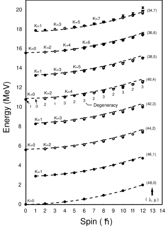
Figure 1: Comparison between the PSM (symbols) and the FDSM $SU(3)$ limits (curves) assuming $n^{\mbox{eff}}_{\nu}=32$ and $n^{\mbox{eff}}_{\pi}=16$. The $SU(3)$ quantum numbers $(\lambda,\mu)\kappa$ are marked for each band with degeneracy of $\kappa=\kappa_{max},\kappa_{max}-2,\cdots,0\mbox{ or }1$, and $\kappa_{max}=min\{\lambda,\mu\}$. The comparison takes the well-deformed nucleus ¹⁶⁸Er as an example.

It is remarkable psmsu3 ; psmsu3b that the states numerically obtained by the PSM exhibit a beautiful one-to-one correspondence with the analytical $SU(3)$ spectrum of the FDSM. To show this, the original PSM was extended in such a way that instead of a single BCS vacuum, the angular momentum projection was performed for separate neutron and proton BCS vacuum with the same deformation, and the projected states were coupled through diagonalization of the Hamiltonian psmsu3 . The extension is necessary; Otherwise the PSM would have no collectively excited bands to compare with the FDSM. This procedure gives the usual rotational ground-band corresponding to a strongly coupled BCS condensate of neutrons and protons, but also led to a new set of excited bands arising from the vibrations of relative orientation of the neutron and proton cores (the so-called “scissors” mode).

As one can see from Fig. 1, the spectrum obtained from the PSM is, up to high angular momenta and excitation energies, nearly identical to that from the FDSM $SU(3)$ formulism with $(n^{\mbox{\scriptsize eff}}_{\nu}=32,0)$ and $(n^{\mbox{\scriptsize eff}}_{\pi}=16,0)$ irreps, respectively assigned to the neutron and proton BCS vacuum. The classification of the spectrum follows exactly the FDSM $SU(3)$ reduction rules

$$(n^{\mbox{\scriptsize eff}}_{\nu},0)\otimes(n^{\mbox{\scriptsize eff}}_{\pi},0)\supset(\lambda,\mu)\ \kappa I$$ (13)

with

$$\lambda = n^{\mbox{\scriptsize eff}}_{\nu}+n^{\mbox{\scriptsize eff}}_{\pi}-2\mu\vspace{4pt}$$

$$\mu = \mu_{\mbox{\scriptsize max}},\mu_{\mbox{\scriptsize max}}-1,\cdots,1,0;\ \ \ \mu_{\mbox{\scriptsize max}}={\mbox{min}}(n^{\mbox{\scriptsize eff}}_{\nu},n^{\mbox{\scriptsize eff}}_{\pi})$$

and

$$\kappa = \kappa_{\mbox{\scriptsize max}},\kappa_{\mbox{\scriptsize max}}-2,\cdots,1\mbox{ or }0;\ \ \ \kappa_{\mbox{\scriptsize max}}={\mbox{min}}(\lambda,\mu)\vspace{4pt}$$

$$I = \left\{\begin{array}[]{l}\lambda+\mu,\lambda+\mu-2,\cdots,1\mbox{ or }0\ ,\ \ \mbox{if }\kappa=0\vspace{4pt}\\ \kappa,\ \kappa+1,\cdots,\lambda+\mu-\kappa+1,\ \ \mbox{if }\kappa\neq 0.\end{array}\right.$$ (16)

Not only the spectrum but also the B(E2)’s exhibit this correspondence psmsu3b . Note that there are many types of $SU(3)$ models, and that different $SU(3)$ models have different permissible irreps and reduction rules due to the different physical input, and therefore can lead to different band structures. Here, we emphasize that this $SU(3)$ symmetry shown in Fig. 1 is of the FDSM type. This is because among the existing fermionic $SU(3)$ models in nuclear physics, only the FDSM $SU(3)$ formulism can naturally provide the required irreps and reproduce the band structure of the PSM. Other $SU(3)$ models such as the pseudo-$SU(3)$ do not have this property. In their recent investigation of the onset of rotational motion, Zuker et. al. qsu3a ; qsu3b introduced a preliminary formulation of an approximate quasi-$SU(3)$ symmetry. It would be interesting to study whether the quasi-$SU(3)$ contains a similar property.

Fig.1 presents a highly non-trivial result because the PSM, as described above, is not built on any explicit $SU(3)$ symmetry, and no free parameters have been adjusted to obtain such a symmetry. Nevertheless, the spectra, the electromagnetic transition rates, and the wave functions of the PSM agree nearly perfectly with the FDSM $SU(3)$ results, from the ground-band to states of high spins and high excitations psmsu3b . This strongly suggests that the projected deformed-BCS vacuum in the PSM could be at the microscopic level close to the $S$-$D$ core in the FDSM, provided that the $S$-$D$ pairs must be redefined in a multi-major-shell space, since the one-major-shell is not large enough to accommodate so many active nucleons (here $n^{\mbox{\scriptsize eff}}_{\nu}=32$ and $n^{\mbox{\scriptsize eff}}_{\pi}=16$).

In this regard, there is a conceptual distinction between the $SU(3)$ symmetry in the one-major-shell FDSM and that emerged from the PSM. In the former, the $SU(3)$ symmetry arises entirely from the normal-parity nucleons, and the abnormal parity orbit enters only implicitly through the Pauli effect and the renormalization of the parameters. In the latter, the $SU(3)$ symmetry arises from the explicit dynamical participation of both normal and abnormal-parity nucleons of many shells. Ignoring the direct contribution from the abnormal-parity nucleons in the one-major-shell FDSM is a sacrifice for having an exact symmetry (which forms a closed Lie algebra). In practice, this turns out to be not a bad approximation for collective motions because in a single major shell, there is only one single-$j$ level with abnormal-parity, which does not have much quadrupole collectivity compared to the normal-parity contributions abnormal . When going to a multi-major-shell space, the situation will change. A bunch of abnormal-parity levels, which are located just below the normal-parity levels, will open up. This means that, when one redefines the FDSM-type coherent $S$-$D$ pairs in a multi-major-shell space, the conceptual distinction of the $SU(3)$ symmetry between the FDSM and the PSM will be eliminated.

III.2 Collective D-Pair Excitations

To see further the relationship between the two models, let us ignore the terms with $r\neq 2$ in the most general FDSM Hamiltonian (12). This is a reasonable approach because from the multipole expansion point of view, there is no multipole interactions with $r=odd$ without considering the parity admixture. One may notice that there is the monopole-monopole interaction ($r=0$) in the FDSM, which is not included in the PSM. However, it is well-known that this interaction only affects the nuclear total binding energy but does not have much influence on the excitations. On the other hand, it can be added to the PSM if necessary. Thus, we have for both models the interactions of the monopole- and quadrupole-pairing plus the quadrupole-quadrupole type.

The PSM Hamiltonian contains operators written in the ordinary shell model basis, whereas the FDSM ones in the $k$-$i$ basis. In order to compare them, we transform the FDSM operators in Eq. (9–11) back to the ordinary shell model basis by rewriting them in terms of $c^{\dagger}_{\alpha}$ and $c_{\alpha}$. We find that

$$P_{2\mu} = \sum_{\alpha,\alpha^{\prime}}\ Q^{(2)}_{\mu\alpha\alpha^{\prime}}\ c^{\dagger}_{\alpha}c_{\alpha^{\prime}}\vspace{2pt}$$

$$S^{\dagger} = \frac{1}{2}\sum_{\alpha}c^{\dagger}_{\alpha}c^{\dagger}_{\bar{\alpha}}\vspace{2pt}$$ (17)

$$D^{\dagger}_{\mu} = \frac{1}{2}\sum_{\alpha,\alpha^{\prime}}\ Q^{(2)}_{\mu\alpha\alpha^{\prime}}c^{\dagger}_{\alpha}c^{\dagger}_{\bar{\alpha}^{\prime}}$$

with

$$Q^{(2)}_{\mu\alpha\alpha^{\prime}} = \sqrt{2\Omega_{ki}}C^{\ 2\mu}_{jm\ j^{\prime}-m^{\prime}}(-)^{r-\mu}\left[\begin{array}[]{lll}i&k&j\\ i&k&j^{\prime}\\ 0&2&2\end{array}\right].$$ (21)

Comparing Eq. (14) with Eq. (7), we see that the definitions of $S^{\dagger}$, $D_{\mu}^{\dagger}$ and $P_{2\mu}$ in the FDSM are similar to that of $\hat{P}^{\dagger}$, $\hat{P}^{\dagger}_{\mu}$ and $\hat{Q}_{\mu}$ in the PSM, except that the model spaces for the two models are different. However, within one-major-shell, the operator $S^{\dagger}$ ($S$) is exactly the same as $P^{\dagger}$ ($P$) in the PSM. For the $D$-pair and $P_{2}$ operators, although the coefficients $Q^{(2)}_{\mu\alpha\alpha^{\prime}}$ look different from $Q_{\mu\alpha\alpha^{\prime}}$ appearing in the corresponding operators $\hat{P}^{\dagger}_{\mu}$ and $\hat{Q}_{\mu}$ in the PSM, their physical meanings are the same. The FDSM Hamiltonian may thus be considered as an one-major-shell version of the PSM Hamiltonian, with the approximations of $\hat{P}^{\dagger}_{\mu}$ and $\hat{Q}_{\mu}$ being replaced by $D_{\mu}^{\dagger}$ and $P_{2\mu}$ and the s. p. energy splitting being ignored. In other words, if, in the multi-major-shell case, the symmetry constraint is released from the FDSM and the s. p. energy splitting is considered, $S^{\dagger}$, $D_{\mu}^{\dagger}$ and $P_{2\mu}$ in the FDSM should return back to the version of $\hat{P}^{\dagger}$, $\hat{P}^{\dagger}_{\mu}$ and $\hat{Q}_{\mu}$ operators in the PSM. So is for the Hamiltonian.

From the above analysis we may conclude that the PSM and the FDSM are just two approaches to solve an effective Hamiltonian of a common form. In order for them to be applicable to heavy nuclei, approximations have to be made in each model. The PSM is based on a multi-major-shell space so that it can describe the nuclear rotational motion microscopically through a dynamic participation of many particles. However, it can afford to do so only for a truncated configuration space that includes only a BCS vacuum plus a few qp excitations. As a sacrifice, this truncation do not include the collective modes such as $\beta$- and $\gamma$-vibrations. In contrast, the FDSM aims at nuclear low-lying collective excitations. It can afford to do so only when the model space is reduced to one-major shell like in the conventional shell model. But that is still not enough for heavy nuclei. Additional approximations to further reduce the configuration space down to the symmetry detected $S$-$D$ subspace are necessary. These approximations exclude the s. p. excitations.

IV Construction of Heavy Shell Model

Having realized that the projected deformed-BCS states exhibit the $SU(3)$ symmetry, and that the collective excitations may be approached by the $D$-pair excitations, with the $D$-pair operator defined as the quadrupole-pair operator $\hat{P}^{\dagger}_{\mu}$ in a multi-major-shell model space, we propose a multi-shell shell model: the Heavy Shell Model. The essence of this proposal is to adopt the truncation scheme for the collective modes, which was discovered by the FDSM, into the PSM to enrich the shell model basis. This essentially combines the advantages of both models.

In fact, to incorporate both s. p.  and collective excitations, there are in principle two alternatives: One can either extend the FDSM by adding the PSM qp truncation scheme on top of the FDSM collective states, or extend the PSM by including the $D$-pair collective excitations into the PSM vacuum. However, the FDSM is a severely truncated one-major-shell shell model dictated by symmetry, and in this sense, it is not as microscopic as the PSM. Although it is quite successful in the description of low-lying collective motions, the FDSM is just an effective theory. For practical applications, large renormalization effects must be embedded in the parameters of the FDSM Hamiltonian, which have to be determined phenomenologically. Therefore, we choose to construct the Heavy Shell Model based on the extension of the PSM.

The main ingredients of the Heavy Shell Model are as follows:

1. Keep the multi-major-shell basis of the PSM as the model space, using the PSM $P^{\dagger}$ and $P_{2}^{\dagger}$ operators to describe the coherent $S$- and $D$-pairs in the multi-major-shell configurations, and construct the intrinsic collective excitation states by $P_{2}^{\dagger}$ acting on the deformed-BCS vacuum;

2. Carry out the shell model truncation by selecting a few single-qp states near the Fermi surfaces plus a few $D$-pair excitations, and perform angular momentum and particle number projection to obtain a shell-model basis in the laboratory frame;

3. Keep the PSM Hamiltonian to be the effective Hamiltonian, but allow adding more multipole interactions and/or readjusting the interaction strengths if necessary;

4. Utilize the algorithms developed in the PSM to carry out calculations for all the necessary matrix elements, and diagonalize the Hamiltonian in the truncated shell model space.

Let us now discuss each of the items in more detail.

IV.1 The Basis States

We have demonstrated that the projected deformed-BCS vacuum $|\Phi\rangle$ in the PSM is nearly identical to the FDSM-$SU(3)$ intrinsic ground state ($n^{\mbox{\scriptsize eff}},0$) irrep. Furthermore, we have indicated that the FDSM $S$- and $D$-pair and the $P_{2\mu}$ operator are, respectively, the symmetry-constraint one-major-shell version of the ordinary monopole pair $P$, quadrupole pair $P_{\mu}$, and quadrupole operator $\hat{Q}_{\mu}$ in the PSM. It is therefore natural to believe that in a multi-major-shell space, the FDSM $S$- and $D$-pairs are nothing but the $P$- and $P_{\mu}$-pairs if we abandon the symmetry requirement. So is for the quadrupole operator. In the FDSM, all known types of low-lying collective excitation can be obtained by acting $D^{\dagger}_{\mu}$ on the FDSM-$SU(3)$ intrinsic ground state, $(S^{\dagger}+\beta D_{0}^{\dagger})^{N}|0\rangle$ (see Table I). Combining these facts, the collective excitations of the HSM in a multi-major-shell space may be constructed by replacing, respectively, $(S^{\dagger}+\beta D_{0}^{\dagger})^{N}|0\rangle$ and $D^{\dagger}$ in Table I with $|\Phi\rangle$ and $P^{\dagger}_{\mu}$ defined in the PSM.

Hereafter, we will continue to use the FDSM notations $S$ and $D$ for the pair operators. One should bear in mind that they have been redefined as

$$S^{\dagger} \equiv P^{\dagger}=\frac{1}{2}\sum_{\alpha}\ c^{\dagger}_{\alpha}c^{\dagger}_{\bar{\alpha}}$$

$$D^{\dagger}_{\mu} \equiv \hat{P}^{\dagger}_{\mu}=\sum_{\alpha,\alpha^{\prime}}\ Q_{\mu\alpha\alpha^{\prime}}\ c^{\dagger}_{\alpha}c^{\dagger}_{\alpha^{\prime}}.$$ (22)

The intrinsic collective states can then be expressed as

$$|\Phi_{c}\rangle \equiv \left|N_{D}(n_{\beta},n_{\gamma},\kappa)\right\rangle=\prod_{i=0}^{N_{D}}D^{\dagger}_{\mu_{i}}|\Phi\rangle\vspace{2pt}$$ (23)

$$= (D^{\dagger}_{0})^{n_{\beta}}(D^{\dagger}_{2}D^{\dagger}_{-2})^{\frac{\mbox{\scriptsize$n$}_{\gamma}}{2}}(D^{\dagger}_{2})^{\frac{\mbox{\scriptsize$\kappa$}}{2}}\left|\Phi\right\rangle.$$

Eq. (23) provides the microscopic meaning of the quantum numbers $n_{\beta}$, $n_{\gamma}$ and $\kappa$ in a very clear manner: the phonon number appearing in phenomenological models is nothing but the total number of $D$-pairs

$$N_{D}=n_{\beta}+n_{\gamma}+\kappa/2.$$ (24)

The basis of the HSM can be constructed by adding qp-excitations on top of the collective intrinsic states; the formalism is the same as that used to build the PSM bases in Eq. (1), but the simple BCS vacuum $|\Phi\rangle$ in Eq. (1) is now replaced by a more correlated one, $|\Phi_{c}\rangle$. The general expression of the HSM basis in the laboratory system can be written as

$$\left|qcIM\right\rangle = \hat{P}^{IN}_{M}\left|\Phi_{qc}\right\rangle\vspace{4pt}$$

$$\left|\Phi_{qc}\right\rangle \equiv \prod_{i=0}^{n^{\nu}_{q}}\prod_{j=0}^{n^{\pi}_{q}}a^{\dagger}_{\nu_{i}}a^{\dagger}_{\pi_{j}}\left|\Phi_{c}\right\rangle,$$ (25)

where $n^{\nu}_{q}$ ($n^{\pi}_{q}$) is the qp number of neutrons (protons), and the indices $q$ and $c$ stand for the qp and the collective vibrational configurations, respectively.

The HSM basis (25) contains both s. p.  (qp excitations) and collective ($D$-pair excitations) degrees of freedom; the deficiency of lack of collective degrees of freedom in the original PSM is redeemed. Moreover, the basis (25) is expected to work also for the transitional (or weakly deformed) nuclei, which is beyond the original PSM territory. This is expected because it is known from the FDSM that the collective states of transitional nuclei can be described as a mixture of different $SU(3)$ irreps fdsm . The original PSM uses only the deformed-BCS vacuum (the ground state of the $SU(3)$ irreps), and thus does not contain such a mixing mechanism. This is why the PSM becomes less and less valid when going away from the well-deformed region. The HSM basis (25) now contains all possible $SU(3)$ irreps, since its labels ($n_{\beta}$, $n_{\gamma}$, $\kappa$) are in one-to-one correspondence to that of the $SU(3)$ irreps $(\lambda,\mu)$ bgvib .

For spherical nuclei, the basis should be constructed separately since in the spherical case, the rotational symmetry is restored so that no distinction can be made between the intrinsic and the laboratory system. In the spherical limit, the BCS vacuum is just the $I=0$ ground state, which, in the FDSM, corresponds to the intrinsic state with $\beta\rightarrow 0$ (see Table II). Let us denote this BCS vacuum as $|\Phi_{0}\rangle$ to distinguish it from the deformed one. The deformed mean-field (e. g.  the Nilsson scheme) in the spherical case is also reduced to the spherical shell model level scheme so that a qp state can be labeled by {$N\ell jm$}. Using {$jm$} for short, a qp state can be expressed as $a^{\sigma}_{j}{}^{\dagger}_{m}|\Phi_{0}\rangle$ ($\sigma=\nu,\pi$), which is no longer a superposition of all possible angular momentum states but has a definite angular momentum. Likewise, a $D$-pair excited state $D^{\dagger}_{\mu}\left|\Phi_{0}\right\rangle$ is now a $2^{+}$ state. Therefore, there is no need for performing angular-momentum projection. The basis with a given total angular-momentum $I$ can be directly obtained by the angular-momentum coupling. The general expression of the HSM basis in the spherical case can be written as follows:

$$\left|qcIM\right\rangle = \hat{P}^{N}\left|\Phi^{IM}_{qc}\right\rangle\vspace{2pt}$$

$$\left|\Phi^{IM}_{qc}\right\rangle \equiv \left[{\bf A}^{\dagger}_{J_{q}}(n_{q})\otimes{\bf D}^{\dagger}_{R_{c}}(N_{D})\right]^{I}_{M}\left|\Phi_{0}\right\rangle$$ (26)

with

$${\bf A}^{\dagger}_{J_{q}M_{q}}(n_{q})\hskip 7.0pt\equiv\left[A^{\dagger}_{J_{q}^{\nu}}(n^{\nu}_{q})\otimes A^{\dagger}_{J_{q}^{\pi}}(n^{\pi}_{q})\right]^{J_{q}}_{M_{q}}\vspace{-12pt}$$ (27)

$$A^{\dagger}_{J_{q}^{\sigma}M_{q}^{\sigma}}(n^{\sigma}_{q})\equiv\mbox{\Large$[$}\prod_{i=1}^{n^{\sigma}_{q}}a^{\dagger}_{j_{i}}\mbox{\Large$]$}^{J^{\sigma}_{q}}_{M^{\sigma}_{q}}=\sum_{[m]}C_{[m]}({J_{q}^{\sigma}M_{q}^{\sigma}})\prod_{i=1}^{n^{\sigma}_{q}}a^{\dagger}_{j_{i}m_{i}}\hskip 4.0pt$$ (28)

$${\bf D}^{\dagger}_{R_{c}M_{c}}(N_{D})\equiv\mbox{\Large$[$}\prod_{k=1}^{N_{D}}D^{\dagger}\mbox{\Large$]$}^{R_{c}}_{M_{c}}=\sum_{[\mu]}C_{[\mu]}(R_{c}M_{c})\prod_{k=1}^{N_{D}}D^{\dagger}_{\mu_{k}}\hskip 6.0pt$$ (29)

where $A^{\dagger}_{J_{q}^{\sigma}M_{q}^{\sigma}}(n^{\sigma}_{q})$ and ${\bf D}^{\dagger}_{R_{c}M_{c}}(N_{D})$ are the creation operators of $n^{\sigma}_{q}$ qp’s and $N_{D}$ $D$-pairs coupled to angular-momenta ${J_{q}^{\sigma}M_{q}^{\sigma}}$ and $R_{c}M_{c}$, respectively. The short-hand notation $[m]$ represents the configuration $\{m_{1},m_{2},\cdots,m_{n^{\sigma}_{q}}\}$ of the qp’s. Similarly, $[\mu]$ is for the $D$-pairs.

Table 2: Comparison of collective basis for deformed and spherical Nuclei. *

* The first column lists the FDSM $SU(3)$ intrinsic states. The second column is the HSM collective basis for the deformed nuclei, which is obtained by replacing $(S^{\dagger}+\beta D^{\dagger}_{0})^{N}|0\rangle$ with the BCS vacuum $|\Phi\rangle$. After projection, each intrinsic state produces a rotational band labeled as $\beta$, $\gamma$, and $(n_{\gamma},n_{\beta},\kappa/2)$ listed in the third column. The FDSM $SU(2)$ states and the HSM collective basis for spherical nuclei are listed in the 4th and 5th column, respectively. The last column lists their corresponding spin-parity and excitation energies relative to the BCS vacuum. Note that the $D$-pairs in the $SU(2)$ states have been modified to commute with $S^{\dagger}$ fdsm .

The amplitudes $C_{[m]}({J_{q}^{\sigma}M_{q}^{\sigma}})$ in Eq. (28) can be easily calculated by using the standard shell model technique. As a matter of fact, all spherical nuclei lie very close to the doubly closed shell. Therefore, only a few qp’s from the $j$-orbits around the Fermi surfaces need to be considered. The amplitudes $C_{[\mu]}(R_{c}M_{c})$ in Eq. (29) are difficult to obtain in this way because multi-major shells are involved due to the $D$-pair collectivity. However, they can be easily evaluated through the $d$-boson CFP’s (Coefficients of Fractional Parentage) if the $D$-pairs are regarded as bosons. It should be noted that this is not a boson approximation since the $D^{\dagger}_{\mu}$’s in Eq. (29) remain to be fermionic operators. It is just a symmetry detected truncation to select only those states that are symmetric with respect to interchanging any $D$-pairs.

A comparison between the deformed basis and the spherical basis is shown in Table II. It is interesting to see that the $D$-pair excited states, which, in the deformed case, produce the $\beta$-$\gamma$ bands after angular-momentum projection, degenerate in the spherical case into a spherical vibration-spectrum. The spherical vibration-spectrum has much less independent states than the rotational spectrum. It is so simply because when $\beta\rightarrow 0$, most of the states obtained from the angular-momentum projection are not linearly independent due to the spherical symmetry nature. They are highly over-complete. For instance, the $\beta$- and $\gamma$-bands reduce to a $2^{+}$ state when $\beta\rightarrow 0$. This is why we should construct the spherical shell-model basis differently. It can be seen that even without configuration mixing, this collective basis (as shown in Table II) can already give the essential features of the low-lying collective modes found in the spherical nuclei. We therefore feel confident that the HSM basis is going to work well.

Of course, having built a shell-model basis is not enough. The central theme that follows is whether it is possible to find an efficient truncation scheme within the constructed basis so that the calculations for heavy nuclei become feasible.

IV.2 Basis Truncation

To estimate the size of the deformed intrinsic basis (25), let us denote the maximum qp number, the number of selected s. p. states, and the maximum number of the excited $D$-pairs as $n^{\sigma}_{q}$, $n^{\sigma}_{s}$ ($\sigma=\nu,\pi$), and $N_{m}$, respectively. The total dimension is the product of the dimension of neutron qp states, that of proton qp states, and that of the $D$ pairs

$$D_{im}=D^{(q)}_{im}(n^{\nu}_{q},n^{\nu}_{s})\times D^{(q)}_{im}(n^{\pi}_{q},n^{\pi}_{s})\times D^{(c)}_{im}(N_{m}).$$ (30)

For each of these three terms, it can be shown that

$$\begin{array}[]{l}\hskip 70.10197pt\mbox{\scriptsize$n^{\sigma}_{q}$}\vspace{-8pt}\\ D^{(q)}_{im}(n^{\sigma}_{q},n^{\sigma}_{s})=\sum\hskip 12.0pt\left(\begin{array}[]{c}n^{\sigma}_{s}\\ \nu\end{array}\right),\hskip 12.0pt(\sum_{\nu}\mbox{ is in step of 2})\vspace{-9pt}\\ \hskip 65.04256pt\mbox{\scriptsize$\nu=0$ or$1$}\vspace{4pt}\\ \hskip 54.2025pt\mbox{\scriptsize$N_{m}$}\hskip 3.0pt\mbox{\scriptsize$N_{m}-N^{\nu}_{D}$}\vspace{-1.5pt}\\ D^{(c)}_{im}(N_{m})=\sum\hskip 12.0pt\sum\hskip 2.0pt\left(\frac{N^{\nu 2}_{D}+4N^{\nu}_{D}+3+\delta^{\nu}}{4}\right)\left(\frac{N^{\pi 2}_{D}+4N^{\pi}_{D}+3+\delta^{\pi}}{4}\right)\vspace{-2pt}\\ \hskip 70.10197pt\mbox{\scriptsize$N^{\nu}_{D}=0$}\hskip 24.0pt\mbox{\scriptsize$N^{\pi}_{D}=0$}\end{array}$$ (31)

where $D^{(q)}_{im}(n^{\sigma}_{q},n^{\sigma}_{s})$, with $\sigma=\nu$ or $\pi$, are the dimensions of the qp states for neutrons or protons, $D^{(c)}_{im}(N_{m})$ is the dimension of the intrinsic collective states, with $\delta^{\sigma}=1$ when $N^{\sigma}_{D}=$ even and $\delta^{\sigma}=0$ when $N^{\sigma}_{D}=$ odd. In Eq. (31), $D^{(c)}_{im}(N_{m})$ is for separated neutron and proton vacuum psmsu3b . If we treat the neutron and proton vacuum as a single coupled BCS vacuum, the double-summation in Eq. (31) is reduced to a single one and this can be easily summed up:

$$D^{(c)}_{im}(N_{m})=\frac{1}{24}\left[\,(N_{m}+1)(N_{m}+3)(2N_{m}+7)+3\delta_{N_{m}}\,\right],$$ (32)

with $\delta_{N_{m}}=$1 or 0 depending on $N_{m}=$ even or odd.

According to the experience of the PSM calculations, it is sufficient in most cases to take $n^{\sigma}_{q}\leq 2$ and $n^{\sigma}_{s}\leq 4$ for both neutrons and protons. One can then obtain that the dimension of the qp states $D^{(q)}_{im}(n^{\nu}_{q},n^{\nu}_{s})\times D^{(q)}_{im}(n^{\pi}_{q},n^{\pi}_{s})\leq 49$. If Eq. (32) is used for estimating dimension of the collective states, $D^{c}_{im}(N_{m})$ changes from 1, 3, 7, 13 to 161 when the maximum excited $D$-pair number $N_{m}$ varies from 0, 1, 2, 3, $\cdots$, to 10. Thus, the total dimension $D_{im}$ ranges from 49, 147, 343, 637, $\cdots$, to 7889.

For well-deformed nuclei, the $D$-pair excitation energy is about 1 MeV (i. e.  the band head of the first $\beta$-$\gamma$ band). States with more $D$-pairs are excited higher in energy. Furthermore, well-deformed nuclei are very close to an $SU(3)$ rotor. States with different $N_{D}$, which corresponds to different $SU(3)$ irreps, hardly mix with each other although the mixing may not be zero since the symmetry is not perfect. Thus, for the dominant low-lying collective states the number of the excited $D$-pairs, $N_{D}$, should not be large. We expect that taking $N_{m}=$ 2 to 4 is already good enough to produce all the low-lying collective vibrational states. Thus, the total dimension $D_{im}$ is of the order of $10^{2}$ to $10^{3}$ for well-deformed nuclei.

For weakly-deformed nuclei, mixing between different $SU(3)$ irreps must be stronger, and therefore, it requires a larger $N_{m}$ to account for such a mixing. This can increase the basis dimension drastically. However, transition from the deformed to the spherical region behaves like a phase transition Zh99 ; Ia01 , which happens suddenly within a small interval of nucleon number. We therefore expect that as we pass through the weakly-deformed region, nuclei may quickly enter into the spherical region before the $N_{m}$ number becomes too big (e. g. $N_{m}>10$). Thus, calculations for weakly-deformed nuclei, though harder, are tractable.

When including the scissors mode in the calculation, we can use Eq. (31) for estimating the basis size. The maximum dimension in this case would rise by one to two orders of magnitude. Namely, the dimension would become 49, 294, 1127, 2646, $\cdots$, 2$\times 10^{5}$ for $N_{m}$ = 0, 1, 2, 3, $\cdots$, 10. Moreover, the dimension should be multiplied by a factor of $f_{np}$, since, after the neutron and proton states have been built with good angular momentum, there are many ways of coupling these neutron and proton states to a given total angular momentum $I$. It can be shown that for a given total angular momentum $I\leq 2I_{cut}$,

$$f_{np}(I)=\frac{I}{2}(4I_{cut}+1-3I)+(I_{cut}+1),$$ (33)

where $I_{cut}$ is the cut-off angular momentum (i. e. the highest angular momentum that are considered for neutrons and protons). This factor is of an order of $10^{2}$ for $I_{cut}\approx 10$. Thus, the total dimension $D_{im}$ would be of the order of $10^{5}$ to $10^{6}$ for $N_{m}=3$ to 4. However, given the fact that different collective modes usually have different energy scale and different symmetries, there is still room for a further reduction in dimension. It is known that the excitation energy of the low-lying scissors mode in the well deformed region is about 2 MeV higher than the low-lying $\beta$-$\gamma$ bands. Furthermore, as shown in Refs. psmsu3 ; psmsu3b , the scissors mode is physically caused by the relative motion of separated n- and p-vacuum (with $N_{m}=0$), not by the $D$-pair excitation. Therefore, the interplay between these different collective modes should be small and may thus be studied separately. One can thus set $N_{m}=0$ when studying the scissors vibrations. If we include qp excitation states up to 4-qp and no $D$-pair excitations in the basis, the dimension can be reduced to about 5$\times 10^{3}$.

For spherical nuclei, the dimension should be estimated differently. What Eqs. (31) and (32) show us is the total $m$-scheme dimension, $D_{im}$, in the intrinsic frame. What we are actually interested in is the dimension $D_{im}(I)$ at a given angular momentum $I$. In the deformed case, $D_{im}(I)$ is equal to $D_{im}$ because after projection, every intrinsic state can in principle contribute one state to an $I$. In the spherical case, $D_{im}(I)$ is smaller than $D_{im}$ since the basis is now constructed by angular-momentum coupling in the laboratory frame. Eq. (30) may be utilized to estimate the $m$-scheme dimension, but the formula for counting the collective basis states in the spherical case should be replaced by

$$D^{(c)}_{im}(N_{m})=\sum_{N_{D}=0}^{N_{m}}\left(\begin{array}[]{c}N_{D}+4\\ 4\end{array}\right).$$ (34)

This formula is obtained because the collective basis states are constructed differently for the spherical case, and we have imposed a constraint that only those basis states that are symmetric with respect to the interchange of $D$-pairs are selected. According to Eq. (34), for $N_{m}=0,1,2,3,\cdots,$ 10, the dimension $D^{(c)}_{im}(N_{m})$ is respectively 1, 6, 21, 56, $\cdots,$ 3003, which are considerably larger than the dimensions in the deformed case.

An estimation for the maximum dimension of $D_{im}(I)$, denoted as $D_{im}^{max}$, can be made by using the relation $D_{im}=\sum_{0}^{I_{max}}D_{im}(I)(2I+1)$:

$$\begin{array}[]{l}D_{im}^{max}=R_{I}D_{im}\simeq\frac{4D_{im}}{(I_{max}+2)^{2}}\vspace{4pt}\\ I_{max}=I^{\nu}_{max}+I^{\pi}_{max}+I^{c}_{max},\end{array}$$ (35)

where $I^{\sigma}_{max}$ ($\sigma=\nu,\pi,c$) are the maximum angular momentum that the neutron qp’s, the proton qp’s, and the excited $D$-pairs can reach. Thus, knowing the $m$-scheme dimension $D_{im}$ one can estimate the maximum dimension $D_{im}^{max}$. The reduction factor $R_{I}=[2/(I_{max}+2)]^{2}$ makes $D_{im}^{max}$ two to three orders of magnitude smaller than the $m$-scheme $D_{im}$.

On the surface it seems that the basis for the spherical case is smaller because of the reduction factor $R_{I}$ in Eq. (35), it is in fact not true. The problem lies in the fact that in the spherical case, the density of s. p. states around the Fermi surfaces is much larger than that in the deformed case since each $j$ has a $2j+1$ degeneracy. The number of qp states $n^{\sigma}_{s}$ must be around 30 instead of 4 adopted in the deformed case. This increases the $m$-scheme dimension on the qp sector enormously. Keeping $n^{\sigma}_{q}\leq 2$, the dimension of qp basis will increase from 49 in the deformed case ($n^{\sigma}_{s}=4$) to an order of $10^{5}$, leaving almost no room for collective basis. This is another reason why we can not continue to use $m$-scheme basis for the spherical case. Using $I$-scheme only $D^{max}_{im}$ should be concerned, which greatly reduces the dimension by a factor of $R_{I}$. The total basis dimension varies from 1125, 5879, 17742, $4\times 10^{4}$, $\cdots$, to $1\times 10^{6}$ for $N_{m}=0,1,2,3,\cdots,$ to 10, when $I^{\pi}_{max}=I^{\nu}_{max}=12$ is assumed.

It is known that the low-lying spherical vibrational energy $\hbar\omega$ is about 0.5 MeV, which is roughly the $D$-pair excitation energy in spherical nuclei. The s. p. excitations start to have influence at about $2\hbar\omega$ and become significant around $3\hbar\omega$, where the characteristics of vibrational spectrum are strongly disturbed. Thus on the collective sector, taking $N_{m}=3$ ($3\hbar\omega$ excitation energy) may be a reasonable choice. If the number of qp’s is kept to be $n^{\sigma}_{q}=2$ ($\sigma=\nu,\pi$) to give the maximum 4-qp states, the dimension one has to deal with is of the order of $10^{4}$. In fact, spherical nuclei lie often near the doubly closed shells and have large binding energies. The 4-qp states may already be rather high and have only little influence to the low-lying states. If we ignore the 4-qp states, then the maximum shell-model dimension can be reduced to 488 for $N_{m}=3$. Even for $N_{m}=4$ the maximum dimension is only 908. Such a basis is clearly manageable.

IV.3 The Effective Interactions

The HSM Hamiltonian can be generally written in the following form

$$\begin{array}[]{l}H=\hskip 6.0pt\sum\ \hat{H}_{\sigma}+\hat{H}_{\nu\pi},\hskip 6.0pt\hskip 6.0ptH_{\nu\pi}=-\sum\ \chi^{(\lambda)}_{{}_{\mbox{\scriptsize$\nu\pi$}}}\ \hat{Q}^{\nu}_{\lambda}\cdot\hat{Q}^{\pi}_{\lambda}\vspace{-3pt}\\ \hskip 22.0pt\mbox{\scriptsize$\sigma=\nu,\pi$}\hskip 93.95122pt\mbox{\scriptsize$\lambda\neq 1$}\vspace{4pt}\\ \hat{H}_{\sigma}=\hat{H}_{0}^{\sigma}-G^{\sigma}_{\mbox{\scriptsize M}}\hat{S}^{\sigma\dagger}\cdot\hat{S}^{\sigma}-G^{\sigma}_{\mbox{\scriptsize Q}}\hat{D}^{\sigma\dagger}\cdot\hat{D}^{\sigma}-{1\over 2}\sum\ \chi^{(\lambda)}_{{}_{\mbox{\scriptsize$\sigma$}}}\hat{Q}^{\sigma}_{\lambda}\cdot\hat{Q}^{\sigma}_{\lambda}\vspace{-3pt}\\ \hskip 166.2212pt\mbox{\scriptsize$\lambda\neq 1$}\end{array}$$ (36)

This rotational invariant Hamiltonian is the same as that in the PSM psm (see also Eq. (6)), except that the multipole interactions are now extended to include not only the quadrupole but also monopole, octupole, and hexadecupole terms. All these operators are defined in the multi-major-shell space:

$$\hat{Q}_{\lambda\mu} = \sum_{\alpha,\alpha^{\prime}}\ Q^{(\lambda)}_{\mu\alpha\alpha^{\prime}}\ c^{\dagger}_{\alpha}c_{\alpha^{\prime}},$$

$$Q^{(\lambda)}_{\mu\alpha\alpha^{\prime}} = \left\langle\alpha|r^{\lambda}Y_{\lambda\mu}(\theta,\varphi)|\alpha^{\prime}\right\rangle,$$ (37)

$$\lambda = 0,2,3,4.$$

The octupole and hexadecupole interactions have been employed in their Hamiltonian by Chen and Gao CG01 in dealing with the actinide nuclei with projection. This type of schematic interactions (36) works for the structure calculations surprisingly well despite its simplicity. In fact, it has been shown by Dufour and Zuker Zuker96 that these interactions simulate the essence of the most important correlations in nuclei, so that even the realistic force has to contain at least these basic components implicitly in order to work successfully in the structure calculations. Therefore, we find no compelling reasons for not using these simple interactions. Of course, the model is open to adoption of any realistic forces.

The s. p. energy term $\hat{H}_{0}^{\sigma}$ can be simply taken from the Nilsson scheme at zero deformation although other schemes such as the Woods-Saxon may also be adopted if there is an advantage. The parameterization in the Nilsson scheme has been well established for the $\beta$-stable mass regions (see, for example, Ref. brkm ). For the exotic mass regions, the standard Nilsson parameters may not be valid and improvement may be necessary Sn132 ; Ni56 . In this regard, new experimental data that can provide information on the single-particle energies in the exotic mass regions are very much desired. The Relativistic Mean Field Theory (RMF) rmf1 ; rmf2 could also be helpful in providing a s. p. energy scheme for the exotic mass regions where no data are available for determining a phenomenological mean field. The RMF may have a better extrapolation power than other phenomenological mean fields because a single set of parameters of the RMF is able to fit nuclear ground state properties from light to heavy nuclei reasonably well. In practice, it may be a convenient approach to use the RMF s. p. energies as a reference to adjust the Nilsson parameters in the HSM.

The parameters $\chi^{(\lambda)}_{{}_{\mbox{\scriptsize$\sigma$}}}$ $(\lambda=2,3,4)$ in Eq. (36) are determined by the self-consistent relation with deformation parameters, in the same way as in the PSM psm ; CG01 . The monopole-monopole interactions ($\lambda$=$0$) includes three terms: $\chi^{(0)}_{{}_{\mbox{\scriptsize$\sigma$}}}\,n_{\sigma}$ ($\sigma=\nu,\pi$) and $\chi^{(0)}_{{}_{\mbox{\scriptsize$\nu\pi$}}}\,n_{\nu}n_{\pi}$. It has been shown that the monopole-monopole interactions are important for the nuclear mass calculations, in particular for those nuclei lying far from the stability line wumass1 ; wumass2 . They can be viewed as an average way of accounting for the N-Z dependence in s. p. energies. However, for a given nucleus, the monopole-monopole interactions contribute a constant energy only. Thus, if we are not interested in calculating the absolute energies, these terms can be ignored. The strengths of monopole-pairing, $G^{\sigma}_{\mbox{\scriptsize M}}$, and quadrupole-pairing, $G^{\sigma}_{\mbox{\scriptsize Q}}$, depend on the size of single-particle space. They are inversely proportional to the mass number $A$.

For the well-deformed mass regions where calculations have been extensively performed by the PSM, the interaction strengths proposed for the HSM should be similar if the same size of single-particle space is employed. However, when the HSM is applied to other mass regions such as the transitional or spherical region, these strengths may need to be readjusted. In particular, the self-consistent relation used for determining the multipole interaction strengths will break down when the basis deformation becomes zero. The strengths for these cases have to be studied separately. After all, Eq. (36) is an effective Hamiltonian in nature, and is subject to vary when the model is applied to different mass regions. Nevertheless, a smooth variation in parameterization is expected since the model space is sufficiently large.

IV.4 Evaluation of Matrix Elements

Having had a tractable basis and a reliable effective Hamiltonian, the remaining task is to diagonalize the Hamiltonian in the basis to get the eigen-energies and eigen-functions, and then to use the obtained wave functions to calculate the observables. To do so, one must know how to evaluate the matrix elements in the projected basis. The projection techniques have already been well developed by the PSM based on the pioneering work of Hara and Iwasaki HI80 . The extensive discussion about the details of the projection techniques can be found in the PSM review article psm and the PSM computer code code . Here we emphasize only on how to deal with the new ingredient: the $D$-pairs and the spherical basis.

Let us first discuss the deformed case. Suppose that a one-body tenser operator of $\lambda$-rank, $\hat{T}_{\lambda\mu}$, and the eigen-functions $|\Psi^{I}_{M}\rangle$ are given in the laboratory frame:

$$\hat{T}_{\lambda\mu}=\sum_{\nu,\nu^{\prime}}T^{\lambda}_{\mu\alpha\alpha^{\prime}}c^{\dagger}_{\alpha}c_{\alpha^{\prime}},\ \,|\Psi^{I}_{M}\rangle=\sum_{qc}F^{I}_{qc}\hat{P}^{IN}_{MK}|\Phi_{qc}\rangle$$ (38)

where $T^{\lambda}_{\mu\alpha\alpha^{\prime}}\equiv\langle\alpha|\hat{T}_{\lambda\mu}|\alpha^{\prime}\rangle$ is known. $|\Phi_{qc}\rangle$ is the intrinsic basis defined in Eq. (25), and the amplitudes $F^{I}_{qc}$ are obtained by solving the eigen-value equation, Eq. (4). Although we take the tenser operator in Eq. (38) as example, the following discussion applies equally well to the pairing operators if we change $c^{\dagger}_{\alpha}c_{\alpha^{\prime}}$ in Eq. (38) to $c^{\dagger}_{\alpha}c^{\dagger}_{\alpha^{\prime}}$ or $c_{\alpha}c_{\alpha^{\prime}}$ and rewrite $T^{\lambda}_{\mu\alpha\alpha^{\prime}}\equiv\langle 0|\hat{T}_{\lambda\mu}|\alpha\alpha^{\prime}\rangle$ or $\langle\alpha\alpha^{\prime}|\hat{T}_{\lambda\mu}|0\rangle$. Sandwiched by the wave functions, the matrix element of $\hat{T}_{\lambda\mu}$ in the laboratory frame can be expressed as

$$\langle\Psi^{I^{\prime}}_{M^{\prime}}|\hat{T}_{\lambda\mu}|\Psi^{I}_{M}\rangle=$$

$$\hskip 24.0pt\sum_{q^{\prime}c^{\prime}qc}F^{I^{\prime}}_{q^{\prime}c^{\prime}}F^{I}_{qc}\langle\Phi_{q^{\prime}c^{\prime}}|\hat{P}^{I^{\prime}N^{\prime}}_{K^{\prime}M^{\prime}}\hat{T}_{\lambda\mu}\hat{P}^{IN}_{MK}|\Phi_{qc}\rangle.\hskip 12.0pt$$ (39)

By applying $[\hat{N}\hat{T}_{\lambda\mu}]=\Delta N\hat{T}_{\lambda\mu}$ where $\Delta N=0$ ($\pm 2$) for the electromagnetic multipole (pairing) operator, it can be shown that

$$\hat{P}^{I^{\prime}N^{\prime}}_{K^{\prime}M^{\prime}}\hat{T}_{\lambda\mu}\hat{P}^{IN}_{MK}=\delta^{N^{\prime}}_{N+\Delta N}C^{I^{\prime}M^{\prime}}_{IM,\lambda\mu}$$

$$\hskip 52.0pt\times\sum_{\mu^{\prime}}C^{I^{\prime}K^{\prime}}_{IK^{\prime}-\mu^{\prime},\lambda\mu^{\prime}}\hat{T}_{\lambda\mu^{\prime}}\hat{P}^{IN}_{K^{\prime}-\mu^{\prime}K}.$$ (40)

Inserting Eq. (40) into Eq. (39), we obtain

$$\langle\Psi^{I^{\prime}}_{M^{\prime}}|\hat{T}_{\lambda\mu}|\Psi^{I}_{M}\rangle=C^{I^{\prime}M^{\prime}}_{IM,\lambda\mu}\langle\Psi^{I^{\prime}}||\hat{T}_{\lambda}||\Psi^{I}\rangle,$$ (41)

with

$$\langle\Psi^{I^{\prime}}||\hat{T}_{\lambda}||\Psi^{I}\rangle = \delta^{N^{\prime}}_{N+\Delta N}\sum_{\mu^{\prime}q^{\prime}c^{\prime}qc}F^{I^{\prime}}_{q^{\prime}c^{\prime}}F^{I}_{qc}C^{I^{\prime}K^{\prime}}_{IK^{\prime}-\mu^{\prime},\lambda\mu^{\prime}}$$ (42)

$$\times \langle\Phi_{q^{\prime}c^{\prime}}|\hat{T}_{\lambda\mu^{\prime}}\hat{P}^{IN}_{K^{\prime}-\mu^{\prime}K}|\Phi_{qc}\rangle$$

and

$$\langle\Phi_{q^{\prime}c^{\prime}}|\hat{T}_{\lambda\mu^{\prime}}\hat{P}^{IN}_{K^{\prime}-\mu^{\prime}K}|\Phi_{qc}\rangle=\frac{2I+1}{16\pi^{3}}\int d\phi d\Omega\ e^{iN\phi}$$

$$\hskip 24.0pt\times D^{I}_{K^{\prime}-\mu^{\prime}K}(\Omega)\ \langle\Phi_{q^{\prime}c^{\prime}}|\hat{T}_{\lambda\mu^{\prime}}\hat{R}(\Omega,\phi)|\Phi_{qc}\rangle.$$ (43)

Here, $\hat{R}(\Omega,\phi)={R}(\Omega)e^{-i\phi\hat{N}}$ is a rotation operator in the 4-dimensional (coordinate plus particle-number) space. The problem is then reduced to evaluate the matrix elements having the general form $\langle\Phi_{q^{\prime}c^{\prime}}|\hat{T}_{\lambda\nu}\hat{R}(\Omega,\phi)|\Phi_{qc}\rangle$. These are the matrix elements for a one-body tenser operator between the intrinsic state $\langle\Phi_{q^{\prime}c^{\prime}}|$, constructed in (25), and the rotated one $\hat{R}(\Omega,\phi)|\Phi_{qc}\rangle$.

In order to evaluate the matrix elements, it is convenient to transform the operators $c^{\dagger}_{\alpha}$ ($c_{\alpha}$), contained in $\hat{T}_{\lambda\mu}$ and in the $D$-pairs (which are embedded in the basis $|\Phi_{qc}\rangle$), into the qp representation $\{a^{\dagger},a\}$. The transformation matrices (of the Hartree-Fock-Bogoliubov type) are known:

$$c^{\dagger}_{\alpha}=\sum_{\nu}\left\{U_{\alpha\nu}a^{\dagger}_{\nu}-V_{\alpha\nu}\,a_{\bar{\nu}}\right\}, c^{\dagger}_{\bar{\alpha}}=\sum_{\nu}\left\{U_{\alpha\nu}a^{\dagger}_{\bar{\nu}}+V_{\alpha\nu}\,a_{\nu}\right\}\vspace{4pt}$$

$$\mbox{with}\hskip 18.0ptU_{\alpha\nu}=W_{\alpha\nu}u_{\nu}, V_{\alpha\nu}=W_{\alpha\nu}v_{\nu}\ ,$$ (44)

where $u$ and $v$ are the occupation amplitudes in the BCS, and $W_{\alpha\nu}$’s the Nilsson wave functions of the deformed s. p. level $\nu$.

The evaluation of $\langle\Phi_{q^{\prime}c^{\prime}}|\hat{T}_{\lambda\mu^{\prime}}\hat{R}(\Omega,\phi)|\Phi_{qc}\rangle$ in Eq. (43) is equivalent to evaluate the following general expectation quantity with respect to the BCS vacuum state $|\Phi\rangle$:

$$\langle\Phi_{q^{\prime}c^{\prime}}|\hat{T}_{\lambda\mu^{\prime}}\hat{R}(\Omega,\phi)|\Phi_{qc}\rangle=\langle\Phi|\cdots D_{\mu 2^{\prime}}D_{\mu 1^{\prime}}\cdots a_{\nu 2^{\prime}}a_{\nu 1^{\prime}}$$

$$~{}~{}\times\ \hat{T}_{\lambda\mu^{\prime}}\hat{R}(\Omega,\phi)\ a^{\dagger}_{\nu 1}a^{\dagger}_{\nu 2}\cdots D^{\dagger}_{\mu 1}D^{\dagger}_{\mu 2}\cdots|\Phi\rangle.$$ (45)

After applying the transformation from the spherical to the deformed-BCS basis (Eq. (44)), The operators appearing in the above expression, such as $\hat{T}_{\lambda\mu}$ and $D_{\mu}$, are generally linear combinations of products of the qp operators $a^{\dagger}$ and $a$. The problem eventually becomes the one of performing contractions for a series of qp creation and annihilation operators

$$\langle\Phi|\cdots a_{\mbox{\tiny D2}^{\prime}}a_{\mbox{\tiny D1}^{\prime}}\cdots a_{\nu 2^{\prime}}a_{\nu 1^{\prime}}\cdots\ a^{\dagger}_{\mbox{\tiny T2}}a_{\mbox{\tiny T1}}\,\hat{R}(\Omega,\phi)$$

$$\hskip 4.0pt\times\ a^{\dagger}_{\nu 1}a^{\dagger}_{\nu 2}\cdots a^{\dagger}_{\mbox{\tiny D1}}a^{\dagger}_{\mbox{\tiny D2}}\cdots|\Phi\rangle.$$ (46)

In performing the contraction calculations, a generalized Wick-theorem is used. The techniques of carrying out the contractions with the rotation operator $\hat{R}$ are available. It has been shown psm ; HI80 that the problem can be reduced th evaluation the following three basic elements

$$A_{\nu\nu^{\prime}}\equiv\langle a_{\nu}[\Omega]a^{\dagger}_{\nu^{\prime}}\rangle,\hskip 4.0ptB_{\nu\nu^{\prime}}\equiv\langle a_{\nu}a_{\nu^{\prime}}[\Omega]\rangle,\hskip 4.0ptC_{\nu\nu^{\prime}}\equiv\langle[\Omega]a^{\dagger}_{\nu}a^{\dagger}_{\nu^{\prime}}\rangle,$$ (47)

with $[\Omega]\equiv\hat{R}/\langle\hat{R}\rangle$, and $\langle\cdots\rangle$ is the short-hand notation of vaccum expectation, for example, $\langle\hat{O}\rangle\equiv\langle\Phi|\hat{O}|\Phi\rangle$. The contraction can then be calculated by the following theorem

$$\langle a_{n^{\prime}}\cdots a_{1^{\prime}}[\Omega]a^{\dagger}_{1}\cdots a^{\dagger}_{n}\rangle=$$

$$\hskip 14.45377pt\sum_{k=m}^{[\frac{n}{2}]}\sum_{p}(\pm)(B)^{k-(n-n^{\prime})/2}(C)^{n-2k}(A)^{k}$$ (48)

$$(n+n^{\prime}=\mbox{even, }m=max\{0,\frac{n-n^{\prime}}{2}\})$$

where $\sum_{p}$ is a “permuted sum” with all possible combinations of pairs of indices, and $\pm$ is the permutation parity. Details for these calculations can be found in the PSM review article psm .

For the spherical case, the matrix elements can be evaluated in the same way. The only difference is that there is no need for doing angular-momentum projection since the basis $|\Phi^{IM}_{qc}\rangle$ defined in Eq. (26) is constructed in the laboratory frame. Therefore, in the spherical case, the projection operator $\hat{P}^{IN}_{MK}$ should be replaced by $\hat{P}^{N}$. As a consequence, Eqs. (42) and (43) become

$$\langle\Psi^{I^{\prime}}||\hat{T}_{\lambda}||\Psi^{I}\rangle = \delta^{N^{\prime}}_{{}_{N+\Delta N}}\sum_{\mu^{\prime}q^{\prime}c^{\prime}qc}F^{I^{\prime}}_{q^{\prime}c^{\prime}}F^{I}_{qc}C^{I^{\prime}M^{\prime}}_{IM,\lambda\mu^{\prime}}$$ (49)

$$\times \langle\Phi^{I^{\prime}M^{\prime}}_{q^{\prime}c^{\prime}}|\hat{T}_{\lambda\mu^{\prime}}\hat{P}^{N}|\Phi^{IM}_{qc}\rangle$$

and

$$\langle\Phi^{I^{\prime}M^{\prime}}_{q^{\prime}c^{\prime}}|\hat{T}_{\lambda\mu^{\prime}}\hat{P}^{N}|\Phi^{IM}_{qc}\rangle=\frac{1}{2\pi}\int d\phi d\Omega\ e^{iN\phi}\hskip 18.0pt$$

$$\hskip 65.04256pt\times\,\langle\Phi^{I^{\prime}M^{\prime}}_{q^{\prime}c^{\prime}}|\hat{T}_{\lambda\mu^{\prime}}e^{-i\hat{N}\phi}|\Phi^{IM}_{qc}\rangle.$$ (50)

After transforming $\hat{T}_{\lambda\mu^{\prime}}$ and the $D$-pairs embedded in $|\Phi^{I^{\prime}M^{\prime}}_{q^{\prime}c^{\prime}}\rangle$ and $|\Phi^{IM}_{qc}\rangle$ into the qp basis, the evaluation of matrix element $\langle\Phi^{I^{\prime}M^{\prime}}_{q^{\prime}c^{\prime}}|\hat{T}_{\lambda\mu^{\prime}}e^{-i\hat{N}\phi}|\Phi^{IM}_{qc}\rangle$ is again reduced to the contraction calculations like the type of Eq. (46), except that in this case, $\hat{R}$ is replaced by $e^{-i\hat{N}\phi}$.

V Summary

In this paper, a multi-shell shell model for heavy nuclei is proposed. For performing a shell model diagonalization involving several major shells in the model space, we seek an efficient truncation scheme. The new Heavy Shell Model can be viewed as an integration of two existing models: the Project Shell Model and the Fermion Dynamical Symmetry Model. The PSM is an efficient method for the high-spin description of rotational states built upon qp-excitations, but it is not a practical method for the low-spin collective vibrations. In contrast, the FDSM provides a well-defined truncation scheme for all known types of low-lying collective vibrations, workable from the spherical to the well-deformed region, but it is lack of the necessary degrees of freedom of single particle excitations. The idea proposed in the present paper is to combine the advantages of both models. To construct the shell model basis, we follow the FDSM discovery that the intrinsic collective states can be built by applying $D$-pairs onto the BCS vacuum state, and employ the PSM qp truncation scheme combined with the projection techniques. In this sense the model goes beyond the traditional one-major-shell shell model, yet the calculation is tractable for heavy, and even for superheavy nuclei.

Given the past success of the PSM and the FDSM in their own applicable regimes, which has been documented in the literature, we expect that the new model can work reasonably well for heavy nuclear systems where traditional shell-model calculations are not feasible. This model should be capable of describing the low-excitation collective vibrations of all known types, including fragmentations due to the quasi-particle mixing. It should be capable of applying to the high-spin regions where quasi-particle alignments play an important role. It should also be capable of treating weakly-deformed nuclei across the transitional to the spherical region. We conclude that the development of the Heavy Shell Model may open possibilities of shell model calculations for heavy nuclei to a much wider range of nuclear structure problems.

References

- (1) P. Ring and P. Schuck, The Nuclear Many-Body Problem (Springer, New York, 1980).
- (2) S. Frauendorf, Rev. Mod. Phys. 73, 463 (2001).
- (3) K. Langanke and G. Martinez-Pinedo, Nucl. Phys. A 673, 481 (2000).
- (4) E. Caurier, A.P. Zuker, A. Poves and G. Martinez-Pinedo, Phys. Rev. C 50, 225 (1994).
- (5) C.A. Ur, D. Bucurescu, S.M. Lenzi, G. Martinez-Pinedo, D.R. Napoli, D. Bazzacco, F. Brandolini, D.M. Brink, J.A. Cameron, E. Caurier, G. de Angelis, M. De Poli, A. Gadea, S. Lunardi, N. Marginean, M.A. Nagarajan, P. Pavan, C. Rossi Alvarez, and C.E. Svensson Phys. Rev. C 58, 3163 (1998).
- (6) K.W. Schmid and F. Grümmer, Rep. Prog. Phys. 50, 731 (1987).
- (7) M. Honma, T. Mizusaki, T. Otsuka, Phys. Rev. Lett. 75, 1284 (1995).
- (8) T. Otsuka, Nucl. Phys. A 704, 21c (2002).
- (9) K. Hara and Y. Sun, Int. J. Mod. Phys. E 4, 637 (1995).
- (10) C. -L. Wu, D. H. Feng and M. Guidry, Adv. Nucl. Phys. 21, 227 (1994), ed. J. W. Negele and E. Vogt (Plenum Press, New York-London).
- (11) E. Caurier, J.L. Egido, G. Martinez-Pinedo, A. Poves, J. Retamosa, L.M. Robledo and A.P. Zuker, Phys. Rev. Lett. 75, 2466 (1995).
- (12) K. Hara, Y. Sun and T. Mizusaki, Phys. Rev. Lett. 83, 1922 (1999).
- (13) G.-L. Long and Y. Sun, Phys. Rev. C 63, 021305(R) (2001).
- (14) Y. Sun, C.-L. Wu, K. Bhatt, M. Guidry and D.-H. Feng Phys. Rev. Lett. 80, 672 (1998).
- (15) Y. Sun, C.-L. Wu, K. Bhatt and M. Guidry, Nucl. Phys. A 703, 130 (2002).
- (16) A. Bohr and B.R. Mottelson, Nuclear Structure Vol. I, Appendix 1A (Benjanin, Inc., London, 1969).
- (17) Y. Sun and M. Guidry, Phys. Rev. C 52, R2844 (1995).
- (18) Y. Sun, J.-y. Zhang and M. Guidry, Phys. Rev. Lett. 78, 2321 (1997).
- (19) Y. Sun, J.-y. Zhang, M. Guidry and C.-L. Wu, Phys. Rev. Lett. 83, 686 (1999).
- (20) C.-T. Lee, Y. Sun, J.-y. Zhang, M. Guidry and C.-L. Wu, Phys. Rev. C 65, 041301(R) (2002).
- (21) Y. Sun, C.-L. Wu, D.H. Feng, J.L. Egido and M. Guidry, Phys. Rev. C 53, 2227 (1996).
- (22) J. A. Sheikh, Y. Sun and P.M. Walker, Phys. Rev. C 57, R26 (1998).
- (23) The abnormal-parity (intruder) level in each major shell is also taken into account in the FDSM, but treated separately. In the context of this paper, we shall ignore it for simplicity, since the collective excitations are mainly determined by the valence nucleons in the normal-parity levels. The detail discussion about the role played by the intruder level can be found in the review article of the FDSM fdsm .
- (24) For convenience, the definition of here is twice of that in Ref. fdsm .
- (25) A.P. Zuker, J. Retamosa, A. Poves, and E. Caurier, Phys. Rev. C 52, R1741 (1995).
- (26) G. Martinez-Pinedo, A.P. Zuker, A. Poves, and E. Caurier, Phys. Rev. C 55, 187 (1997).
- (27) M. W. Guidry and C. -L. Wu, Int. J. Mod. Phys. E 2, 17 (1993).
- (28) C. -L. Wu, M.W. Guidry, D.H. Feng and J.-Q. Chen, Fizika 22, 123 (1990).
- (29) J.-y. Zhang, M.A. Caprio, N.V. Zamfir and R.F. Casten, Phys. Rev. C 60, 061304(R) (1999).
- (30) F. Iachello, Phys. Rev. Lett. 87, 052502 (2001).
- (31) Y.S. Chen and Z.C. Gao, Phys. Rev. C 63, 014314 (2001).
- (32) M. Dufour and A.P. Zuker, Phys. Rev. C 54, 1641 (1996).
- (33) T. Bengtsson and I. Ragnarsson, Nucl. Phys. A 436, 14 (1985).
- (34) J.-y. Zhang, Y. Sun, M. Guidry, L.L. Riedinger and G.A. Lalazissis, Phys. Rev. C 58, R2663 (1998).
- (35) Y. Sun, J.-y. Zhang, M. Guidry, J. Meng and S. Im, Phys. Rev. C 62, 021601(R) (2001).
- (36) P-G Reinhard, Rep. Prog. Phys. 52, 439 (1989).
- (37) P. Ring, Prog. Part. Nucl. Phys. 37, 193 (1996).
- (38) X. L. Han, C.-L. Wu, D.H. Feng and M. W. Guidry, Phys. Rev. C 45, 1127 (1992).
- (39) C.-L. Wu, M. Guidry and D.H. Feng, Phys. Lett. B 387, 449 (1996).
- (40) K. Hara and S. Iwasaki, Nucl. Phys. A 332, 61 (1979); 348, 200 (1980).
- (41) Y. Sun and K. Hara, Comput. Phys. Comm. 104, 245 (1997).