Unexpected residual regularities in liquid drop mass calculations

Abstract

A systematic study of correlations in the chart of nuclear masses calculated using the Finite Range Droplet Model of Möller et al. is presented. It is shown that the differences between the calculated and measured masses have a well defined oscillatory component as function of the proton and neutron numbers, which can be removed with an appropriate fit, reducing significantly the error width, and concentrating the error distribution on a single peak around zero. The presence of this regular residual correlations suggests that the Strutinsky method of including microscopic fluctuations in nuclear masses could be improved.

I Introduction

The prediction of nuclear masses is of fundamental importance for a complete understanding of the nuclear processes that power the Sun, and the synthesis and relative abundances of the elements Rol88 . Möller at al. Moll95 , Duflo and Zuker Duf94 , Goriely et al. Gor01 , among many others, have developed mass formulae that calculate and predict the masses (and often other properties) of as many as 8979 nucleotides. There is a permanent search for better parameterizations that decrease the difference with the experimental masses and produce reliable predictions for unstable nuclei.

The atomic mass excesses have been tabulated for 8979 nuclei ranging from ¹⁶O to A=339 in Moll95 , calculated with a Finite Range Droplet macroscopic Model and a folded-Yukawa single-particle microscopic model, FRDM for short. The microscopic sector includes a Lipkin-Nogami calculation of pairing gaps besides Strutinsky shell-corrections. Ground-state energies are minimized with respect to shape degrees of freedom. Only 9 constants are adjusted to the ground-state masses of 1654 nuclei, with a mass model error of 0.669 MeV in the entire region of nuclei ranging from ¹⁶O to ²⁶³106.

The average mass error is found to gradually increase in a systematic way as the lighter region is approached. This behavior was related in Moll95 with the reliability of the Strutinsky method for the folded-Yukawa single-particle method, which is expected to be less accurate for light nuclei because the smooth, average quantities are less accurately determined from the relatively few levels occurring in light nuclei.

The main motivation for the present work arose from the detailed study of the nuclear mass error distribution shown in Fig. 1, which displays the number of nuclei within a given interval of FRDM mass errors Moll95 , for the 1654 isotopes with measured masses in 1995. The symmetrical distribution with two peaks around the origin was completely unexpected. In this article we study the regularities in the differences between measured and calculated masses, showing that they are closely related to the presence of this double peak.

Fig. 1 shows the FRDM distribution of nuclei Moll95 for different intervals of mass errors. The intermediate curve (diamonds) corresponds to a mass error interval of $0.1$ MeV where the double peak is quite evident.

Figure 1: Distribution of nuclei with a given mass error $M_{exp}-M_{th}$ for three histogram intervals.

Enlarging the mass error interval to $0.2$ MeV (triangles) softens the curvature but the presence of the double peak is still very clear. In the opposite direction, an interval of $0.05$ MeV (squares) produces larger fluctuations and some apparent interference, but it is evident that the distribution still displays the peaks. We can thus conclude that the effect is real and not an artifact of a particular distribution interval.

We carried out additional tests to verify the persistence of the double peak, including only nuclei with A $>$ 40 and A $>$ 60, normalizing the distribution according to the rule $A^{-1/3}$, and including the experimental errors. In all circumstances the double peak remained Vel03 .

Figure 2 contains the distribution of FRDM mass differences Moll95

$$\Delta M(N,Z)\equiv M_{exp}(N,Z)-M_{th}(N,Z),$$ (1)

in the proton number (N) - neutron number (Z) space. We can see large domains with a similar error (each tone is associated to the magnitude of the error). It is remarkable that very well defined correlated areas of the same gray tone exist, which is a clear indication of remaining systematics and correlation.

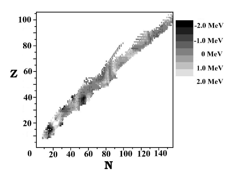
Figure 2: Distribution of $\Delta M(N,Z)$ in the $N-Z$ plane. The gray mass scale is given on the right.

Both the distribution of mass errors in the N-Z plane and the presence of the double peak in the error distribution suggest the presence of important correlations which are not taken into account in the FRDM mass formula. In the next sections these correlations are quantified and parametrized.

II Regularities in the mass errors

In order to visualize the oscillatory patterns suggested in Fig. 2, different cuts were performed along selected directions on the N-Z plane. Given the large number of chains which can be studied, we have selected those with the largest number of nuclei with measured mass. For each cut a Fourier analysis was performed, and the squared amplitudes are plotted as a function of the frequencies on the right hand side of each figure. The discrete Fourier transforms $F_{k}$ are calculated as

$$F_{k}={\frac{1}{\sqrt{N}}}\sum_{j}{\frac{\Delta M(j)}{\gamma}}\,\hbox{exp}\left({\frac{-2\pi ijk}{N}}\right),$$ (2)

where N is the number of mass differences $\Delta M$ in a given series. The parameter $\gamma$ makes $F_{k}$ dimensionless. Given that it only affects the global scale of the Fourier amplitudes, we made the simple selection $\gamma=1$ MeV. The Fourier amplitudes are plotted as functions of the frequency $f=k/N$. The presence of a few frequencies with notorious large components underlines the existence of an oscillatory behavior of the mass errors.

II.1 Fixed N or Z

We start our analysis for fixed N or Z, i.e. we selected different chains of isotopes and isotones. Those isotopic chains with 20 or more nuclei with measured masses are presented in Fig. 3 and 4. Until 1995, the element which had most isotopes with measured masses was Cs (Z=55) with 34.

Fig. 3 displays the mass errors for the isotope chains Z = 46 to 56, and their Fourier analysis, nearly all exhibiting a clear peak for the low frequency $f\approx 1/20=0.05$.

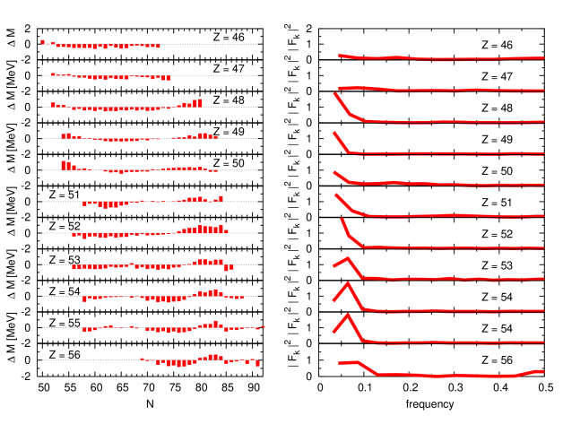
Figure 3: Mass errors in the isotope chains Z=46 to 56, and their Fourier analysis.

Fig. 4 displays the mass errors for the isotope chains Z = 30,36, 37, 38, 40, 87, 89, 91, and their Fourier analysis.

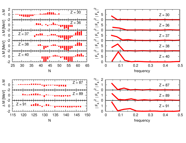
Figure 4: Mass errors in the isotope chains with Z = 30,36, 37, 38, 40, 87, 89, 91, and their Fourier analysis.

A similar analysis was performed for fixed N, i.e. isotonic chains, which have up to 30 nuclei with measured masses. Fig. 5 displays the mass errors for the isotone chains N=50 to 61, and their Fourier analysis.

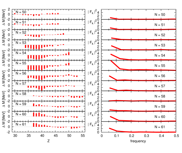
Figure 5: Mass errors in the isotone chains N=50 to 61, and their Fourier analysis.

Fig. 6 displays the mass errors for the isotone chains N=78 to 89, and their Fourier analysis.

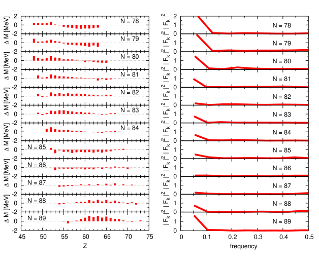
Figure 6: Mass errors in the isotone chains N=78 to 89, and their Fourier analysis.

Many isotopic chains exhibit similar oscillatory patterns in the mass errors. However, a Fourier decomposition for these cases is crude because there are only a few points, typically between 15 and 30, in each chain.

II.2 Fixed A or T_z

To map the mass error data in term of variables with the maximum possible number of nuclei along each chain, the following transformation is employed

$$\tilde{A}=Int[\sqrt{2}\,(N\,sin\theta\,+\,Z\,cos\theta)],~{}~{}~{}~{}\tilde{T}_{z}=Int[\sqrt{2}\,(N\,cos\theta\,-\,Z\,sin\theta)].$$ (3)

Both $\tilde{A}$ and $\tilde{T}_{z}$ are, by construction, integer numbers. To avoid introducing artificial noise, the data are softened by the interpolation of mass errors for unphysical values of $\tilde{T}_{z},\tilde{A}$, i.e. those with $\tilde{T}_{z}$ even and $\tilde{A}$ odd, or viceversa. This process is necessary to eliminate the large number of zeros which are induced by the transformation, which create artificial high frequency noise in the data.

Definition (3) has the advantage that, for $\theta=45^{\circ}$, $\tilde{A}=A,\tilde{T}_{z}=2T_{z}$. There are seven values of $T_{z}$ which have more than 40 nuclei with measured masses. They are $2T_{z}=5,6,7,8,16,17,18$. Their mass differences $\Delta M$ are plotted as a function of the mass number $A$ in the seven inserts shown in Fig. 7. The clustering of negative and positive errors is evident, again exhibiting the presence of residual correlations between the mass errors and the atomic and neutron numbers (Z, N), or, equivalently, with the isospin projection and the mass numbers.

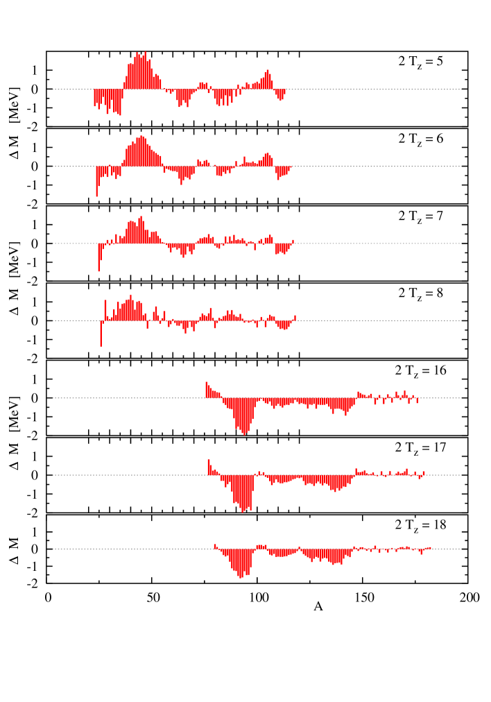
Figure 7: Mass differences as functions of $A$, for seven $T_{z}$ values.

The squared amplitudes of the Fourier transforms of the mass differences are shown in Fig. 8. For the first four isotopic chains ($2T_{z}=5,6,7,8$) there is a prominent peak at $f\approx 0.033$, i.e. a period $\Delta A\approx 30$, which is about one third the size of each set of nuclei. The remaining three chains exhibit also a peak at low frequencies, but lower and wider.

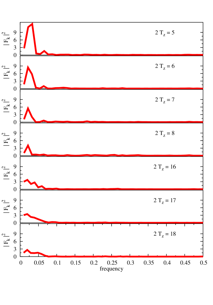
Figure 8: Squared amplitudes of the Fourier transforms of the mass differences, plotted as functions of $A$, for seven $T_{z}$ values.

In order to underline the relevance of the lower frequencies in the mass error distribution, in Fig. 9 the mass errors are plotted as a function of A, for $2T_{z}=6$ (left), and 8 (right), in the top panel. The middle panel exhibits the distribution obtained including only the three low frequencies: $f=0.011,0.022,0.033$. The second is the most important, with a period $\Delta A\approx 46$.

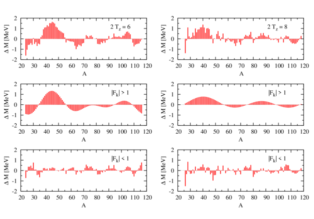
Figure 9: Mass differences as functions of $A$, for $2T_{z}=6$ (left), and 8 (right). The middle panels show the distribution for only the few frequencies with Fourier amplitudes larger than 1, the lower panels the distribution for all the remaining frequencies.

II.3 Rotated $\tilde{A}$ and $\tilde{T}_{z}$

We found that the best orientation, in order to have as many isotopes as possible with the same $\tilde{T}_{z}$, is $\theta=56^{\circ}$. With this transformation, there are 174 isotopes with $\tilde{T}_{z}=0$.

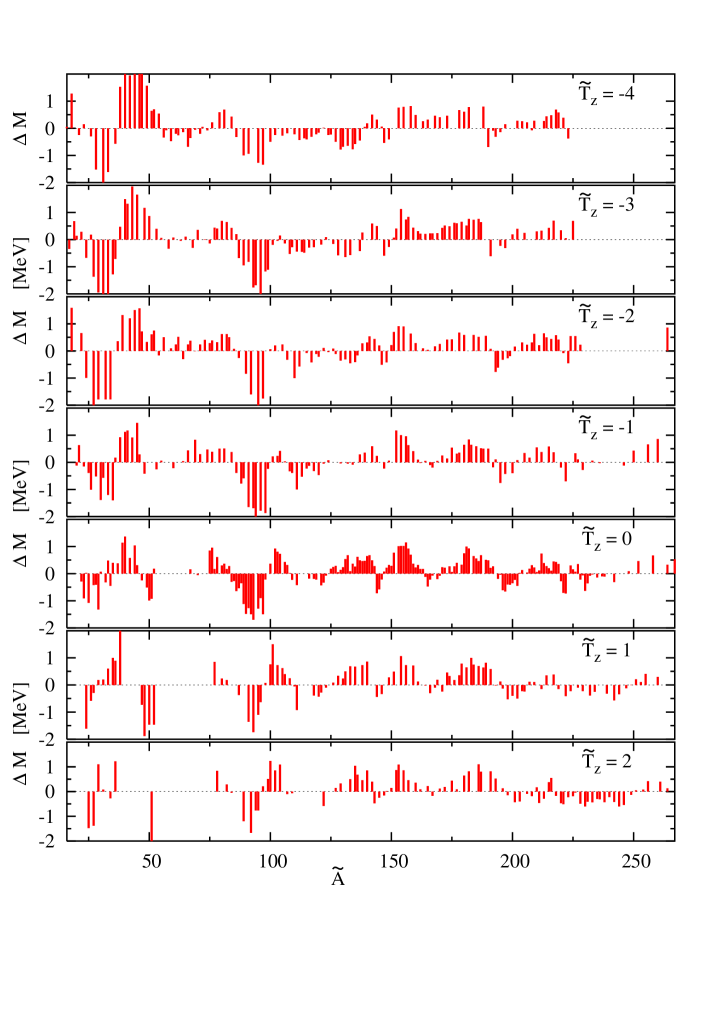
Figure 10: Mass differences as functions of $\tilde{A}$, for seven $\tilde{T}_{z}$ values.

Figure 10 displays the mass errors for 7 values of $\tilde{T}_{z}$, from $\tilde{T}_{z}=-4$ to 2. The regularities seen in Fig. 2 as regions with the same gray tone are seen here in the different plots, as groupings of nuclei with similar positive or negative mass differences, for the same $\tilde{A}$ region. Besides the two large groups with positive and negative mass errors below $\tilde{A}=50$, there are evident regions with negative errors close to $\tilde{A}=100$, and with positive mass differences for $150<\tilde{A}<200$.

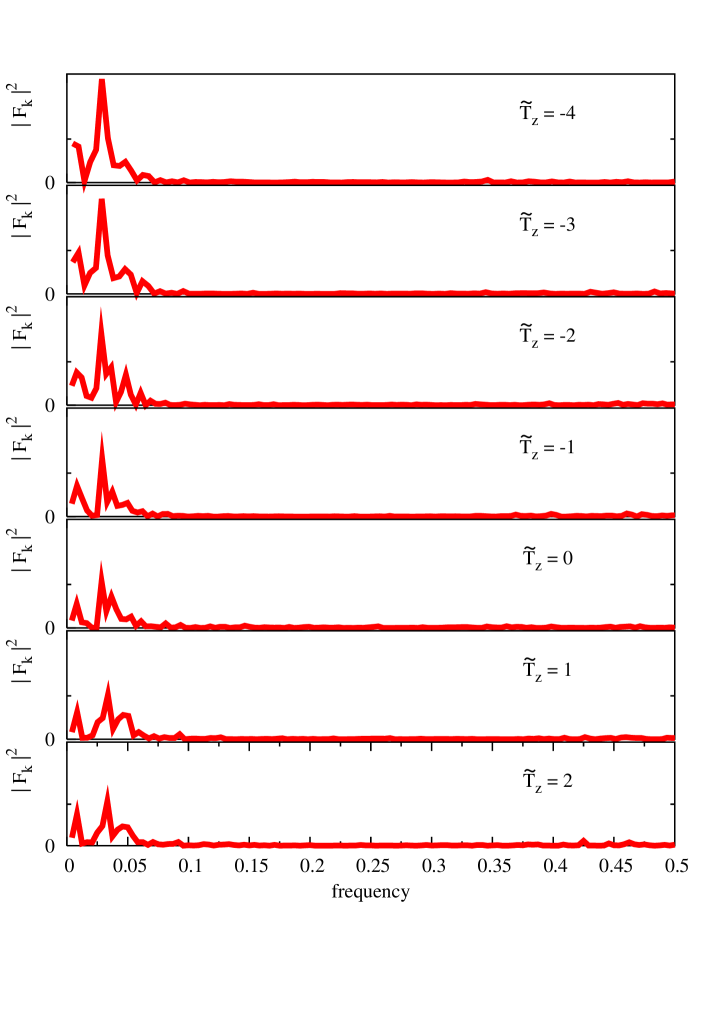
Figure 11: Squared amplitudes of the Fourier transforms of the mass differences, plotted as functions of the frequency, for seven $\tilde{T}_{z}$ values.

A Fourier analysis of the previous results is presented in Fig. 11. It is clear that for all the chains a few low frequencies again dominate the spectrum. In some chains there are also some higher frequencies which seem to be relevant, while for $\tilde{T}_{z}=0$ their contribution is small. These frequencies, close to $f=0.5$, are associated to oscillations with period 2, i.e. strong fluctuations between one nucleus and its closest neighbors.

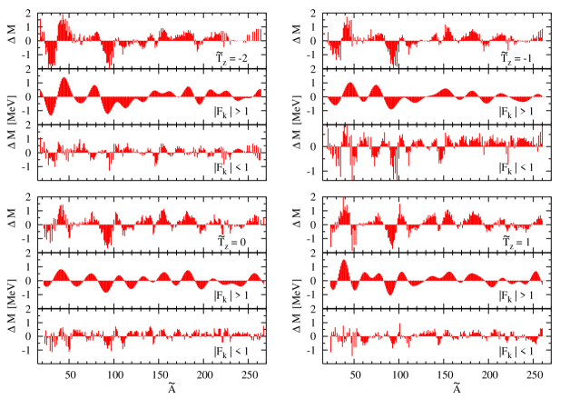
Figure 12: Mass differences as functions of $\tilde{A}$, for $\tilde{T}_{z}=-2$ (upper left), -1 (upper right), 0 (lower left) and 1 (lower right). The middle panels show the distribution for only the few frequencies with Fourier amplitudes larger than 1, the lower panels the distribution for all the remaining frequencies.

In Fig. 12 the contribution of very few frequencies to the mass differences, for the chains with $\tilde{T}_{z}=-2,-1,0$ and $1$ are presented. The upper panels show the full sequences of mass differences, the medium panels the contribution of the four frequencies with the largest amplitudes, and the lower panels the remaining mass errors. In all cases it is apparent that the regularities are quite significant, and that the substraction of these systematic errors would lead to important improvements in mass calculations.

II.4 Bustrofedon: all data aligned

Plotting the mass differences for different Z, Fig. 13 top, and for different N, Fig. 13 bottom, is very common in mass calculations. Both plots exhibit some degree of structure. In this way we obtain a plot of mass differences as a function of Z, with all the isotopes plotted along the same vertical line, see Fig. 13. The difficulty in quantifying these regularities lies in the simple fact that the are many nuclei with a given N or Z. For this reason in the previous subsections we have analyzed the data using different cuts.

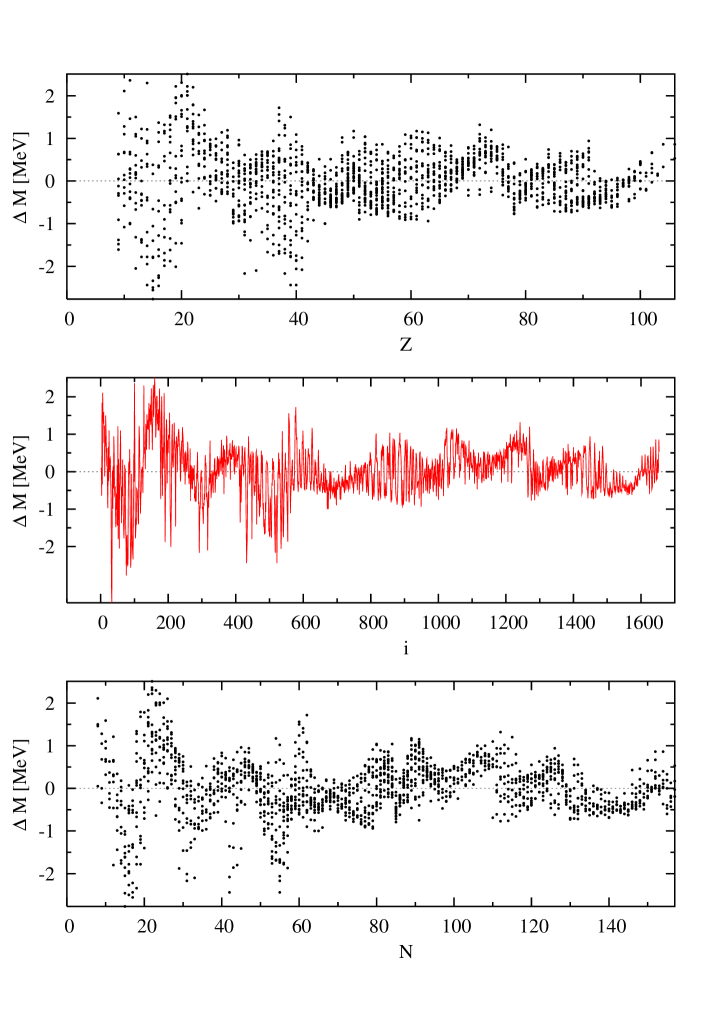
Figure 13: Mass differences plotted as function of Z (top), N (bottom), and of an ordered list (middle)

Another way to organize the FRDM mass errors for the 1654 nuclei with measured masses is to order them in a single list, numbered in increasing order. To avoid jumps, we have ordered the isotopes along a $\beta{}o\upsilon\tau\rho{}o\phi\eta\delta\acute{o}\nu$ (bustrofedon) line, which literally means ”in the way the ox ploughs”. Nuclei were ordered in increasing mass order. For a given even A, they were accommodated following the increase in N-Z, and those nuclei with odd A starting from the largest value of N-Z, and going on in decreasing order. The middle panel exhibits the same mass differences plotted against the order number, from 1 to 1654. It provides a univalued function, whose Fourier transform can be calculated. The squared amplitudes are presented in Fig. 14.

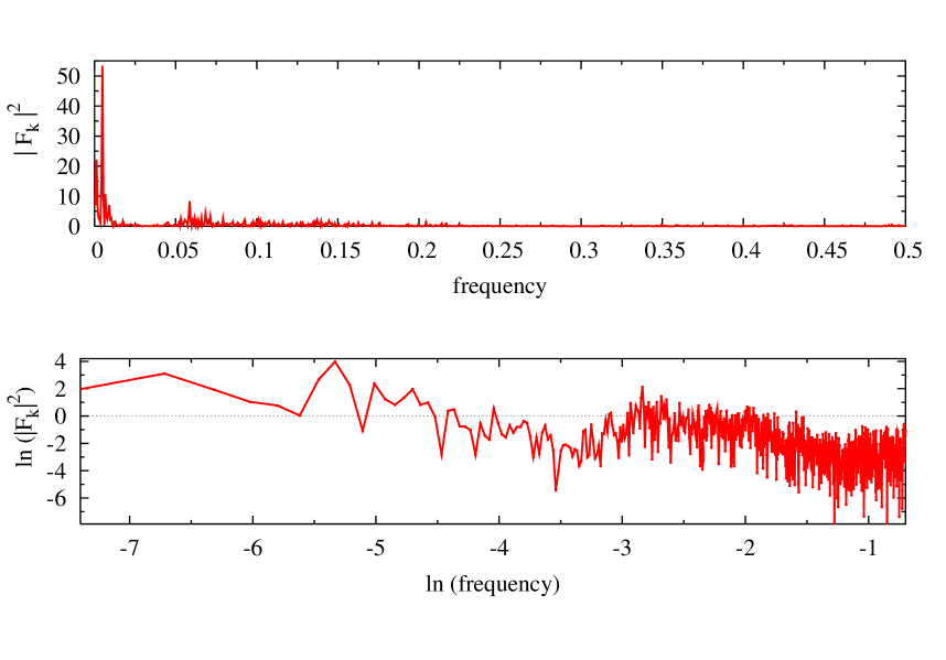
Figure 14: Squared amplitudes of the Fourier transforms of the mass differences, plotted as functions of the frequency (top). Power spectrum: natural logarithm of squared amplitudes of the Fourier transforms of the mass differences (bottom).

As it was the case for the cuts for given N, Z, A ot T_z, the fully ordered data Fourier amplitudes are completely dominated by a few low frequencies. It is also remarkable that for ln(f) $>$ -3 the frequency distribution clearly resembles a power law.

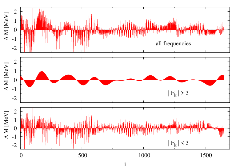
Figure 15: Mass differences plotted as an ordered list (top). Mass error function recovered when only those Fourier amplitudes larger than 3 are considered (middle) , and the mass error function which remains when the larger Fourier amplitudes are removed (bottom).

Removing the five frequencies with the largest Fourier components ($|F_{k}|>3$) generates a noisier pattern. Figure 15 shows the mass differences plotted as function of the order index, and the results of leaving only the frequencies with amplitudes $|F_{k}|$ larger (or smaller) than 3. There only five frequencies with Fourier amplitudes whose absolute value is larger than 3. From them the dominant frequency is the one with period $\Delta i=207$. The regular pattern generated by these five frequencies in displayed in the middle panel of Fig. 15. The remnant, shown in the bottom panel, is clearly closer to white noise, while some bumps remain.

From the analysis presented in this section, we can conclude that there are conspicuous correlations in the FRDM mass differences, whose periodic character is clearly exhibited by the Fourier analysis of different cuts. It is worthwhile to study the slope of the squared amplitudes against the frequencies (i.e. the power spectra) in a log-log plot, which in a random matrix context was found to offer a signature of quantum chaos Rel02 . This is of great interest in itself and will be analyzed in a separate publication Vel03b .

III Removing the regularities

Having established that there are patent regularities in the differences between the masses calculated using the FRDM Moll95 and the measured ones, we will proceed to eliminate them in a simple way, by removing the two frequencies which contribute the most to the mass errors as functions of N and Z. We introduce an amplitude and a phase for each frequency, having a total of six parameters for protons and six for neutrons. The functions which minimize the errors separately for protons and neutrons are:

$$\Delta_{1}(N)=.30\,\,\mbox{\rm sin}(2\pi.012N+.284)+.20\,\,\mbox{\rm sin}(2\pi.047N+1.06)$$ (4)

$$\Delta_{1}(Z)=.23\,\,\mbox{\rm sin}(2\pi.020Z-0.83)+.10\,\,\mbox{\rm sin}(2\pi.053Z+3.74)$$ (5)

In a fit including all nuclei, we found

$$\Delta_{2}(N)=.21\,\,\mbox{\rm sin}(2\pi.011N+0.86)+.34\,\,\mbox{\rm sin}(2\pi.049N+0.17)$$

$$\Delta_{2}(Z)=.14\,\,\mbox{\rm sin}(2\pi.025Z-0.74)-.19\,\,\mbox{\rm sin}(2\pi.075Z-5.53)$$

$$\Delta_{2}(N,Z)=\Delta_{2}(N)+\Delta_{2}(Z),$$ (6)

while including only nuclei with A $\geq$ 65 the best fit is

$$\Delta_{3}(N)=.65\,\,\mbox{\rm sin}(2\pi.009N+2.03)+.19\,\,\mbox{\rm sin}(2\pi.047N+1.00)$$

$$\Delta_{3}(Z)=2.90\,\,\mbox{\rm sin}(2\pi.018Z-3.51)+2.61\,\,\mbox{\rm sin}(2\pi.019Z-0.74)$$

$$\Delta_{3}(N,Z)=\Delta_{3}(N)+\Delta_{3}(Z).$$ (7)

The $\Delta_{1}$ are functions only of N or Z, and were adjusted using six parameters, optimized for the 1350 nuclei with A $\geq$ 65. $\Delta_{2}$ and $\Delta_{3}$ are obtained by including at the same time the corrections in Z and N, for all the nuclei in the first case, and for those with A $\geq$ 65 in the second. The fitted frequencies are all between 0.01 and 0.05, in agreement with the dominant Fourier frequencies found in the previous section.

The effect of removing these sinusoidal components as functions of N and Z is shown in Fig. 16, for those nuclei with masses larger than 65.

Figure 16: Mass differences plotted as function of Z (left) and N (right), for A $\geq$ 65. The upper panels exhibit the FRDM results, the intermediate ones the sinusoidal corrections, and the lower panels the corrected mass differences.

While the regular pattern is more apparent as a function of N, on the right hand side panels, in both cases the ‘corrected’ masses are more compact and compressed at smaller errors.

Obtaining a better fit of the known nuclear masses by the inclusion of six or twelve extra variables is by no means surprising. However, the use of sinusoidal functions of N and Z is strongly motivated by the data themselves. The fit does not only reduce the overall error, but makes the double peak in the error distribution disappear, as shown in Fig. 17 for all the nuclei, and in Fig. 18 for nuclei with A $\geq$ 65.

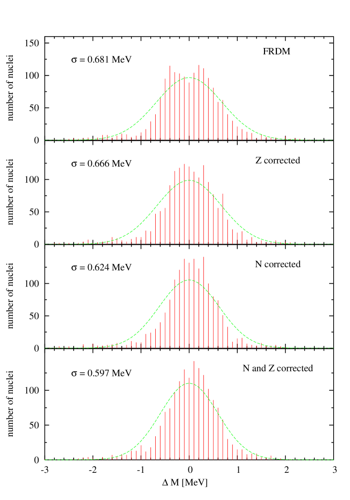
Figure 17: Distribution of FRDM mass differences corrected with a sinusoidal function of Z, of N, and of Z and N.

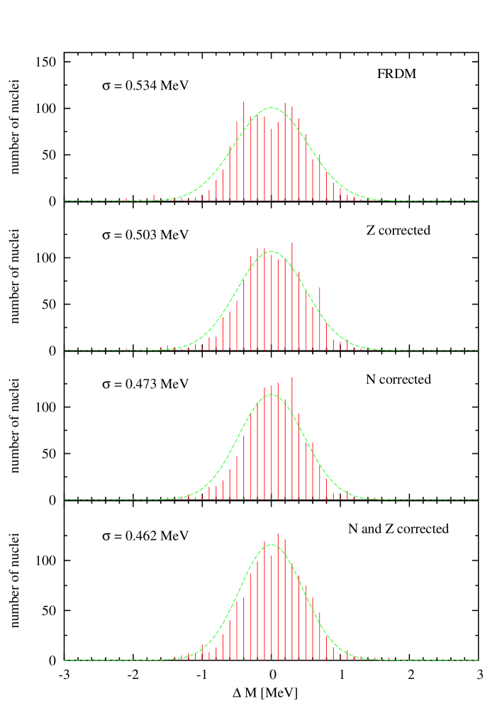
Figure 18: Distribution of FRDM mass differences for A $\geq$ 65, corrected with a sinusoidal function of Z, of N, and of Z and N.

In both figures the error width reduction is evident, as well as the concentration of the mass differences around zero, with a single peak. The continuous curve represents a Gaussian curve with the same width and normalization. After removing the oscillatory components, the r.m.s. mass errors is reduced from 0.681 MeV to 0.597 MeV for all nuclei, and from 0.534 MeV to 0.462 MeV for nuclei with A $\geq$ 65.

IV Final remarks

In the present study we have shown that the differences between the masses calculated using the FRDM of Möller at al Moll95 and the measured ones have a well defined oscillatory component as function of N and Z, which can be removed with an appropriate fit, significantly reducing the error width, and concentrating the error distribution on a single peak around zero.

The remaining correlations can only originate in the microscopic terms in the mass formula, which in the FRDM are evaluated using the Strutinsky method Bra72 . Having shown that these correlations have a simple and clear dependence in the proton and neutron numbers, we are studying the possible removal of these effects by a refinement of the Strutinsky method, whose results will be reported elsewhere Vel03b .

References

- (1) C.E. Rolfs and W.S. Rodney, Cauldrons in the Cosmos, University of Chicago Press (1988).
- (2) P. Möller, J.R. Nix, W.D. Myers, W.J. Swiatecki, At. Data Nucl. Data Tables 59, 185 (1995).
- (3) J. Duflo, Nucl. Phys. A 576, 29 (1994); J. Duflo and A. P. Zuker, Phys. Rev. C 52, R23 (1995).
- (4) S. Goriely, F. Tondeur, and J.M. Pearson, Atom. Data Nucl. Data Tables 77, 311 (2001).
- (5) Víctor Velázquez, Alejandro Frank, and Jorge G. Hirsch, Proc. of the workshop Computational and Group Theoretical Methods in Nuclear Physics, Playa del Carmen, Mexico, February 18 - 22, 2003, World Scientific, Singapore, in press.
- (6) A. Relaño, J.M.G. Gómez, R.A. Molina, J. Retamosa and E. Faleiro, Phys. Rev. Lett. 89 (2002) 244102.
- (7) M. Brack, Jens Damgaard, A.S. Jensen, H.C. Pauli, V.M. Strutinsky, C.Y. Wong, Rev. Mod. Phys. 44 (1972) 320; V.M. Strutinsky and F.A. Ivanjuk, Nucl. Phys. A 255 (1975) 405.
- (8) Víctor Velázquez, Alejandro Frank, and Jorge G. Hirsch, in preparation.