Hydrodynamical instabilities in an expanding quark gluon plasma

Abstract

We study the mechanism responsible for the onset of instabilities in a chiral phase transition at nonzero temperature and baryon chemical potential. As a low-energy effective model, we consider an expanding relativistic plasma of quarks coupled to a chiral field, and obtain a phenomenological chiral hydrodynamics from a variational principle. Studying the dispersion relation for small fluctuations around equilibrium, we identify the role played by chiral waves and pressure waves in the generation of instabilities. We show that pressure modes become unstable earlier than chiral modes.

I Introduction

It is commonly believed that QCD at very high temperatures and/or densities allows for a new phase of strongly interacting matter, the quark-gluon plasma (QGP). Compelling lattice QCD results point in that direction Karsch:2001vs , and experiments in ultra-relativistic heavy-ion collisions rhic under way at BNL-RHIC QM2004 and planned for CERN-LHC attempt to glimpse at this elusive state of matter that was presumably present in the early universe cosmo .

Depending on the nature of the QCD phase transition, the hadronization process of the expanding QGP generated in a high-energy heavy-ion collision may proceed in a number of different ways review . In the analysis of phase conversion of strongly interacting matter from a chirally symmetric to a chirally broken state in the phase diagram of QCD, a mechanism of supercooling is usually implied QM2004 ; cosmo . The kinetics of domain formation and growth can then be described by the the mechanisms of nucleation or spinodal decomposition, depending on the degree of supercooling review . An expanding plasma will probe, in principle, different temperatures and experiment both mechanisms. In the case of the early universe, it is well known that the time scales for the expansion during the QCD transition are so slow that phase conversion is driven by the nucleation of bubbles of true vacuum inside the metastable phase, as the universe reaches temperatures below a critical value cosmo . On the other hand, the QGP presumably created in experiments in ultra-relativistic heavy-ion collisions expands at a pace several orders of magnitude faster than the primordial universe QM2004 ; rhic , and might simply bypass nucleation, entering the domain of spinodal decomposition sudden ; Scavenius:1999zc ; Scavenius:2001bb ; Shukla:2001xv ; explosive ; polyakov-explosive . Some results from CERN-SPS and BNL-RHIC suggest what has been called sudden hadronization sudden or explosive behavior polyakov-explosive ; explosive . From the theoretical side, this phenomenon was recently associated with rapid changes in the effective potential of QCD near the critical temperature, such as predicted, for instance, by the Polyakov loop model polyakov ; polyakov-explosive , followed by spinodal decomposition review ; explosive . Clearly, an understanding of the interplay between the typical space and time scales of the expanding plasma is welcome. Some attempts in this direction can be found in Refs. quarks-chiral ; ove ; Scavenius:1999zc ; Scavenius:2001bb ; paech ; bravina ; Shukla:2001xv ; finite1 ; finite2 ; randrup ; FK .

In this paper, we discuss the mechanism responsible for the onset of instabilities in an expanding plasma. As a phenomenological model to mimic the case of the QGP, we use a relativistic plasma of quarks coupled to a chiral field. Although we derive a phenomenological chiral hydrodynamics from a variational principle, we do not focus on the numerical solution of the resulting hydrodynamic transport equations. Rather, we consider the role played by chiral waves and pressure waves in the generation of unstable modes. We show that mechanical instabilities set in earlier than one would expect from the analysis of the thermodynamic potential decoupled from hydrodynamical modes. Therefore, the spinodal lines are shifted from the values one obtains studying only the chiral degrees of freedom, modifying the phase diagram.

It has been argued critical-point ; critical2 ; Scavenius:2000qd that the first-order transition line which starts at the $T=0$ axis of the baryon chemical potential ($\mu$) vs. temperature ($T$) phase diagram for QCD should come to an end at a critical point $(\mu_{E},T_{E})$. Beyond this endpoint, for $0<\mu<\mu_{E}$, the QCD transition should become a smooth crossover, where spinodal instabilities do not occur. Results from lattice simulations at finite $\mu$ also point in this direction fodor ; allton . Here, we consider two illustrative scenarios for the temperature ($T$) vs. baryon chemical potential ($\mu$) phase diagram in which a first order line starts at a point $(\mu,T)=(\mu_{c},0)$ and ends in a critical point, $(\mu_{E},T_{E})$, with $\mu_{E}<\mu_{c}$, beyond which, for $0<\mu<\mu_{E}$, the phase transition becomes a smooth crossover.

To model the mechanism of chiral symmetry breaking present in QCD, we adopt a simple low-energy effective chiral model: the linear $\sigma$-model coupled to quarks gellmann , which in turn comprise the hydrodynamic degrees of freedom of the system. Similar approaches, relying on low-energy effective models for QCD and making use of a number of techniques to treat the expanding plasma, can be found in the literature quarks-chiral ; ove ; Scavenius:1999zc ; Scavenius:2001bb ; paech . The gas of quarks provides a thermal bath in which the long-wavelength modes of the chiral field evolve. The latter plays the role of an order parameter in a Landau-Ginzburg approach to the description of the chiral phase transition Scavenius:2001bb ; paech .

The paper is organized as follows. In section II, we present our effective field theory model. In section III, we derive what we call phenomenological chiral hydrodynamics from a variational formulation of relativistic hydrodynamics. In section IV, we study the onset of instabilities. In section V, we discuss our results.

II The effective model

Let us consider a chiral field $\phi=(\sigma,\vec{\pi})$, where $\sigma$ is a scalar field and $\pi^{i}$ are pseudoscalar fields playing the role of the pions, coupled to two flavors of quarks according to the Lagrangian:

$$\mathcal{L}=\overline{q}[i\gamma^{\mu}\partial_{\mu}+\mu_{q}\gamma^{0}-W(\phi)]q+\frac{1}{2}\partial_{\mu}\phi\partial^{\mu}\phi-V(\phi)\;.$$ (1)

Here $q$ is the constituent-quark field $q=(u,d)$ and $\mu_{q}=\mu/3$ is the quark chemical potential. The interaction between the quarks and the chiral field is given by

$$W(\phi)=g\left(\sigma+i\gamma_{5}\vec{\tau}\cdot\vec{\pi}\right)\;,$$ (2)

and

$$V(\phi)=\frac{\lambda^{2}}{4}\left(\sigma^{2}+\vec{\pi}^{2}-v^{2}\right)^{2}-h_{q}\sigma$$ (3)

is the self-interaction potential for $\phi$. The parameters above are chosen such that chiral $SU_{L}(2)\otimes SU_{R}(2)$ symmetry is spontaneously broken in the vacuum. The vacuum expectation values of the condensates are $\langle\sigma\rangle=\mathit{f}_{\pi}$ and $\langle\vec{\pi}\rangle=0$, where $\mathit{f}_{\pi}=93$ MeV is the pion decay constant. The explicit symmetry breaking term is due to the finite current-quark masses and is determined by the PCAC relation, giving $h_{q}=f_{\pi}m_{\pi}^{2}$, where $m_{\pi}=138$ MeV is the pion mass. This yields $v^{2}=f^{2}_{\pi}-{m^{2}_{\pi}}/{\lambda^{2}}$. The value of $\lambda^{2}=20$ leads to a $\sigma$-mass, $m^{2}_{\sigma}=2\lambda^{2}f^{2}_{\pi}+m^{2}_{\pi}$, equal to 600 MeV. In mean field theory, the purely bosonic part of this Lagrangian exhibits a second-order phase transition Pisarski:1984ms at $T_{c}=\sqrt{2}v$ if the explicit symmetry breaking term, $h_{q}$, is dropped. For $h_{q}\neq 0$, the transition becomes a smooth crossover from the restored to broken symmetry phases. For $g>0$, the finite-temperature one-loop effective potential also includes a contribution from the quark fermionic determinant Scavenius:2001bb ; paech .

In what follows, we treat the gas of quarks as a heat bath for the chiral field, with temperature $T$ and baryon-chemical potential $\mu$. Then, one can integrate over the fermionic degrees of freedom, obtaining an effective theory for the chiral field $\phi$. To compute thermodynamic quantities, one needs the partition function

$${\cal Z}=\int[{\cal D}\phi][{\cal D}q][{\cal D}\overline{q}]e^{-\int_{0}^{1/T}d\tau\int_{\cal V}d^{3}x{\cal L}_{E}}\quad,$$ (4)

where ${\cal L}_{E}$ is the Euclidean Lagrangian and ${\cal V}$ is the (infinite) volume of the plasma. Integrating over the fermions and using a classical approximation for the chiral field, we can write the thermodynamic potential as

$$\Omega(T,\mu,\phi)=V(\phi)-\frac{T}{\mathcal{V}}\ln\det\{[G_{E}^{-1}+W(\phi)]/T\}\;,$$ (5)

where $G_{E}$ is the fermionic Euclidean propagator satisfying

$$\left[\gamma^{0}\partial_{\tau}+i\vec{\gamma}\cdot\nabla-\mu\gamma^{0}\right]G_{E}(\tau,\vec{x};\tau^{\prime},\vec{x}^{\prime})=\delta^{(4)}(x-x^{\prime})\;.$$ (6)

From the thermodynamic potential, (5), one can obtain all the thermodynamic quantities of interest. The fermionic determinant that results from the functional integration over the quark fields can be calculated to one-loop order in the standard fashion Scavenius:2000qd ; kapusta-book . The effective Lagrangian for the chiral field, $\phi$, in the presence of the quark thermal bath is then

$$\mathcal{L}_{eff}^{(\phi)}=\frac{1}{2}\partial_{\mu}\phi\partial^{\mu}\phi-\Omega(T,\mu,\phi).$$ (7)

III Chiral hydrodynamics

Given the thermodynamic potential, one can derive the total pressure and energy density, and obtain the conserved energy-momentum tensor, $\mathcal{T}^{\mu\nu}$, for an expanding quark perfect fluid by using standard methods of thermal field theory (see, for instance, Ref. paech ). We prefer, instead, adopting an alternative approach to obtain the hydrodynamic equations for our system: the variational formulation Bailyn ; variational . This approach provides a natural and unified way of merging chiral and fluid dynamics once the action of the system is specified. For a different treatment of the hydrodynamics of nuclear matter in the chiral limit, see son .

The variational formulation of relativistic hydrodynamics has been recently applied to several physical systems, especially in the realms of astrophysics and condensed matter. In the former it has been used, for instance, to incorporate the effects of local turbulent motion in supernova explosion mechanisms, and can prove to be useful in the analysis of the relativistic motion of blast waves in models for gamma-ray bursts astro . In soft condensed matter, it has been used to study the bubble dynamics in sonoluminescence experiments, in particular in deriving the relativistic generalization of the Rayleigh-Plesset equation cond-mat . In this section, we briefly review how to obtain the usual equations of relativistic hydrodynamics within this framework, and derive in detail the case in which we have a chiral field coupled to an expanding quark fluid.

We describe the state of the fluid in terms of the four-velocity $u^{\mu}(x)$, the proper baryon density, $n(x)$, and the proper entropy density, $s(x)$. In what follows we assume that $n$ and $s$ are conserved, i.e.:

$$\partial_{\mu}(nu^{\mu}) = 0\;,$$

$$\partial_{\mu}(su^{\mu}) = 0\;.$$ (8)

The action that yields the hydrodynamic equations is given by Bailyn ; variational

$$S^{(fluid)}\equiv\int d^{4}x\left[-\epsilon(n,s)\right]\;,$$ (9)

where $\epsilon(n,s)$ is the proper energy density, from which temperature and chemical potential are obtained via the usual thermodynamic relations, $T=\partial\epsilon(n,s)/\partial s$ and $\mu=\partial\epsilon(n,s)/\partial n$. The equation for the hydrodynamic motion of the fluid is obtained by imposing the variational principle with respect to $n$, $s$ and $u^{\mu}$, under the constraints (8) and the normalization condition

$$u^{\mu}u_{\mu}=1\;.$$ (10)

These constraints can be incorporated in the variational principle in terms of Lagrangian multipliers, $\lambda(x)$, $\zeta(x)$ and $w(x)$, so that one imposes:

$$\delta\int d^{4}x\left[\right. - \epsilon(n,s)+\lambda\partial_{\mu}(nu^{\mu})+\zeta\partial_{\mu}(su^{\mu})$$ (11)

$$+ \left.\frac{1}{2}w\left(u^{\mu}u_{\mu}-1\right)\right]=0,$$

Equivalently, the fluid dynamics is given by the effective Lagrangian, $\mathcal{L}_{eff}^{\left(fluid\right)}=\mathcal{L}_{eff}^{\left(fluid\right)}\left(n,s,u^{\mu},\lambda,\zeta,w\right)$,

$$\mathcal{L}_{eff}^{\left(fluid\right)} = -\epsilon(n,s)-nu^{\mu}\partial_{\mu}\lambda$$ (12)

$$- su^{\mu}\partial_{\mu}\zeta+\frac{1}{2}w\left(u^{\mu}u_{\mu}-1\right)\;.$$

Now the variables $n$, $s$, $u^{\mu}$, $\lambda$, $\zeta$, and $w$ are independent.

Variations with respect to $n$, $s$ and $u^{\mu}$ yield

$$-\mu-u^{\mu}\partial_{\mu}\lambda = 0\;,$$

$$-T-u^{\mu}\partial_{\mu}\zeta = 0\;,$$

$$-n\partial_{\mu}\lambda-s\partial_{\mu}\zeta+wu_{\mu} = 0\;,$$ (13)

while variations with respect to $\lambda$, $\zeta$ and $w$ give simply the constraints (8) and (10). From (10) and (13), one obtains

$$w = n\mu+Ts$$ (14)

$$= \varepsilon+p\;,$$

where $p$ is the pressure, and identifies $w$ as the enthalpy density. Using the Gibbs-Duhem relation, $dp=sdT+nd\mu$, and the property $u^{\nu}(\partial_{\mu}u_{\nu})=0$, it is straightforward to obtain

$$\partial^{\nu}\left(wu_{\mu}u_{\nu}\right) = n\partial_{\mu}\mu+s\partial_{\mu}T+\left(\partial_{\mu}u_{\nu}\right)\xi u^{\nu}$$ (15)

$$= \partial_{\mu}p+u^{\nu}\left(\partial_{\mu}u_{\nu}\right)\xi$$

$$= \partial_{\mu}p\;,$$

which can be rewritten in the standard form

$$\partial^{\nu}T_{\mu\nu}=0,$$ (16)

where

$$T_{\mu\nu} = wu_{\mu}u_{\nu}-g_{\mu\nu}p$$ (17)

$$= \left(p+\varepsilon\right)u_{\mu}u_{\nu}-g_{\mu\nu}p$$

is the usual energy-momentum tensor of the fluid.

It is important to notice that the effective Lagrangian, (12), evaluated in the proper comoving frame of the fluid,

$$\mathcal{L}_{eff}^{\left(fluid\right)}=-\epsilon(n,s)+\mu n+Ts=p\;,$$ (18)

is nothing but minus the thermodynamic potential of the system. This fact will be useful to couple the chiral degrees of freedom to the quark fluid motion.

The procedure outlined above for the derivation of relativistic hydrodynamics presents a number of nice features. First, it can be easily generalized to include other degrees of freedom such as the chiral field. Secondly, although we have implicitly used a Minkowski metric, the generalization to the case of curved space-times is straightforward. This will be discussed later, when we consider applications to cosmology. Furthermore, from a practical point of view, once the variational approach is established one can use this method to obtain the optimal parameters for a given family of trial solutions.

Let us now describe how to couple a chiral field to the fluid within the framework of the variational principle. The effective Lagrangian for the chiral field, (7), should be interpreted as the proper value of the Lagrangian where the thermalized quark fluid is at rest. Therefore, Eq. (18) suggests that the part corresponding to the quark pressure should be replaced by expression (12) in order to reconstruct the fluid motion of thermalized quarks. Apart from the constraints, we have the following action for the coupled system of the chiral field, $\phi$, and the thermalized quark fluid motion:

$$S^{\left(\phi+fluid\right)}=\int d^{4}x\left\{\frac{1}{2}(\partial_{\mu}\phi)(\partial^{\mu}\phi)-\epsilon(n,s,\phi)\right\}\;.$$ (19)

Here, the energy density, $\epsilon$, is related to the thermodynamic potential, $\Omega$, through the Legendre transformation $\epsilon=\Omega+Ts+\mu n$. Since $\Omega=-p$, this is nothing but the general thermodynamic relation $\epsilon=-p+Ts+\mu n$. Notice that now the energy density depends on the field variable $\phi$ through $\Omega=\Omega\left(T,\mu,\phi\right)$ and, correspondingly, the second thermodynamic law should read

$$d\epsilon=Tds+\mu dn+Rd\phi\;.$$ (20)

The corresponding Gibbs-Duhem relation becomes

$$dp=sdT+nd\mu-Rd\phi\;,$$ (21)

where we have defined a new quantity $R$ (with four components $R_{i}=\partial\Omega/\partial\phi_{i}$):

$$R \equiv \left(\frac{\partial\epsilon(n,s,\phi)}{\partial\phi}\right)_{n,s}$$ (22)

$$= \left(\frac{\partial\Omega(T,\mu,\phi)}{\partial\phi}\right)_{T,\mu}\;.$$

The second line corresponds to Maxwell’s relation and comes from Eq. (21). $R$ can be written as

$$R=\frac{\partial V(\phi)}{\partial\phi}+g\phi\rho(T,\mu,\phi)\;,$$ (23)

where

$$\rho=\nu_{q}\int\frac{d^{3}k}{(2\pi)^{3}}\frac{1/E_{k}(\phi)}{e^{[E_{k}(\phi)-\mu_{q}]/T}+1}+(\mu_{q}\rightarrow-\mu_{q})$$ (24)

is a scalar density for quarks. Here $\nu_{q}=12$ stands for the color-spin-isospin degeneracy of the quarks, $E_{k}(\phi)=(\vec{k}^{2}+m_{q}^{2}(\phi))^{1/2}$, and $m_{q}(\phi)=(g^{2}\phi^{2})^{1/2}=g(\sigma^{2}+\vec{\pi}^{2})^{1/2}$ plays the role of an effective mass for the quarks.

Thus, our coupled system is described by an effective Lagrangian

$$\mathcal{L}_{eff}^{\left(\phi+fluid\right)} = \frac{1}{2}(\partial_{\mu}\phi)(\partial^{\mu}\phi)-\epsilon(n,s,\phi)-nu^{\mu}\partial_{\mu}\lambda$$ (25)

$$- su^{\mu}\partial_{\mu}\zeta+\frac{1}{2}w\left(u^{\mu}u_{\mu}-1\right)\;.$$

The variation with respect to $\phi$ gives the equation of motion for the chiral field,

$$\Box\phi=-R\;$$ (26)

The variation procedures with respect to the fluid variables are almost exactly the same as before, except for the use of the new Gibbs-Duhem relation, (21). Thus, Eq. (15) is modified to

$$\partial^{\nu}\left(wu_{\mu}u_{\nu}\right)=\partial_{\mu}p+R\partial_{\mu}\phi,$$ (27)

or, in the standard form,

$$\partial^{\nu}T_{\nu\mu}=R\partial_{\mu}\phi\;,$$ (28)

where $T_{\mu\nu}$ is given by Eq. (17) and is not the total energy momentum tensor of the system, $\mathcal{T}^{\mu\nu}=T^{\mu\nu}-\frac{1}{2}\partial_{\alpha}\phi\partial^{\alpha}\phi g^{\mu\nu}+\partial^{\mu}\phi\partial^{\nu}\phi$, which is of course conserved.

Note that Eq. (28) contains terms from the pure contribution of the field $\phi,$ such as $V\left(\phi\right)$ and $\partial V/\partial\phi$, both in $T_{\mu\nu}$ and in $R$. However, as we can see from the equivalent equation, (27), some of these terms cancel out. To see more clearly the coupling between the fluid equation and the chiral field $\phi$, it may be convenient to identify the fluid contribution of the pressure as

$$p^{\left(fluid\right)}=\frac{T}{\mathcal{V}}\ln\det[(G_{E}^{-1}+W(\phi))/T]\;,$$ (29)

and the energy-momentum tensor of the fluid,

$$T_{\mu\nu}^{\left(fluid\right)}=wu_{\mu}u_{\nu}-p^{\left(fluid\right)}g_{\mu\nu}.$$ (30)

Then the hydrodynamical motion is written as

$$\partial^{\mu}T_{\mu\nu}^{\left(fluid\right)}-\rho(\phi)m_{q}\partial_{\nu}m_{q}(\phi)=0\;.$$ (31)

IV Stability analysis

A numerical analysis of the system of differential equations consisting of (31) and the equations of motion for $\sigma$ and $\vec{\pi}$ was performed, for instance, in Refs. ove ; paech . Here, we refrain from this approach and, instead, consider the behavior of small oscillations around equilibrium to study the onset of instabilities.

In what follows, we expand around equilibrium keeping terms up to first order in the perturbation, i.e.:

$$n(x) = n_{eq}+n_{1}(x)\;,$$

$$s(x) = s_{eq}+s_{1}(x)\;,$$

$$\phi(x) = \phi_{eq}+\phi_{1}(x)\;,$$

$$u^{\nu}(x) = u^{\nu}_{eq}+u^{\nu}_{1}(x)\;.$$ (32)

Since the normalization of the four-velocity implies $u_{1}^{\nu}=(0,\vec{v}_{1})$, and $R_{eq}=0$, the conservation laws (8) yield

$$\frac{\partial n_{1}}{\partial t}+n_{eq}\nabla\cdot\vec{v}_{1}=0\;,$$

$$\frac{\partial s_{1}}{\partial t}+s_{eq}\nabla\cdot\vec{v}_{1}=0\;,$$ (33)

and the chiral field equation of motion becomes

$$(\Box+m^{2}_{\phi})\phi=-\left(\frac{\partial R}{\partial n}\right)_{eq}n_{1}-\left(\frac{\partial R}{\partial s}\right)_{eq}s_{1}\;,$$ (34)

where we have defined the (diagonal) chiral mass matrix

$$m^{2}_{\phi}\equiv\left[\frac{\partial^{2}\epsilon(n,s,\phi)}{\partial\phi^{2}}\right]_{eq}\;.$$ (35)

The time component of Euler’s equation, (27), is automatically satisfied given the conservation laws above, and its spatial components yield

$$w_{eq}\frac{\partial\vec{v}_{1}}{\partial t}=-\nabla p_{1}\;.$$ (36)

For plane waves of the form $\psi_{1}(x)=\tilde{\psi}_{1}e^{-iKx}$, where $K^{\mu}=(\omega,\vec{k})$ and $\psi_{1}$ stands for $n_{1}$, $s_{1}$, $\phi_{1}$ or $\vec{v}_{1}$, we can rewrite the wave equation, (34), and the spatial component of Euler’s equation, (36), as (dropping the tildes)

$$(\omega^{2}-{k}^{2}-m_{\pi}^{2})~{}\vec{\pi}_{1} = 0\;,$$ (37)

$$(\omega^{2}-{k}^{2}-m_{\sigma}^{2})~{}{\sigma}_{1} = \frac{k}{\omega}w_{eq}R^{\prime}{v}_{1}\;,$$ (38)

$$(\omega^{2}-p^{\prime}{k}^{2})~{}{v}_{1} = \omega kR^{\prime}{\sigma}_{1}\;,$$ (39)

where we have defined

$$p^{\prime}\equiv\left[\frac{\partial p(\epsilon,n/s,\phi)}{\partial\epsilon}\right]_{eq}\;,$$ (40)

$$R^{\prime}\equiv\left[\frac{\partial R_{\sigma}(\epsilon,n/s,\phi)}{\partial\epsilon}\right]_{eq}\;,$$ (41)

evaluated at constant $(s/n)$ and $\phi$, and used the conservation laws (33) in the form (dropping the tildes)

$$\frac{{n}_{1}}{n_{eq}}=\frac{{s}_{1}}{s_{eq}}=\frac{k_{1}v_{1}}{\omega}\;.$$ (42)

One can see that pions decouple from the hydrodynamic modes, to first order, and play no major role in the following analysis. In this approximation, the interplay between chiral modes and pressure modes happen entirely in the sigma sector of the chiral model. The dispersion relation then reads

$$(\omega^{2}-p^{\prime}{k}^{2})(\omega^{2}-{k}^{2}-m^{2}_{\sigma})=w_{eq}R^{\prime 2}{k}^{2}\;.$$ (43)

For long wavelength fluctuations, we can approximate the roots of (43) by

$$\omega_{p}^{2}/k^{2}=\left(p^{\prime}-\frac{w_{eq}R^{\prime 2}}{m^{2}_{\sigma}}\right)+{\cal O}({k}^{2})\;,$$ (44)

$$\omega_{\sigma}^{2}=m^{2}_{\sigma}+{\cal O}({k}^{2})\;.$$ (45)

These waves can be identified as pressure modes of frequency $\omega_{p}$, moving with the speed of sound

$$v_{sound}=\left(p^{\prime}-\frac{w_{eq}R^{\prime 2}}{m^{2}_{\sigma}}\right)^{1/2}\;,$$ (46)

and chiral modes with frequency $\omega_{\sigma}$ and mass

$$m_{\sigma}^{2}=\left[\frac{\partial^{2}\epsilon(n,s,\sigma)}{\partial\sigma^{2}}\right]_{eq}\;.$$ (47)

The onset of instabilities takes place when $\omega^{2}<0$ review , i.e., either for $v_{sound}^{2}<0$ or for $m^{2}_{\sigma}<0$. We see from Eq. (46) that pressure modes become unstable before chiral modes do.

To study the onset of instabilities within the phase diagram of the low-energy effective model for QCD described previously, we consider two illustrative cases. The first corresponds to a coupling between quarks and the chiral field small enough for the transition at $\mu=0$ to be a smooth crossover. We use $g=3.3$, which yields a constituent quark mass of $307~{}$MeV, about $1/3$ of the nucleon mass. In this case there is a line of first-order transitions starting at $T=0$, $\mu_{c}=920$ MeV, and ending at a critical point $E$ with $T_{E}=98$ MeV and $\mu_{E}=630$ MeV. In the second scenario we take a larger coupling, $g=5.5$, so that even at $\mu=0$ there is a first-order phase transition, in this case at $T_{c}\approx 123$ MeV Scavenius:1999zc ; Scavenius:2001bb ; paech .

V Discussion of results

Let us now discuss the onset of instabilities in the phase diagram of our effective model. In Fig. 1 we plot the phase diagram in the $(\mu,T)$-plane for the couplings $g=3.3$. The coexistence line is represented by the solid curve. The lines where pressure waves become unstable ($v_{sound}=0$) are shown as dashed curves. They correspond to the supercooling and superheating spinodals.

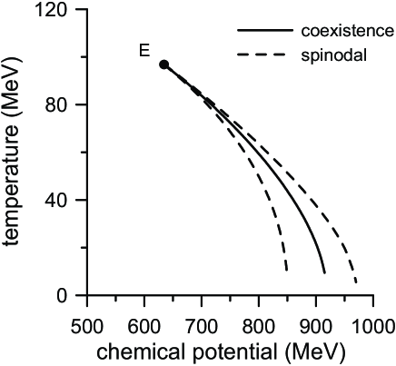
Figure 1: Phase diagram for the effective model in the $(\mu,T)$-plane, for $g=3.3$. The coexistence line ending at the critical point $E$ is represented by the full curve. The spinodal lines ($m_{\sigma}^{2}=0$) are shown as dashed curves.

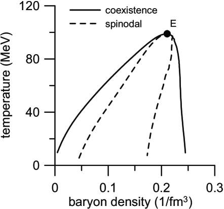
Figure 2: Phase diagram for the effective model in the $(n,T)$ plane, for $g=3.3$. Line conventions are the same as in Fig. 1. Inside the full curve the system is mechanically unstable.

The phase diagram in the $(n,T)$-plane is shown in Fig. 2. The phase border of the coexistence region is represented by the solid line and dashed lines stand for the spinodals. The sector between the lines on the right of the critical point $E$ corresponds to supercooled states in the chirally symmetric phase. Superheated states correspond to the area on the left. The domain inside the dashed lines corresponds to mechanically unstable states which undergo spinodal decomposition.

Results for the second choice of the coupling constant, $g=5.5$, are shown in Figs. 3 and 4. As we have mentioned, the difference of this case with respect to the first is that the coexistence line now reaches $\mu=0$. Because of this, the spinodals cross each other in the $(n,T)$ plane, and part of the phase coexistence region can be occupied by both supercooled and superheated states. Below the crossing no metastable states exist.

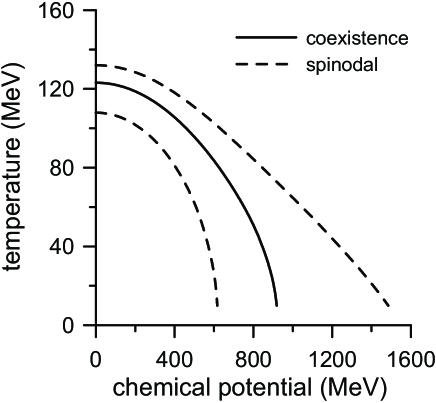
Figure 3: The same as Fig. 1 for $g=5.5$.

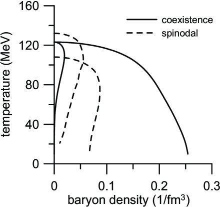
Figure 4: The same as Fig. 2 for $g=5.5$.

We have shown that the process of domain formation and growth in the phase conversion of strongly interacting matter from a chirally symmetric to a chirally broken state in an expanding QGP is dominated by the exponential increase of hydrodynamical sound-like modes, while chiral-like modes remain stable. We have mapped the boundaries of the unstable region for two illustrative cases, determining how much supercooling (or superheating) is necessary for the onset of spinodal instabilities.

In the case of relativistic heavy ion reactions, the short time scale of expansion and effects due to the finite size of the system could change significantly our results. In order to address these points one should perform extensive numerical simulations to study the development of instabilities in different scenarios. Results in this direction will be presented elsewhere.

- (1) F. Karsch, Nucl. Phys. A 698, 199 (2002).
- (2) J. Harris and B. Müller, Ann. Rev. Nucl. Part. Sci. 46, 71 (1996).
- (3) H.G. Ritter and X.N. Wang (ed), Proceedings of Quark Matter 2004, J. Phys. G 30 S633-S1425 (2004).
- (4) E.W. Kolb and M.S. Turner, The Early Universe (Addison-Wesley, Redwood City, 1990).
- (5) J.D. Gunton, M. San Miguel and P.S. Sahni in Phase Transitions and Critical Phenomena (Eds.: C. Domb and J. L. Lebowitz, Academic Press, London, 1983), v. 8.
- (6) J. Rafelski and J. Letessier, Phys. Rev. Lett. 85, 4695 (2000).
- (7) A. Dumitru and R.D. Pisarski, Nucl. Phys. A 698, 444 (2002).
- (8) O. Scavenius, A. Dumitru and A.D. Jackson, Phys. Rev. Lett. 87, 182302 (2001).
- (9) R.D. Pisarski, Phys. Rev. D 62, 111501 (2000); A. Dumitru and R. D. Pisarski, Phys. Lett. B 504, 282 (2001).
- (10) L.P. Csernai and I.N. Mishustin, Phys. Rev. Lett. 74, 5005 (1995); A. Abada and J. Aichelin, Phys. Rev. Lett. 74, 3130 (1995); A. Abada and M. C. Birse, Phys. Rev. D 55, 6887 (1997);
- (11) I.N. Mishustin and O. Scavenius, Phys. Rev. Lett. 83, 3134 (1999).
- (12) O. Scavenius and A. Dumitru, Phys. Rev. Lett. 83, 4697 (1999).
- (13) O. Scavenius, A. Dumitru, E.S. Fraga, J. T. Lenaghan and A. D. Jackson, Phys. Rev. D 63, 116003 (2001).
- (14) K. Paech, H. Stoecker and A. Dumitru, Phys. Rev. C 68, 044907 (2003); K. Paech and A. Dumitru, Phys. Lett. B 623, 200 (2005).
- (15) E.E. Zabrodin, L.V. Bravina, L.P. Csernai, H. Stocker and W. Greiner, Phys. Lett. B 423, 373 (1998).
- (16) P. Shukla and A. K. Mohanty, Phys. Rev. C 64, 054910 (2001).
- (17) C. Spieles, H. Stocker and C. Greiner, Phys. Rev. C 57, 908 (1998).
- (18) E.S. Fraga and R. Venugopalan, Physica A 345, 121 (2005); Braz. J. Phys. 34, 315 (2004).
- (19) J. Randrup, Phys. Rev. Lett. 92, 122301 (2004); J. Randrup, nucl-th/0406031; V. Koch, A. Majumder and J. Randrup, nucl-th/0509030.
- (20) E.S. Fraga and G. Krein, Phys. Lett. B 614, 181 (2005).
- (21) M.A. Stephanov, K. Rajagopal and E.V. Shuryak, Phys. Rev. Lett. 81, 4816 (1998); Phys. Rev. D 60, 114028 (1999).
- (22) M. A. Halasz, A. D. Jackson, R. E. Shrock, M. A. Stephanov and J. J. Verbaarschot, Phys. Rev. D 58, 096007 (1998); J. Berges and K. Rajagopal, Nucl. Phys. B 538, 215 (1999); T.M. Schwarz, S.P. Klevansky and G. Papp, Phys. Rev. C 60, 055205 (1999).
- (23) O. Scavenius, A. Mocsy, I. N. Mishustin and D.H. Rischke, Phys. Rev. C 64, 045202 (2001).
- (24) Z. Fodor and S.D. Katz, Phys. Lett. B 534, 87 (2002); JHEP 0203, 014 (2002).
- (25) C.R. Allton et al., Phys. Rev. D 66, 074507 (2002).
- (26) M. Gell-Mann and M. Levy, Nuovo Cim. 16, 705 (1960); R. D. Pisarski, Phys. Rev. Lett. 76, 3084 (1996).
- (27) R.D. Pisarski and F. Wilczek, Phys. Rev. D 29, 338 (1984).
- (28) J. Kapusta, Finite Temperature Field Theory (Cambridge University Press, Cambridge, 1989).
- (29) M. Bailyn, Phys. Rev. D 22, 267 (1980).
- (30) H.T. Elze, Y. Hama, T. Kodama, M. Makler and J. Rafelski, J. Phys. G 25, 1935 (1999).
- (31) H. A. R. Gonçalves, S. B. Duarte, T. Kodama and V. D’Avila, Astron. Space Science 194, 313 (1992); T. Kodama, R. Donangelo and M. Guidry, Int. J. Theor. Phys. C 9, 745 (1998).
- (32) H.T. Elze, T. Kodama, J. Rafelski, Phys. Rev. E 57, 4170 (1998).
- (33) D.T. Son, Phys. Rev. Lett. 84, 3771 (2000).