Relativistic Mean Field Theory for Deformed Nuclei with Pairing Correlations

Abstract

We develop a relativistic mean field (RMF) description of deformed nuclei with pairing correlations in the BCS approximation. The treatment of the pairing correlations for nuclei whose Fermi surfaces are close to the threshold of unbound states needs special attention. With this in mind, we use a delta function interaction for the pairing interaction to pick up those states whose wave functions are concentrated in the nuclear region and employ the standard BCS approximation for the single-particle states obtained from the RMF theory with deformation. We apply the RMF + BCS method to the Zr isotopes and obtain a good description of the binding energies and the nuclear radii of nuclei from the proton drip line to the neutron drip line.

1 Introduction

It is our strong desire to obtain a model valid for all nuclei, including unstable ones, from the proton drip line to the neutron drip line. The relativistic mean field (RMF) theory has been used to describe such nuclei with one parameter set in all mass regions [1, 2, 3]. We have to include deformation and pairing correlations into the RMF model for a suitable description of finite nuclei. There is an extended study of all the even-even nuclei over the entire mass region by Hirata et al. including only deformation [4]. This calculation provides a good account of all the nuclei and indicates that almost all nuclei, except for those with most of the magic numbers, are deformed. Their calculation, however, does not include pairing correlations, because the conventional BCS treatment with the constant pairing interaction is not able to treat the case in which the Fermi surface is close to the unbound threshold [4].

The pairing correlations, on the other hand, have been treated nicely in the framework of the relativistic Hartree-Bogoliubov (RHB) method by Meng et al. [5, 6]. They were able to treat nuclei near the unbound threshold in the RHB framework. They solved the RHB equation in the coordinate space with box boundary conditions. This method has been applied to many proton magic nuclei and is capable of describing many interesting features, such as the giant halo where the neutron density distribution extends far from the nuclear region. This method is, however, limited to spherical nuclei. When extended to deformed system, this method requires such great compuatation time that we are not able to make calculations for all the nuclei in the periodic table in a systematic manner.

Recently, there was an interesting suggestion made by Yadav et al. that using the delta function interaction in the BCS formalism with proper box boundary conditions can provide a good description of the proton magic nuclei [7]. Indeed, the calculated results obtained from the RMF+BCS method and those obtained in the RHB framework are nearly equal for those proton magic nuclei with spherical shapes. The justification of this method was provided by Sandulescu et al. by solving the resonance states and taking into account the width effect exactly in the non-relativistic Skyrme Hartree-Fock framework[8]. The applicability and justification of such a delta function interaction is also discussed extensively in a work by Dobaczewski et al.[9] and references therein, where it is shown in the context of HFB calculations that the use of a delta force in finite space simulates the effect of finite range interaction in a phenomenological manner and can take into account the effects of unbound states properly. It is very interesting, therefore, to apply this prescription to deformed nuclei.

The self-consistent RMF theory was first extended to treat deformed nuclei by Price et al.[10] and Gambhir et al.[11]. In Gambhir’s work, the nucleon wave functions and the meson fields are expanded in terms of the harmonic oscillator wave functions. We employ this method for the mean field part and replace the BCS part with a constant pairing interaction by one with a delta function interaction. The fact that we use the nuclear wave functions (in particular, we compute the overlap between occupied and unoccupied states), allows us to pick up states in the continuum whose wave functions are concentrated in the nuclear region. This method, at least, is effective for spherical nuclei and may also be effective for the deformed case. We mention that the relativistic Hartree-Bogoliubov theory was worked out using the expansion method for deformed nuclei [12].

In this paper, we formulate the RMF theory with the BCS method for pairing correlations. In §2, we present the RMF formalism with deformation and pairing. In §3, we apply the method to Zr isotopes from the proton drip line to the neutron drip line. We compare the calculated results with those obtained with the assumption of spherical shapes in RCHB and those obtained without including the pairing correlations. In §4, we provide the summary of the present work.

2 RMF with deformation and pairing

We present here the formulation of the RMF theory with deformation and pairing correlations. We employ the model Lagrangian density with nonlinear terms for both $\sigma$ and $\omega$ mesons, as described in detail in Ref. [2], which is given by

$$\begin{array}[]{lll}{\cal L}&=&\bar{\psi}(i\gamma^{\mu}\partial_{\mu}-M)\psi+\,\frac{\displaystyle 1}{\displaystyle 2}\partial_{\mu}\sigma\partial^{\mu}\sigma-\frac{\displaystyle 1}{\displaystyle 2}m_{\sigma}^{2}\sigma^{2}-\frac{\displaystyle 1}{\displaystyle 3}g_{2}\sigma^{3}-\frac{\displaystyle 1}{\displaystyle 4}g_{3}\sigma^{4}-g_{\sigma}\bar{\psi}\sigma\psi\\ &&-\frac{\displaystyle 1}{\displaystyle 4}\Omega_{\mu\nu}\Omega^{\mu\nu}+\frac{\displaystyle 1}{\displaystyle 2}m_{\omega}^{2}\omega_{\mu}\omega^{\mu}+\frac{\displaystyle 1}{\displaystyle 4}g_{4}(\omega_{\mu}\omega^{\mu})^{2}-g_{\omega}\bar{\psi}\gamma^{\mu}\psi\omega_{\mu}\\ &&-\frac{\displaystyle 1}{\displaystyle 4}{R^{a}}_{\mu\nu}{R^{a}}^{\mu\nu}+\frac{\displaystyle 1}{\displaystyle 2}m_{\rho}^{2}\rho^{a}_{\mu}\rho^{a\mu}-g_{\rho}\bar{\psi}\gamma_{\mu}\tau^{a}\psi\rho^{\mu a}\\ &&-\frac{\displaystyle 1}{\displaystyle 4}F_{\mu\nu}F^{\mu\nu}-e\bar{\psi}\gamma_{\mu}\frac{\displaystyle 1-\tau_{3}}{\displaystyle 2}A^{\mu}\psi,\\ \end{array}$$ (1)

where the field tensors of the vector mesons and of the electromagnetic field take the following forms:

$$\left\{\begin{array}[]{rl}\Omega_{\mu\nu}=&\partial_{\mu}\omega_{\nu}-\partial_{\nu}\omega_{\mu},\\ R^{a}_{\mu\nu}=&\partial_{\mu}\rho^{a}_{\nu}-\partial_{\nu}\rho^{a}_{\mu}-2g_{\rho}\epsilon^{abc}\rho^{b}_{\mu}\rho^{c}_{\nu},\\ F_{\mu\nu}=&\partial_{\mu}A_{\nu}-\partial_{\nu}A_{\mu},\end{array}\right.$$ (2)

and other symbols have their usual meanings.

The classical variational principle leads to the Dirac equation,

$$\left[-i\alpha\nabla+V({\bf r})+\beta\left(M+S({\bf r})\right)\right]~{}\psi_{i}=~{}\epsilon_{i}\psi_{i},$$ (3)

for the nucleon spinors and the Klein-Gordon equation,

$$\left\{\begin{array}[]{lll}\{-\Delta+m_{\sigma}^{2}\}\sigma({\bf r})&=&-g_{\sigma}\rho_{s}({\bf r})-g_{2}\sigma^{2}({\bf r})-g_{3}\sigma^{3}({\bf r}),\\ \ \{-\Delta+m_{\omega}^{2}\}\omega^{\mu}({\bf r})&=&g_{\omega}j^{\mu}({\bf r})+g_{4}\omega^{2}_{\mu}({\bf r})\omega^{\mu}({\bf r}),\\ \ \{-\Delta+m_{\rho}^{2}\}\rho^{a\mu}({\bf r})&=&g_{\rho}j^{a\mu}({\bf r}),\\ \ -\Delta A^{\mu}({\bf r})&=&ej^{\mu}_{p}({\bf r}),\end{array}\right.$$ (4)

for the mesons. Here, $V({\bf r})$ represents the vector potential

$$V({\bf r})=g_{\omega}\gamma^{\mu}\omega_{\mu}({\bf r})+g_{\rho}\tau^{a}\gamma^{\mu}\rho^{a}_{\mu}({\bf r})+e\frac{\displaystyle 1-\tau_{3}}{\displaystyle 2}\gamma^{\mu}A_{\mu}({\bf r}),$$ (5)

and $S({\bf r})$ is the scalar potential

$$S({\bf r})=g_{\sigma}\sigma({\bf r}).$$ (6)

For the mean field, the nucleon spinors provide the corresponding source terms:

$$\left\{\begin{array}[]{lll}\rho_{s}({\bf r})&=&\sum\limits_{i=1}^{A}\bar{\psi}_{i}~{}\psi_{i},\\ j^{\mu}({\bf r})&=&\sum\limits_{i=1}^{A}\bar{\psi}_{i}\gamma^{\mu}\psi_{i},\\ j^{a\mu}({\bf r})&=&\sum\limits_{i=1}^{A}\bar{\psi}_{i}\gamma^{\mu}\tau^{a}\psi_{i},\\ j^{\mu}_{p}({\bf r})&=&\sum\limits_{i=1}^{A}\bar{\psi}_{i}\gamma^{\mu}\frac{\displaystyle 1-\tau_{3}}{\displaystyle 2}\psi_{i}.\end{array}\right.$$ (7)

Here, the summations are taken over the valence nucleons only. It should be noted that as usual, the present approach ignores the contribution of negative energy states (i.e. no-sea approximation), which implies that the vacuum is not polarized. The coupled equations (3) and (4) are non-linear quantum field equations, and their exact solutions are very complicated. For this reason, the mean field approximation is generally used; i.e., the meson field operators in Eq. (3) are replaced by their expectation values. In this treatment, the nucleons are considered to move independently in the classical meson fields. The coupled equations are solved self-consistently by iteration.

The symmetries of the system simplify the calculations considerably. In all the systems considered in this work, there exists time reversal symmetry, so there are no currents in the nucleus and therefore the spatial vector components of $\omega^{\mu}$, $\rho^{a\mu}$ and $A^{\mu}$ vanish. This leaves only the time-like components, $\omega^{0}$, $\rho^{a0}$ and $A^{0}$. Charge conservation guarantees that only the 3-component of the isovector $\rho^{00}$ survives.

2.1 Axially symmetric case

The RMF theory was extended to treat deformed nuclei with axially symmetric shapes by Gambhir et al. [11]. To make clear the notation used, here a brief review of the RMF method for axially deformed nuclei is given.

Many deformed nuclei can be described with axially symmetric shapes. In this case, rotational symmetry is lost, and therefore the total angular momentum, $j$, is no longer a good quantum number. However, the densities are still invariant with respect to rotation about the symmetry axis, which is assumed to be the $z$-axis in the following. It is then useful to work with cylindrical coordinates: $x=r_{\bot}\cos\varphi,y=r_{\bot}\sin\varphi$ and $z$. For such nuclei, the Dirac equation can be reduced to a coupled set of partial differential equations in the two variables $z$ and $r_{\bot}$. In particular, the spinor $\psi_{i}$ with the index $i$ is now characterized by the quantum numbers $\Omega_{i},\pi_{i}$ and $t_{i}$, where $\Omega_{i}=m_{l_{i}}+m_{s_{i}}$ is the eigenvalue of the symmetry operator $J_{z}$, $\pi_{i}$ is the parity and $t_{i}$ is the isospin. The spinor can be written in the form

$$\psi_{i}({\bf r},t)=\left(\begin{array}[]{c}f_{i}({\bf r})\\ ig_{i}({\bf r})\end{array}\right)=\frac{\displaystyle 1}{\displaystyle\sqrt{2\pi}}\left(\begin{array}[]{l}f^{+}_{i}(z,r_{\bot})e^{i(\Omega_{i}-1/2)\varphi}\\ f^{-}_{i}(z,r_{\bot})e^{i(\Omega_{i}+1/2)\varphi}\\ ig^{+}_{i}(z,r_{\bot})e^{i(\Omega_{i}-1/2)\varphi}\\ ig^{-}_{i}(z,r_{\bot})e^{i(\Omega_{i}+1/2)\varphi}\end{array}\right)\chi_{t_{i}}(t).$$ (8)

The four components $f^{\pm}_{i}(z,r_{\bot})$ and $g^{\pm}_{i}(z,r_{\bot})$ obey the coupled Dirac equations. For each solution with positive $\Omega_{i}$, $\psi_{i}$, we have the time-reversed solution with the same energy, $\psi_{\bar{i}}=T\psi_{i}$, with the time reversal operator $T=-i\sigma_{y}K$ ($K$ being the complex conjugation). For nuclei with time reversal symmetry, the contributions to the densities of the two time reversed states, $i$ and $\bar{i}$, are identical. Therefore, we find the densities

$$\rho_{s,v}=2\sum_{i>0}\left((|f^{+}_{i}|^{2}+|f^{-}_{i}|^{2})\mp(|g^{+}_{i}|^{2}+|g^{-}_{i}|^{2})\right)$$ (9)

and, in a similar way, $\rho_{3}$ and $\rho_{c}$. The sum here runs over only states with positive $\Omega_{i}$. These densities serve as sources for the fields $\phi=\sigma,\omega^{0},\rho^{00}$ and $A^{0}$, which are determined by the Klein-Gordon equation in cylindrical coordinates.

To solve the RMF equations, the basis expansion method is used. We closely follow the details, presentation and notation of Ref. [13]. For the axially symmetric case, the spinors $f_{i}^{\pm}$ and $g_{i}^{\pm}$ in Eq. (8) are expanded in terms of the eigenfunctions of a deformed axially symmetric oscillator potential,

$$V_{\textrm{osc}}(z,r_{\bot})=\frac{1}{2}M\omega_{z}^{2}z^{2}+\frac{1}{2}M\omega^{2}_{\bot}r^{2}_{\bot}.$$ (10)

Then, imposing volume conservation, the two oscillator frequencies $\omega_{\bot}$ and $\omega_{z}$ can be expressed in terms of a deformation parameter, $\beta_{0}$: $\omega_{z}=\omega_{0}\exp\left(-\sqrt{\frac{5}{4\pi}}\beta_{0}\right)$ and $\omega_{\bot}=\omega_{0}\exp\left(+\frac{1}{2}\sqrt{\frac{5}{4\pi}}\beta_{0}\right)$.

The basis is now determined by the two constants $\omega_{0}$ and $\beta_{0}$. The eigenfunctions of the deformed harmonic oscillator potential are characterized by the quantum numbers, $|\alpha\rangle=|n_{z},n_{r},m_{l},m_{s}\rangle$, where $m_{l}$ and $m_{s}$ are the components of the orbital angular momentum and of the spin along the symmetry axis. The eigenvalue of $J_{z}$, which is a conserved quantity in these calculations, is $\Omega=m_{l}+m_{s}$. The parity is given by $\pi=(-)^{n_{z}+m_{l}}$.

The eigenfunctions of the deformed harmonic oscillator can be written explicitly as

$$\Phi_{\alpha}(z,r_{\bot},\varphi,s,t)=\phi_{n_{z}}(z)\phi_{n_{r}}^{m_{l}}(r_{\bot})\frac{\displaystyle 1}{\displaystyle\sqrt{2\pi}}e^{im_{l}\varphi}\chi_{m_{s}}(s)\chi_{t_{\alpha}}(t),$$ (11)

with

$$\begin{array}[]{l}\phi_{n_{z}}(z)=\frac{\displaystyle N_{n_{z}}}{\displaystyle\sqrt{b_{z}}}H_{n_{z}}(\zeta)e^{-\zeta^{2}/2},\\ \phi_{n_{r}}^{m_{l}}(r_{\bot})=\sqrt{2}\frac{\displaystyle N_{n_{r}}^{m_{l}}}{\displaystyle b_{\bot}}\eta^{m_{l}/2}L_{n_{r}}^{m_{l}}(\eta)e^{-\eta/2},\end{array}$$ (12)

where $\zeta=z/b_{z}$ and $\eta=r^{2}_{\bot}/b^{2}_{\bot}$. The polynomials $H_{n}(\zeta)$ and $L_{n}^{m}(\eta)$ are the Hermite polynomials and the associated Laguerre polynomials, as defined in Ref. [14]. The quantities $N_{n_{z}}$ and $N_{n_{r}}^{m_{l}}$ are normalization constants.

The spinors $f_{i}^{\pm}$ and $g_{i}^{\pm}$ in Eq. (8) are explicitly given by the following relations:

$$\left\{\begin{array}[]{lll}f^{+}_{i}(z,r_{\bot})&=&\sum\limits_{\alpha}^{\alpha_{\textrm{max}}}f_{\alpha}^{(i)}\phi_{n_{z}}(z)\phi_{n_{r}}^{(\Omega-1/2)}(r_{\bot}),\\ f^{-}_{i}(z,r_{\bot})&=&\sum\limits_{\alpha}^{\alpha_{\textrm{max}}}f_{\alpha}^{(i)}\phi_{n_{z}}(z)\phi_{n_{r}}^{(\Omega+1/2)}(r_{\bot}),\\ g^{+}_{i}(z,r_{\bot})&=&\sum\limits_{\beta}^{\beta_{\textrm{max}}}g_{\beta}^{(i)}\phi_{n_{z}}(z)\phi_{n_{r}}^{(\Omega-1/2)}(r_{\bot}),\\ g^{-}_{i}(z,r_{\bot})&=&\sum\limits_{\beta}^{\beta_{\textrm{max}}}g_{\beta}^{(i)}\phi_{n_{z}}(z)\phi_{n_{r}}^{(\Omega+1/2)}(r_{\bot}).\end{array}\right.$$ (13)

The quantum numbers $\alpha_{\textrm{max}}$ and $\beta_{\textrm{max}}$ are chosen in such a way that the corresponding major quantum numbers $N=n_{z}+2n_{\rho}+m_{l}$ are not larger than $N_{F}+1$ for the expansion of the small components and not larger than $N_{F}$ for the expansion of the large components.

2.2 Pairing with delta function interaction

Based on the single-particle spectrum calculated with the RMF method described above, we carry out a state-dependent BCS calculation [15, 16]. The gap equation has a standard form for all the single particle states,

$$\Delta_{k}=-\frac{\displaystyle 1}{\displaystyle 2}\sum_{k^{\prime}>0}\frac{\displaystyle\bar{V}_{kk^{\prime}}\Delta_{k^{\prime}}}{\displaystyle\sqrt{(\varepsilon_{k^{\prime}}-\lambda)^{2}+\Delta_{k^{\prime}}^{2}}},$$ (14)

where $\varepsilon_{k^{\prime}}$ is the single-particle energy and $\lambda$ is the Fermi energy. The particle number condition is given by $2\sum\limits_{k>0}v_{k}^{2}=N$. In the present work, we use a delta force for the pairing interaction,

$$V=-V_{0}\delta({\bf r_{1}}-{\bf r_{2}}),$$ (15)

with the same strength $V_{0}$ for both protons and neutrons. The pairing matrix element for the $\delta$-function force is given by

$$\begin{array}[]{lll}\bar{V}_{ij}&=&\langle i\bar{i}|V|j\bar{j}\rangle-\langle i\bar{i}|V|\bar{j}j\rangle=-V_{0}\int d^{3}r\,\left[\psi^{\dagger}_{i}\psi^{\dagger}_{\bar{i}}\psi_{j}\psi_{\bar{j}}-\psi^{\dagger}_{i}\psi^{\dagger}_{\bar{i}}\psi_{\bar{j}}\psi_{j}\right]\\ \end{array},$$ (16)

with the pairing energy defined by $E_{\textrm{pair}}=-\sum\limits_{k>0}\Delta_{k}u_{k}v_{k}$. Equations (3) and (4), the gap equations (14), and the total particle number condition $N$ for a given nucleus are solved self-consistently by iteration.

3 Numerical calculation for Zr isotopes

We apply the formalism to the Zr isotopes from the proton drip line to the neutron drip line. For the RMF Lagrangian, we use the $A$-dependent parameter set TMA [2, 18, 17]. The parameter values are as follows. The masses of nucleon, $\sigma$, $\omega$ and $\rho$ mesons are, respectively, $M=938.900\mbox{ MeV}$, $m_{\sigma}=519.151\mbox{ MeV}$, $m_{\omega}=781.950\mbox{ MeV}$, $m_{\rho}=768.100\mbox{ MeV}$. The effective strengths of the couplings between various mesons and nucleons have the values $g_{\sigma}=10.055+3.050/A^{0.4}$, $g_{\omega}=12.842+3.191/A^{0.4}$ and $g_{\rho}=3.800+4.644/A^{0.4}$. The nonlinear coupling strengths of the $\sigma$ meson are given by $g_{2}=-0.328-27.879/A^{0.4}\mbox{ (}\mbox{fm}^{-1}\mbox{)}$, and $g_{3}=38.862-184.191/A^{0.4}$, whereas the self-coupling of the $\omega$ field has the strength $g_{4}=151.590-378.004/A^{0.4}$. For the pairing interaction, we take the strength of the delta function interaction as $V_{0}=343.7\mbox{ MeV fm}^{3}$, which was obtained by requiring that the experimental value of the proton pairing gap in ⁹⁰Zr (1.714 MeV) be reproduced with a given energy cutoff ($E_{\textrm{max}}-\lambda\leq 8.0$ MeV).

Because in many nuclei we have several solutions at different equilibrium deformations with similar energies, it is difficult to select the ground-state configuration uniquely. The procedure we employed is as follows. The basis deformation $\beta_{0}$ is set equal to $\beta_{2m}$, following the results of Hirata et al. [4], in which a constrained calculation [19] was carried out for the quadrupole moment, $Q_{20}$, to obtain the lowest minimum in the energy curve of each nucleus.

The present calculation was performed by expansion in 14 oscillator shells for both the fermion fields and the boson fields. The convergence of this calculation has been tested with 20 shells for both the fermion fields and the boson fields. Following Ref. [11], we fix $\hbar\omega_{0}=41A^{-1/3}$ for fermions. In what follows, we discuss the details of our calculations and the numerical results for the Zr isotopes.

Table 1: The ground state properties of even Zr isotopes calculated with the parameter set TMA. Listed are the total binding energy, $B_{tot}$, the binding energy per nucleon, $B_{per}$ , charge, neutron, proton, and matter root mean square radii, $R_{c}$, $R_{n}$, $R_{p}$ and $R_{m}$, and the quadrupole deformation parameter for the neutron, proton and matter distributions, $\beta_{2n}$, $\beta_{2p}$ and $\beta_{2m}$, with $A$ the mass number and $N$ the neutron number.

$A$	$N$	$B_{tot}$	$B_{per}$	$R_{c}$	$R_{n}$	$R_{p}$	$R_{m}$	$\beta_{2n}$	$\beta_{2p}$	$\beta_{2m}$
78	38	639.089	8.193	4.3331	4.1496	4.2586	4.2058	0.480	0.507	0.494
80	40	667.668	8.346	4.3431	4.2048	4.2688	4.2369	0.489	0.506	0.498
82	42	692.014	8.439	4.4085	4.3134	4.3353	4.3241	0.589	0.579	0.584
84	44	716.742	8.533	4.2734	4.2081	4.1979	4.2033	-0.205	-0.210	-0.207
86	46	739.502	8.599	4.2694	4.2381	4.1938	4.2175	-0.148	-0.166	-0.156
88	48	762.784	8.668	4.2628	4.2618	4.1871	4.2280	0.002	0.003	0.002
90	50	784.859	8.721	4.2697	4.2969	4.1941	4.2515	0.000	0.000	0.000
92	52	797.819	8.672	4.3056	4.3678	4.2307	4.3087	-0.121	-0.137	-0.128
94	54	811.838	8.637	4.3504	4.4372	4.2762	4.3695	0.216	0.226	0.220
96	56	825.419	8.598	4.3832	4.5023	4.3095	4.4230	0.267	0.269	0.268
98	58	837.427	8.545	4.5171	4.6629	4.4456	4.5755	0.525	0.517	0.522
100	60	849.997	8.500	4.4694	4.6457	4.3972	4.5480	0.412	0.393	0.405
102	62	860.800	8.439	4.4896	4.6945	4.4177	4.5880	0.407	0.391	0.401
104	64	870.744	8.373	4.5117	4.7424	4.4402	4.6285	0.406	0.395	0.402
106	66	879.994	8.302	4.5357	4.7903	4.4646	4.6701	0.409	0.403	0.407
108	68	888.649	8.228	4.5579	4.8366	4.4872	4.7102	0.408	0.407	0.408
110	70	895.861	8.144	4.5930	4.8991	4.5228	4.7657	0.442	0.435	0.440
112	72	902.253	8.056	4.6302	4.9699	4.5606	4.8277	0.501	0.466	0.488
114	74	910.199	7.984	4.5182	4.9054	4.4468	4.7496	-0.169	-0.173	-0.170
116	76	916.310	7.899	4.5284	4.9396	4.4571	4.7788	-0.142	-0.156	-0.147
118	78	922.451	7.817	4.5189	4.9614	4.4475	4.7934	0.001	0.000	0.000
120	80	928.345	7.736	4.5364	4.9908	4.4653	4.8220	-0.001	-0.001	-0.001
122	82	933.816	7.654	4.5542	5.0184	4.4834	4.8495	0.000	0.000	0.000
124	84	933.842	7.531	4.5653	5.0909	4.4947	4.9065	-0.014	-0.009	-0.013
126	86	934.295	7.415	4.5980	5.1619	4.5279	4.9694	0.162	0.115	0.147
128	88	935.359	7.307	4.6488	5.2217	4.5794	5.0298	0.237	0.204	0.227
130	90	936.150	7.201	4.6746	5.2808	4.6057	5.0826	0.261	0.228	0.251
132	92	937.086	7.099	4.6606	5.3443	4.5914	5.1278	-0.232	-0.184	-0.218
134	94	937.686	6.998	4.6787	5.3932	4.6098	5.1718	-0.239	-0.188	-0.224
136	96	937.995	6.897	4.6960	5.4382	4.6274	5.2128	-0.241	-0.190	-0.226
138	98	938.148	6.798	4.7133	5.4808	4.6449	5.2522	-0.243	-0.190	-0.227
140	100	937.988	6.700	4.7314	5.5211	4.6632	5.2902	-0.244	-0.192	-0.229

3.1 Binding energy per nucleon and two neutron separation energy

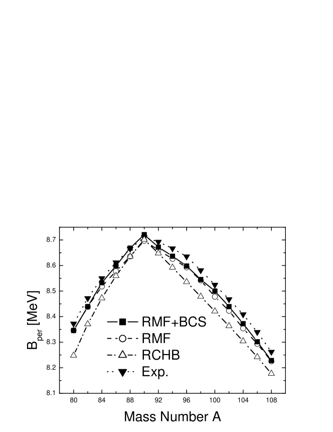
Figure 1: Binding energy per nucleon, $B_{per}$, for even Zr isotopes as functions of mass number $A$ obtained from the deformed RMF+BCS calculations (squares), the deformed RMF calculations (circles), the spherical RCHB calculations [20] (up triangles) and the experimental data [21] (down triangles).

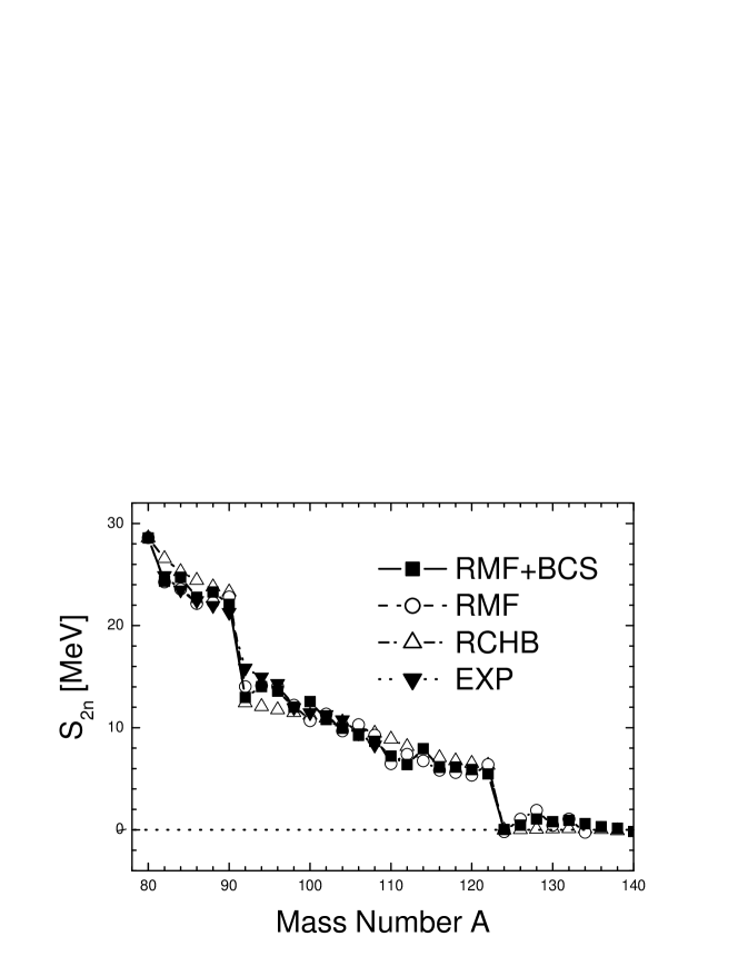
Figure 2: Two neutron separation energies, $S_{2n}$, for even Zr isotopes as functions of mass number $A$ obtained from the deformed RMF+BCS calculations (squares), the deformed RMF calculations (circles), the spherical RCHB calculations [20] (up triangles) and the experimental data [21] (down triangles).

The two neutron separation energy, $S_{2n}$, defined as

$$S_{2n}(Z,N)=B(Z,N)-B(Z,N-2),$$ (17)

is quite a sensitive quantity to test a microscopic theory, where $B(Z,N)$ is the binding energy of nuclei with proton number Z and neutron number N. The two neutron separation energy becomes negative when the nucleus becomes unstable with respect to two-neutron emission. Hence, the drip line nucleus for the corresponding isotope chain is the one with two less neutrons than the nucleus at which $S_{2n}$ first becomes negative.

In Figs. 1 and 2, we plot the results for the binding energy per nucleon of ^80-108Zr and the results for the two-neutron separation energies for the entire chain of Zr isotopes covering the proton and neutron drip lines. The figures also display the results of the RMF calculations, the results of the spherical RCHB calculations [20] and the available experimental data[21]. First, from Fig. 1, we can see that the RMF+BCS calculations give a better description of the binding energy per nucleon than the RMF calculations. The largest difference between the RMF+BCS results and the experimental values is less than $0.04$ MeV. Noting here that most of the nuclei are deformed and that despite this fact, we did not readjust any parameter for our calculations, the agreement is quite remarkable. Second, from Fig. 2, we see basically good agreement between experiment and the present calculation. The values of $S_{2n}$ for the so-called giant halos [20] (¹²⁴Zr$-$¹³⁸Zr) are reproduced accurately. The strong variation in the experimental separation energy at the neutron magic number $N=50$ is well accounted for by the present calculation. The small staggering for ⁸⁴Zr, ⁸⁸Zr, ¹⁰⁰Zr and ¹¹⁴Zr can be attributed to a mixture of the pairing interaction and the deformation effect. With the assumption of spherical shapes, it is predicted in Ref. [20] that the drip-line nucleus for Zr isotopes is ¹⁴⁰Zr. We also obtain ¹⁴⁰Zr as the drip-line nucleus. In both Figs. 1 and 2, the deformation effect is clearly seen. The deformed calculations describe the experimental data much better than the spherical calculations. This once again points out the need for an appropriate relativistic calculation with both deformation and proper pairing interaction taken into account in order to obtain a reliable description of all the nuclei from the proton drip line to the neutron drip line.

3.2 Root mean square neutron radii

The root mean square neutron radius is another basic important physical quantity to describe neutron-rich nuclei. In the mean field theory, the root mean square (rms) neutron radii can be directly deduced from the neutron density distributions, $\rho_{n}$:

$$R_{n}=\langle r^{2}_{n}\rangle^{1/2}=\left[\frac{\int\rho_{n}r^{2}d{\bf r}}{\int\rho_{n}d{\bf r}}\right]^{1/2}$$ (18)

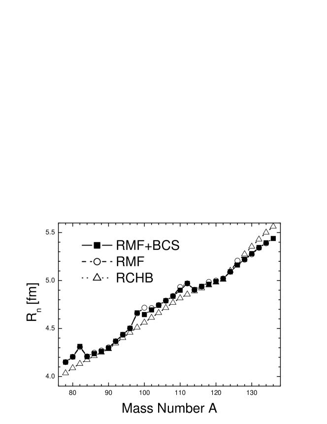
Figure 3: The root mean square neutron radii for even Zr isotopes as functions of mass number $A$ obtained from the deformed RMF+BCS calculations (squares), the deformed RMF calculations (circles), and the spherical RCHB calculations [20] (triangles).

In Fig. 3, the root mean square neutron radii for Zr nuclei are presented. Although the calculation was done with the assumption of spherical shapes, the results of RCHB [20] are also shown for comparison. Two interesting features are clearly seen. First, the so-called giant halos (¹²⁴Zr$-$¹³⁸Zr)[20] are obtained. Second, nuclei with large absolute values $\beta_{2m}$, ⁷⁸Zr$-$⁸²Zr and ⁹⁴Zr$-$¹¹²Zr (see also Table. 1 and Fig. 6), tend to have larger rms neutron radii. This can also be seen from the fact that some RMF results (for ¹⁰⁰Zr and ¹²⁶Zr) are larger than the RMF+BCS results.

Another point to note here is that despite the second effect mentioned above, for the so-called giant halos, the present work gives relatively small values for the root mean square neutron radii. We believe that this is due to the harmonic oscillator basis we used in the calculations of the deformed nuclei. This deficiency will be resolved in the near future, although a great deal of effort is necessary to change the numerical method. Nevertheless, despite the small discrepancies for giant halos, the present work provides good agreement with the RCHB[20] results and can give a reliable prediction of the rms neutron radii for all the nuclei from the proton drip line to the neutron drip line.

3.3 Single-particle states and their occupation probabilities

One interesting feature of exotic nuclei is the contribution from the continuum due to the pairing correlations. In this context, it is very interesting to study the amount by which the contributions from the continuum differ for the calculations with a constant pairing interaction and the calculations with a delta function interaction.

Figure 4: The occupation probability is represented by solid horizontal bar for each neutron single particle state of ¹²⁴Zr. The left panel displays the results of the RMF+BCS calculation with the delta function interaction, while the right panel displays the results of the constant pairing calculation. The dotted horizontal line represents the Fermi energy. In both panels, the occupation probabilities of the continuum states are multiplied by a factor of 5 for clarity.

Figure 5: The wave function $f(z,r_{\bot})$ for four typical resonant states in ¹²⁴Zr as functions of $r_{\bot}$ at $z=0.422$. The corresponding energy (in MeV) and occupation probability are, respectively, for $13/2^{+}[606],E=5.276\mbox{ and }v^{2}=0.005$; for $9/2^{-}[505],E=1.857\mbox{ and }v^{2}=0.041$; for $7/2^{-}[503],E=0.464\mbox{ and }v^{2}=0.196$ and for $5/2^{-}[503],E=1.683\mbox{ and }v^{2}=0.028$. The Nilsson quantum numbers in square brackets are determined using the dominant component in the expansion of this wave function in terms of the anisotropic oscillator basis.

In Fig. 4, we plot the occupation probabilities of ¹²⁴Zr for the neutron levels near the Fermi surface, i.e. in the interval $-10\mbox{ MeV}\leq E_{\textrm{s.p.}}\leq 8$ MeV. We present the occupation probabilities of neutron single-particle states for two cases, the delta function interaction and the constant pairing interaction usually used in the BCS framework. In the constant pairing calculation, we used $G_{n}=12.0/A$ and $G_{p}=30.0/A$, where $A$ is the mass number of ¹²⁴Zr, and the pairing window $\varepsilon_{i}-\lambda\leq 2(41A^{-1/3})$ [11]. Here, we used different pairing strengths, $G_{p}$ and $G_{n}$, for protons and neutrons in order to obtain similar gap energies, $\Delta$, than those obtained with the delta function interaction. We note that we use different pairing strengths for protons and neutrons because the level density around the Fermi surface is small for protons and large for neutrons, due to the continuum. The results obtained from the calculations using the delta function interaction and the constant pairing interaction are plotted in the left and right panels, respectively. Because in our calculation ¹²⁴Zr is almost spherical, we denote the corresponding spherical quantum number in the left panel. We can see all the spherical shell model states with small spin-orbit splitting in the positive energy region. They are all resonance states supported by the centrifugal potential. A recently performed resonant RMF+BCS calculation [22] yielded a quite similar spectrum for ¹²⁴Zr. It is thus seen that the contributions from the continuum states are very important. We see clearly that the BCS calculation with the delta function interaction can include more of the continuum states that are more localized inside the nuclear region, which correspond to resonance states. In addition, the delta function interaction includes a smaller contribution of the continuum states that are less localized in the pairing calculations. To see this point more clearly, we plot the corresponding resonant wave function $f$ in Fig. 5. It is easily seen that these states do have similar behavior as bound states. On the other hand, in the constant pairing case, the occupation probabilities decrease monotonically as functions of the single-particle energy.

We next point out an interesting feature of the vacancy between $E\approx 2\mbox{MeV}$ and $E\approx 5\mbox{MeV}$ in the single-particle spectra in the continuum seen in both calculations. If we performed calculations for the single-particle states in the coordinate space using box boundary conditions instead of the harmonic oscillator expansion method, we would obtain many states in the continuum. These are the so-called scattering states, which have small probabilities in the nuclear region. We do not obtain these scattering states, at least in the region of several MeV excitation energy in the continuum. Hence, we find that the single-particle states near the continuum threshold do have large probabilities in the nuclear region and contribute to the pairing correlations in nuclei close to the neutron drip line.

This unique feature of the delta function interaction in the BCS method is essential for the study of drip-line nuclei, where the Fermi energy is close to the threshold of the continuum. In this case, we have to estimate correctly the coupling between the bound states and the continuum states in order to pick up the resonance states, which have large amplitudes in the nuclear region. This would justify the use of such a simple RMF+BCS model to study all the nuclei, including the unstable ones from the proton drip line to the neutron drip line, as already demonstrated for the spherical case by Yadav et al. [7].

3.4 Effect of pairing on the deformation

The quadrupole moments of proton, neutron and nucleon distributions are calculated as

$$\begin{array}[]{lll}Q_{i}&=&\sqrt{\frac{\displaystyle 16\pi}{\displaystyle 5}}\langle r^{2}Y_{20}(\theta)\rangle_{i}\\ &=&\langle 2z^{2}-x^{2}-y^{2}\rangle_{i},\\ \end{array}$$ (19)

where $Y_{lm}$ represents the spherical harmonics, with $l$ being the multi-polarity. The index $i=p,n,m$ denotes the expectation value with respect to the proton, neutron and nucleon distributions, respectively.

The deformation parameters are defined in terms of the liquid drop model with uniform density. We expand the sharp surface of the liquid drop as

$$R_{i}(\theta)=R_{0}\left[1+\beta_{2i}Y_{20}(\theta)+\beta_{4i}Y_{40}(\theta)\right],$$ (20)

where $R_{0}=1.2A^{1/3}$ fm, in terms of the spherical harmonics under the assumption of axial symmetry. The quadrupole moment of the nucleon distribution in the liquid model is calculated as

$$Q_{m}^{\textrm{liq}}=\sqrt{\frac{\displaystyle 16\pi}{\displaystyle 5}}\frac{\displaystyle 3A}{\displaystyle 4\pi}R^{2}_{0}\beta_{2m},$$ (21)

dropping terms of higher order in $\beta_{\lambda m}$. The deformation parameter $\beta_{2m}$ is determined such that $Q_{m}^{\textrm{liq}}$ reproduces $Q_{m}$ in the RMF calculation, and is given by

$$\begin{array}[]{lll}\beta_{2m}&=&\frac{\displaystyle\sqrt{5\pi}}{\displaystyle 3}\frac{\displaystyle 1}{\displaystyle AR^{2}_{0}}Q_{m}\\ &=&\frac{\displaystyle\sqrt{5\pi}}{\displaystyle 3}\frac{\displaystyle 1}{\displaystyle AR^{2}_{0}}\langle 2z^{2}-x^{2}-y^{2}\rangle_{m}.\end{array}$$ (22)

The deformation parameters $\beta_{2p}$ and $\beta_{2n}$ are similarly given by

$$\beta_{2p}=\frac{\displaystyle\sqrt{5\pi}}{3}\frac{\displaystyle 1}{\displaystyle ZR^{2}_{0}}Q_{p},$$ (23)

$$\beta_{2n}=\frac{\displaystyle\sqrt{5\pi}}{3}\frac{\displaystyle 1}{\displaystyle NR^{2}_{0}}Q_{n}.$$ (24)

In the procedure to extract $\beta_{\lambda i}$ described above, we retain the linear relations between the moments and the deformation parameters so that it is easy to reproduce the moments from the deformation parameters in Table. 1. Regarding the determination of the deformation parameters with terms of higher order in $\beta_{\lambda i}$, we refer the reader to the description in Ref.[23].

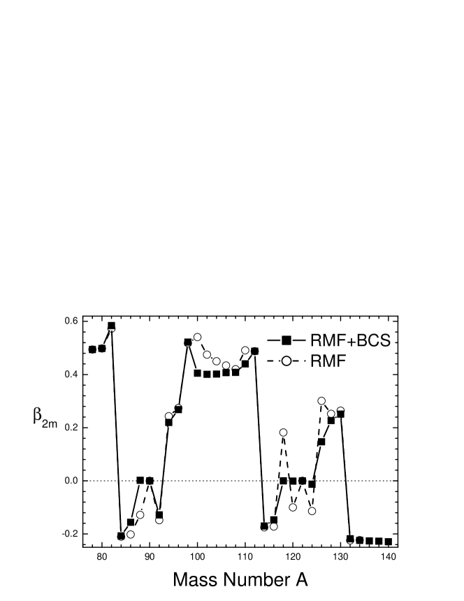
Figure 6: The quadrupole deformation, $\beta_{2m}$, for even Zr isotopes obtained from the deformed RMF+BCS (squares) and the deformed RMF (circles) calculations as functions of mass number $A$.

We plot in Fig. 6 the quadrupole deformation, $\beta_{2m}$, obtained from both the deformed RMF calculation and the deformed RMF+BCS calculation. It is easily seen that the pairing effect reduces the deformation of nuclei. More specifically, for some nuclei with $|\beta_{2m}|<0.2$ as found from the RMF calculation, (i.e. ⁸⁸Zr and ¹¹⁸Zr$-$¹²⁴Zr), the deformations are removed almost completely by the pairing effect. For other largely deformed nuclei (with $\beta_{2m}>0.3$), $\beta_{2m}$ is reduced somewhat, but not as much as in the case of their weakly deformed counterparts. In Fig. 7, we compared our predictions for the quadrupole deformation parameter $\beta^{2}_{2p}$ with the empirical values [24]. Except for ⁸²Zr, in which case our result is larger than the empirical value, the results are quantitively in good agreement with the empirical values.

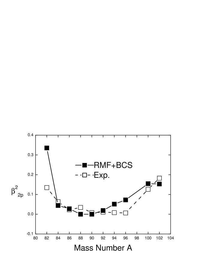
Figure 7: The square of the quadrupole deformation, $\beta^{2}_{2p}$, for even Zr isotopes obtained from the deformed RMF+BCS calculations (solid squares) and the empirical values [24] (empty squares) as functions of mass number $A$.

4 Conclusion

We have formulated the RMF theory with deformation and pairing. Conventionally, calculations for deformed nuclei are carried out using the expansion method in terms of the harmonic oscillator wave functions with pairing correlations treated using a constant pairing interaction with a pairing window. This method is, however, not applicable to the case of nuclei close to the neutron and proton drip lines, due to the importance of the resonance states in the continuum for such nuclei. In order to extend the RMF method so that it is applicable in these regions also, we introduced a delta function interaction for the pairing interaction, which allows the model to pick up resonant states by making the pairing matrix elements state dependent. The delta function description has been demonstrated to work for spherical nuclei.

In this paper, to demonstrate the applicability of the method, we have studied the Zr isotopes from the proton drip line to the neutron drip line. We calculated the binding energies, nuclear radii and deformation parameters of these nuclei. We also calculated the binding energy per nucleon and the two-neutron separation energy. We found that the agreement with experimental values is very satisfactory. The effect of deformation is clearly seen in these quantities as the large variation of the deformation as a function of mass number. We found that the neutron radii increase monotonically with the neutron number, with some anomalies, where the deformation changes suddenly. In our results, the so-called giant halo effect is preserved for nuclei close to the neutron drip line. The comparison of our results for $\beta^{2}_{2p}$ with the empirical values shows that our predictions for deformation parameters are quantitively in good agreement with the experimental results.

The occupation probabilities in the continuum are important for the purpose of determining if the present pairing method is effective in the treatment of the pairing in the continuum. While the occupation probabilities decrease monotonically as the states deviate from the Fermi energy in the case of a constant pairing interaction, they exhibit characteristic behavior for the case of a delta function interaction. The occupation probabilities are large for those states whose wave functions have large overlap with the wave functions below the Fermi surface. It would be interesting to compare our results with those of the Hartree-Bogoliubov calculations for these nuclei.

The deformation varies greatly for the Zr isotopes. The pairing correlations have the effect of reducing the deformation. This is clearly seen in our calculations. For those nuclei that have small deformations when calculated without pairing, the pairing correlations cause the nuclei to be spherical.

In conclusion, we have carried out calculations for the Zr isotopes to demonstrate that the presently considered RMF method with deformation and pairing correlations is effective even for nuclei close to the drip lines. It would be very interesting to make similar calculations for many nuclei in all mass regions with the present method.

5 Acknowledgements

We acknowledge fruitful discussions and collaborations with Prof. N. Sandulescu on the treatment of pairing in the continuum.

References

- [1] D. Hirata, H. Toki, T. Watabe, I. Tanihata and B. V. Carlson, Phys. Rev. C 44 (1991), 1467.
- [2] Y. Sugahara and H. Toki, Nucl. Phys. A 579 (1994), 557.
- [3] P. Ring, Prog. Part. Nucl. Phys. 37 (1996), 193.
- [4] D. Hirata, K. Sumiyoshi, I. Tanihata, Y. Sugahara, T. Tachibana and H. Toki, Nucl. Phys. A 616 (1997), 438c. D. Hirata, K. Sumiyoshi, I. Tanihata, Y. Sugahara and H. Toki, RIKEN-AF-NP-268 (1997).
- [5] J. Meng and P. Ring, Phys. Rev. Lett. 77 (1996), 3963.
- [6] J. Meng, Nucl. Phys. A 635 (1998), 3.
- [7] H. L. Yadav, S. Sugimoto and H. Toki, Mod. Phys. Lett. A 17 (2002), 2523.
- [8] N. Sandulescu, Nguyen Van Giai and R. J. Liotta, Phys. Rev. C 61 (2000), 061301(R).
- [9] J. Dobaczewski, W. Nazarewicz, T. R. Werner, J. F. Berger, C. R. Chinn and J. Dechargé, Phys. Rev. C 53 (1996), 2809.
- [10] C. E. Price and G. E. Walker, Phys. Rev. C 36 (1987), 354.
- [11] Y. K. Gambhir, P. Ring and A. Thimet, Ann. Phys. (N.Y.) 194 (1990), 132.
- [12] G. A. Lalazissis, D. Vretenar and P. Ring, Nucl. Phys. A 650 1999, 133.
- [13] P. Ring, Y. K. Gambhir and G. A. Lalazissis, Comput. Phys. Commun. 105 (1997), 77.
- [14] M. Abramowitz and I. A. Stegun, Handbook of Mathematical Functions (Dover, New York, 1970).
- [15] A. M. Lane, Nuclear Theory (Benjamin, 1964).
- [16] P. Ring and P. Schuck, The Nuclear Many-Body Problem (Springer, 1980).
- [17] Y. Sugahara, Doctor thesis in Tokyo Metropolitan University (1995).
- [18] H. Toki, D. Hirata, Y. Sugahara, K. Sumiyoshi and I. Tanihata, Nucl. Phys. A 588 (1995), 357c.
- [19] F. Floard et al., Nucl. Phys. A 203 (1973), 433.
- [20] J. Meng and P. Ring, Phys. Rev. Lett. 80 (1998), 460.
- [21] G. Audi and A. H. Wapstra, Nucl. Phys. A 595 (1995), 409.
- [22] N. Sandulescu, L. S. Geng, H. Toki, and G. Hillhouse, nucl-th/0306035.
- [23] N. Tajima, S. Takahara and N. Onishi, Nucl. Phys. A 603 (1996), 23.
- [24] S. Raman, C. W. Nestor, JR. and P. Tikkanen, At. Data Nucl. Data Tables 78 (2001), 1.