Electro and gamma nuclear physics in Geant4

Abstract

Adequate description of electro and gamma nuclear physics is of utmost importance in studies of electron beam-dumps and intense electron beam accelerators. I also is mandatory to describe neutron backgrounds and activation in linear colliders. This physics was elaborated in Geant4 over the last year, and now entered into the stage of practical application.

In the Geant4 Photo-nuclear data base there are at present about 50 nuclei for which the Photo-nuclear absorption cross sections have been measured. Of these, data on 14 nuclei are used to parametrize the gamma nuclear reaction cross-section The resulting cross section is a complex, factorized function of $A$ and $e=log(E_{\gamma})$, where $E_{\gamma}$ is the energy of the incident photon.

Electro-nuclear reactions are so closely connected with Photo-nuclear reactions that sometimes they are often called “Photo-nuclear”. The one-photon exchange mechanism dominates in Electro-nuclear reactions, and the electron can be substituted by a flux of photons. Folding this flux with the gamma-nuclear cross-section, we arrive at an acceptable description of the electro-nuclear physics.

Final states in gamma and electro nuclear physics are described using chiral invariant phase-space decay at low gamma or equivalent photon energies, and quark gluon string model at high energies.

We will present the modeling of this physics in Geant4, and show results from practical applications.

I Gamma nuclear reactions

I.1 Cross-section calculation

The Photo-nuclear cross sections parameterized in the Geant4 covers all incident photon energies from hadron production threshold up-wards. The parameterization is subdivided into five energy regions, each corresponding to the physical process that dominates. These are the Giant Dipole Resonance (GDR) region, the “quasi-deuteron” region, the $\Delta$ isobar region characterized by the dominant peak in the cross section which extends from the pion threshold to 450 MeV, the Roper resonance region that extends from roughly 450 MeV to 1.2 GeV, and the Reggeon-Pomeron region above 1.2 GeV.

From the Geant4geant4 Photo-nuclear data base currently 14 nuclei are used in defining the parameterization: ¹H, ²H, ⁴He, ⁶Li, ⁷Li, ⁹Be, ¹²C, ¹⁶O, ²⁷Al, ⁴⁰Ca, Cu, Sn, Pb, and U. The result is a function of $A$ and $e=log(E_{\gamma})$, where $E_{\gamma}$ is the incident photon energy. The cross-section is the sum of the components which parameterize each energy region.

The cross section in the GDR region can be described as the sum of two peaks,

$$GDR(e)=th(e,b_{1},s_{1})\cdot exp(c_{1}-p_{1}\cdot e)+$$

$$th(e,b_{2},s_{2})\cdot exp(c_{2}-p_{2}\cdot e).$$

The exponential describes the falling edge of the resonance which has power law behavior. The function

$$th(e,b_{i},s_{i})=\frac{1}{1+exp(\frac{b_{i}-e}{s_{i}})},$$ (1)

describes the rising edge of the resonance. It is the nuclear-barrier-reflection function and behaves like a threshold, cutting off the exponential. The exponential powers $p_{1}$ and $p_{2}$ are

$$p_{1}=1,p_{2}=2\mbox{\hskip 2.84526pt for \hskip 19.91692pt $A<4$ }$$

$$p_{1}=2,p_{2}=4\mbox{\hskip 2.84526pt for \hskip 2.84526pt $4\leq A<8$ }$$

$$p_{1}=3,p_{2}=6\mbox{\hskip 2.84526pt for $8\leq A<12$}$$

$$p_{1}=4,p_{2}=8\mbox{\hskip 2.84526pt for \hskip 17.07164pt $A\geq 12$}.$$

The $A$-dependent parameters $b_{i}$, $c_{i}$ and $s_{i}$ were found for each of the 14 nuclei and are interpolated for other nuclei.

The $\Delta$ isobar region was parameterized as

$$\Delta(e,d,f,g,r,q)=\frac{d\cdot th(e,f,g)}{1+r\cdot(e-q)^{2}},$$ (2)

where $d$ is an overall normalization factor. $q$ can be interpreted as the energy of the $\Delta$ isobar and $r$ as the inverse $\Delta$ width. $th$ is the threshold function. The $A$-dependence of these parameters is as follows:

• $d=0.41\cdot A$ (for ¹H it is 0.55, for ²H it is 0.88), i.e. the $\Delta$ yield is proportional to $A$;

• $f=5.13-.00075\cdot A$. $exp(f)$ shows how the pion threshold depends on $A$.

• $g=0.09$ for $A\geq 7$ and 0.04 for $A<7$;

• $q=5.84-\frac{.09}{1+.003\cdot A^{2}}$, which means that the “mass” of the $\Delta$ isobar moves to lower energies;

• $r=11.9-1.24\cdot log(A)$. $r$ is 18.0 for ¹H.

The $A$-dependence of the $f$, $q$ and $r$ parameters is due to the $\Delta+N\rightarrow N+N$ reaction, which can take place in the nuclear medium below the pion threshold.

The quasi-deuteron contribution was parameterized with the same form as the $\Delta$ contribution but without the threshold function:

$$QD(e,v,w,u)=\frac{v}{1+w\cdot(e-u)^{2}}.$$ (3)

For ¹H and ²H the quasi-deuteron contribution is almost zero. For these nuclei the third baryonic resonance was used instead, so the parameters for these two nuclei are quite different, but trivial. The parameter values are given below.

• $v=\frac{exp(-1.7+a\cdot 0.84)}{1+exp(7\cdot(2.38-a))}$, where $a=log(A)$. The $A$-dependence in the quasi-deuteron region is stronger than $A^{0.84}$ It contributes only little for light nuclei. For ¹H it is 0.078 and for ²H it is 0.08.

• $u=3.7$ and $w=0.4$. Experimental information is insufficient to fix their $A$-dependence. For both ¹H and ²H we have $u=6.93$ and $w=90$.

The Roper contribution was parameterized using the same form as the quasi-deuteron contribution:

$$Tr(e,v,w,u)=\frac{v}{1+w\cdot(e-u)^{2}}.$$ (4)

Using $a=log(A)$, the values of the parameters are

• $v=exp(-2.+a\cdot 0.84)$. For ¹H it is 0.22 and for ²H it is 0.34.

• $u=6.46+a\cdot 0.061$ (for ¹H and for ²H it is 6.57), so the Roper mass increases with $A$.

• $w=0.1+a\cdot 1.65$. For ¹H it is 20.0 and for ²H it is 15.0.

The Regge-Pomeron contribution was parametrized in terms of two exponentials describing the Pomeron and higher Reggeon contributions respectively:

$$RP(e,h)=h\cdot th(7.,0.2)\cdot(0.0116\cdot e^{(e\cdot 0.16)}+0.4\cdot e^{(-e\cdot 0.2)}),$$ (5)

with $h=A\cdot exp(-a\cdot(0.885+0.0048\cdot a))$.

I.2 Final state generation, low energies

For simulating final states for gamma-nuclear reactions, we are using the chiral invariant phase-space (CHIPS) approachCHIPS1 CHIPS2 CHIPS3 .

The CHIPS model uses a set of simple rules which govern microscopic quark-level behavior to model macroscopic hadronic systems. The invariant phase space distribution as a paradigm of thermalized chaos is applied to quarks, and simple kinematic mechanisms are used to model the hadronization of quarks into hadrons. Along with relativistic kinematics and the conservation of quantum numbers, the following concepts are introduced:

The Quasmon is any excited hadronic system, and can be viewed as a generalized hadron. At the constituent level, a Quasmon may be thought of as a bubble of quark-parton plasma in which the quarks are massless. The quark-partons in the Quasmon are massless and homogeneously distributed over the invariant phase space. It may also be considered as a bubble of the three-dimensional Feynman-Wilson Feynman-Wilson parton gas. The traditional hadron is a particle defined by quantum numbers and a fixed mass or width. The quark content of the hadron is a secondary concept constrained by the quantum numbers. The Quasmon, however, is defined by its quark content and mass, and the concept of a well defined particle with quantum numbers is of secondary importance.

The quark fusion hypothesis determines the rules of final state hadron production, with energy spectra reflecting the momentum distribution of the quarks in the system. Fusion occurs when a quark-partons in a Quasmon join to form a hadron. In cases of multiple Quasmon, quark-partons may be exchanged between the two Quasmons. Resulting hadrons are constrained to be produced on mass shell. The type of the outgoing hadron is selected using combinatoric and kinematic factors consistent with conservation laws.

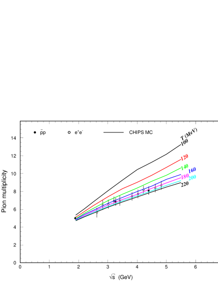
Figure 3: Average meson multiplicities in proton-antiproton and in electron-positron annihilation, as a function of the CMS energy of the interacting hadronic system. The points are experimental data Energy_Dep and the lines are CHIPS Monte Carlo calculations at several values of the critical temperature parameter $T$.

The only non-kinematic concept is the hypothesis of a critical temperature of the Quasmon. This has a 35-year history, starting with Ref. Hagedorn and is based on the experimental observation of regularities in the inclusive spectra of hadrons produced in different reactions at high energies. Qualitatively, the critical temperature hypothesis assumes that the Quasmon cannot be heated above a certain temperature. Adding more energy to the system increases only the number of constituent quark-partons while the temperature remains constant. The critical temperature $T_{c}=180-200$ MeV is the principal parameter of the model. The choice of this parameter is motivated from the results shown in Fig.3.

For the sake of briefness, we will only include the solution of the vacuum problem in this paper, and refer for the solution of the in-medium equations to the CHIPS publicationsCHIPS2 ,CHIPS3 .

I.2.1 Solution of the vacuum equations.

To generate hadron spectra from free Quasmons, the number of partons in the system must be found. For a finite system of $N$ partons with a total invariant mass $M$, the invariant phase space integral, $\Phi_{N}$, is proportional to $M^{2N-4}$. At a temperature $T$ the statistical density of states is proportional to $e^{-\frac{M}{T}}$ and the probability to find a system of $N$ quark-partons in a state with mass $M$ is $dW\propto M^{2N-4}e^{-\frac{M}{T}}dM$. For this kind of probability distribution the mean value of $M^{2}$ is

$$<M^{2}>=4N(N-1)\cdot T^{2}.$$ (6)

For large $N$ we obtain for massless particles the well-known $<M>\equiv\sqrt{<M^{2}>}=2NT$ result.

After a nucleon absorbs an incident quark-parton, such as a real or virtual photon, for example, the newly formed Quasmon has a total of $N$ quark-partons, where $N$ is determined by Eq. 6. Choosing one of these quark-partons with energy $k$ in the center of mass system (CMS) of $N$ partons, the spectrum of the remaining $N-1$ quark-partons is given by

$$\frac{dW}{kdk}\propto(M_{N-1})^{2N-6},$$ (7)

where $M_{N-1}$ is the effective mass of the $N-1$ quark-partons. The effective mass is a function of the total mass $M$,

$$M_{N-1}^{2}=M^{2}-2kM,$$ (8)

so that the resulting equation for the quark-parton spectrum is:

$$\frac{dW}{kdk}\propto(1-\frac{2k}{M})^{N-3}.$$ (9)

In order to decompose a Quasmon into a hadron and a residual Quasmon, one needs the probability of two quark-partons to produce the effective mass of the hadron. We calculate the spectrum of the second quark-parton by following the same argument used to determine Eq. 9. One quark-parton is chosen from the residual $N-1$. It has an energy $q$ in the CMS of the $N-1$ quark-partons. The spectrum is obtained by substituting $N-1$ for $N$ and $M_{N-1}$ for $M$ in Eq. 9 and then using Eq. 8 to get

$$\frac{dW}{qdq}\propto\left(1-\frac{2q}{M\sqrt{1-\frac{2k}{M}}}\right)^{N-4}.$$ (10)

To ensure that the fusion will result in a hadron of mass $\mu$, we apply the mass shell constraint for the outgoing hadron,

$$\mu^{2}=2\frac{k}{\sqrt{1-\frac{2k}{M}}}\cdot q\cdot(1-\cos\theta).$$ (11)

Here $\theta$ is the angle between the momenta k and q of the two quark-partons in the CMS of $N-1$ quarks. The kinematic quark fusion probability for any primary quark-parton with energy $k$ is then:

$$P(k,M,\mu)= \int\left(1-\frac{2q}{M\sqrt{1-\frac{2k}{M}}}\right)^{N-4}$$ (12)

$$\times\ \delta\left(\mu^{2}-\frac{2kq(1-\cos\theta)}{\sqrt{1-\frac{2k}{M}}}\right)qdqd\cos\theta.\ \ \ \$$

Using the $\delta$-function to perform the integration over $q$ one gets:

$$P(k,M,\mu)= \int\left(1-\frac{\mu^{2}}{Mk(1-\cos\theta)}\right)^{N-4}$$ (13)

$$\times\ \left(\frac{\mu^{2}\sqrt{1-\frac{2k}{M}}}{2k(1-\cos\theta)}\right)^{2}d\left(\frac{1-\cos\theta}{\mu^{2}}\right),\ \$$

or

$$P(k,M,\mu)= \frac{M-2k}{4k}\int\left(1-\frac{\mu^{2}}{Mk(1-\cos\theta)}\right)^{N-4}$$ (14)

$$\times\ d\left(1-\frac{\mu^{2}}{Mk(1-\cos\theta)}\right).$$

After the substitution $z=1-\frac{2q}{M_{N-1}}=1-\frac{\mu^{2}}{Mk(1-\cos\theta)}$, this becomes

$$P(k,M,\mu)=\frac{M-2k}{4k}\int z^{N-4}dz,$$ (15)

where the limits of integration are $0$ when $\cos\theta=1-\frac{\mu^{2}}{M\cdot k}$, and

$$z_{\max}=1-\frac{\mu^{2}}{2Mk},$$ (16)

when $\cos\theta=-1$. The resulting range of $\theta$ is therefore $-1<\cos\theta<1-\frac{\mu^{2}}{M\cdot k}$. Integrating from $0$ to $z$ yields

$$\frac{M-2k}{4k\cdot(N-3)}\cdot z^{N-3},$$ (17)

and integrating from $0$ to $z_{max}$ yields the total kinematic probability for hadronization of a quark-parton with energy $k$ into a hadron with mass $\mu$:

$$\frac{M-2k}{4k\cdot(N-3)}\cdot z_{\max}^{N-3}.$$ (18)

The ratio of expressions 17 and 18 can be treated as a random number, $R$, uniformly distributed on the interval [0,1]. Solving for $z$ then gives

$$z=\sqrt[N-3]{R}\cdot z_{\max}.$$ (19)

In addition to the kinematic selection of the two quark-partons in the fusion process, the quark content of the Quasmon and the spin of the candidate final hadron are used to determine the probability that a given type of hadron is produced. Because only the relative hadron formation probabilities are necessary, overall normalization factors can be dropped. Hence the relative probability can be written as

$$P_{h}(k,M,\mu)=(2s_{h}+1)\cdot z_{\max}^{N-3}\cdot C_{Q}^{h}.$$ (20)

Here, only the factor $z_{\max}^{N-3}$ is used since the other factors in equation 18 are constant for all candidates for the outgoing hadron. The factor $2s_{h}+1$ counts the spin states of a candidate hadron of spin $s_{h}$, and $C_{Q}^{h}$ is the number of ways the candidate hadron can be formed from combinations of the quarks within the Quasmon. In making these combinations, the standard quark wave functions for pions and kaons were used. For $\eta$ and $\eta^{\prime}$ mesons the quark wave functions $\eta=\frac{\bar{u}u+\bar{d}d}{2}-\frac{\bar{s}s}{\sqrt{2}}$ and $\eta^{\prime}=\frac{\bar{u}u+\bar{d}d}{2}+\frac{\bar{s}s}{\sqrt{2}}$ were used. No mixing was assumed for the $\omega$ and $\phi$ meson states, hence $\omega=\frac{\bar{u}u+\bar{d}d}{\sqrt{2}}$ and $\varphi=\bar{s}s$.

I.3 Final state generation, high energies

At high energies we use quark-gluon string model and a diffractive Ansatz for string excitation to describe the interactions of real and virtual photons with nuclei. A description of the means of doing this can be found in a separate paper in the present proceedingsStringstuff .

II Electro-nuclear scattering

Electro-nuclear reactions are very connected with Photo-nuclear reactions. They are sometimes called “Photo-nuclear” because the one-photon exchange mechanism dominates the reaction. In this sense electrons can be replaced by a flux of equivalent photons. This is not completely true, because at high energies diffractive mechanisms are possible, but these types of reactions are beyond the scope of this discussion.

II.1 Electro-nuclear cross-sections

The Equivalent Photon Approximation (EPA) was proposed by E. Fermi Fermi and developed by C. Weizsacker and E. Williams WeiWi and by L. Landau and E. Lifshitz LanLif . The covariant form of the EPA method was developed in Refs. Pomer and Grib . When using this method it is necessary to take into account that real photons are always transversely polarized while virtual photons may be longitudinally polarized. In general the differential cross section of the Electro-nuclear interaction can be written as

$$\frac{d^{2}\sigma}{dydQ^{2}}=\frac{\alpha}{\pi Q^{2}}(S_{TL}\cdot(\sigma_{T}+\sigma_{L})-S_{L}\cdot\sigma_{L}),$$ (21)

where

$$S_{TL}=y\frac{1-y+\frac{y^{2}}{2}+\frac{Q^{2}}{4E^{2}}-\frac{m^{2}_{e}}{Q^{2}}(y^{2}+\frac{Q^{2}}{E^{2}})}{y^{2}+\frac{Q^{2}}{E^{2}}},$$

$$S_{L}=\frac{y}{2}(1-\frac{2m_{e}^{2}}{Q^{2}}).$$

The differential cross section of the Electro-nuclear scattering can be rewritten as

$$\frac{d^{2}\sigma_{eA}}{dydQ^{2}}=\frac{\alpha y}{\pi Q^{2}}\left(\frac{(1-\frac{y}{2})^{2}}{y^{2}+\frac{Q^{2}}{E^{2}}}+\frac{1}{4}-\frac{m^{2}_{e}}{Q^{2}}\right)\sigma_{\gamma^{*}A},$$ (22)

where $\sigma_{\gamma^{*}A}=\sigma_{\gamma A}(\nu)$ for small $Q^{2}$ and is written as a function of $\epsilon$, $\nu$, and $Q^{2}$ for large $Q^{2}$. Interactions of longitudinal photons are normally included in the effective $\sigma_{\gamma^{*}A}$ cross section through the $\epsilon$ factor, but in the present method, the cross section of virtual photons is considered to be $\epsilon$-independent. The Electro-nuclear problem, with respect to the interaction of virtual photons with nuclei, can thus be split in two. At small $Q^{2}$ it is possible to use the $\sigma_{\gamma}(\nu)$ cross section. In the $Q^{2}>>m^{2}_{e}$ region it is necessary to calculate the effective $\sigma_{\gamma^{*}}(\epsilon,\nu,Q^{2})$ cross section.

Following the EPA notation, the differential cross section of Electro-nuclear scattering can be related to the number of equivalent photons $dn=\frac{d\sigma}{\sigma_{\gamma^{*}}}$. For $y<<1$ and $Q^{2}<4m^{2}_{e}$ the canonical method encs.eqPhotons leads to

$$\frac{ydn(y)}{dy}=-\frac{2\alpha}{\pi}ln(y).$$ (23)

In Budnev , integration over $Q^{2}$ for $\nu^{2}>>Q^{2}_{max}\simeq m^{2}_{e}$ leads to

$$\frac{ydn(y)}{dy}=-\frac{\alpha}{\pi}\left(\frac{1+(1-y)^{2}}{2}ln(\frac{y^{2}}{1-y})+(1-y)\right).$$ (24)

In the $y<<1$ limit this formula converges to Eq.(23). But the correspondence with Eq.(23) can be made more explicit if the exact integral

$$\frac{ydn(y)}{dy}=\frac{\alpha}{\pi}\left(\frac{1+(1-y)^{2}}{2}l_{1}-(1-y)l_{2}-\frac{(2-y)^{2}}{4}l_{3}\right),$$ (25)

where $l_{1}=ln\left(\frac{Q^{2}_{max}}{Q^{2}_{min}}\right)$, $l_{2}=1-\frac{Q^{2}_{max}}{Q^{2}_{min}}$, $l_{3}=ln\left(\frac{y^{2}+Q^{2}_{max}/E^{2}}{y^{2}+Q^{2}_{min}/E^{2}}\right)$, $Q^{2}_{min}=\frac{m_{e}^{2}y^{2}}{1-y}$, is calculated for $Q^{2}_{max(m_{e})}=\frac{4m^{2}_{e}}{1-y}$.

The factor $(1-y)$ is used arbitrarily to keep $Q^{2}_{max(m_{e})}>Q^{2}_{min}$, which can be considered as a boundary between the low and high $Q^{2}$ regions. The transverse photon flux can be calculated as an integral of Eq.(25) with the maximum possible upper limit

$$Q^{2}_{max(max)}=4E^{2}(1-y).$$ (26)

It can be approximated by

$$\frac{ydn(y)}{dy}=-\frac{2\alpha}{\pi}\left(\frac{(2-y)^{2}+y^{2}}{2}ln(\gamma)-1\right),$$ (27)

where $\gamma=\frac{E}{m_{e}}$. It must be pointed out that neither this approximation nor Eq.(25) works at $y\simeq 1$. The formal limit of the method is $y<1-\frac{1}{2\gamma}$.

Figure 1: Relative contribution of small $Q^{2}$ to the “photon flux” for (a) $1~{}GeV$ electrons and (b) $10~{}GeV$ electrons. In figures (c) and (d) the photon distribution $dn(\nu,Q^{2})$ is multiplied by the Photo-nuclear cross section and integrated over $Q^{2}$. The dashed lines are integrals over low $Q^{2}$ (under the dashed line in the first two figures), the solid lines are integrals over high-$Q^{2}$ (above the dashed lines in the first two figures).

Fig. 1(a,b) shows the energy distribution for the equivalent photons. The low-$Q^{2}$ flux is calculated using Eq.(23) (dashed lines) and Eq.(25) (dotted lines). The total flux is calculated using Eq.(27) (the solid lines) and using Eq.(25) with the upper limit defined by Eq.(26) (dash-dotted lines visible only around $\nu\approx E_{e}$). We find that to calculate the number of low-$Q^{2}$ equivalent photons or the total number of equivalent photons one can use the approximations given by Eq.(23) and Eq.(27), respectively, instead of using Eq.(25). Comparing the low-$Q^{2}$ photon flux and the total photon flux we find that the low-$Q^{2}$ photon flux is about half of the the total. From the interaction point of view the decrease of $\sigma_{\gamma*}$ with increasing $Q^{2}$ must be considered. The cross section reduction for the virtual photons with large $Q^{2}$ is governed by two factors. The cross section drops with $Q^{2}$ as the squared dipole nucleon form-factor

$$G^{2}_{D}(Q^{2})\approx\left(1+\frac{Q^{2}}{(843~{}MeV)^{2}}\right)^{-2},$$ (28)

and the thresholds the $\gamma A$ reactions are shifted to higher $\nu$ by a factor $\frac{Q^{2}}{2M}$, which is the difference between the $K$ and $\nu$ values. Following the method proposed in Brasse , $\sigma_{\gamma^{*}}$ at large $Q^{2}$ can be approximated as

$$\sigma_{\gamma*}=(1-x)\sigma_{\gamma}(K)G^{2}_{D}(Q^{2})e^{b(\epsilon,K)\cdot r+c(\epsilon,K)\cdot r^{3}},$$ (29)

where $r=\frac{1}{2}ln(\frac{Q^{2}+\nu^{2}}{K^{2}})$. The $\epsilon$-dependence of the $a(\epsilon,K)$ and $b(\epsilon,K)$ functions is weak, so for simplicity the $b(K)$ and $c(K)$ functions are averaged over $\epsilon$. They can be approximated as

$$b(K)\approx\left(\frac{K}{185~{}MeV}\right)^{0.85},c(K)\approx-\left(\frac{K}{1390~{}MeV}\right)^{3}.$$ (30)

The integrated photon flux folded with the cross section approximated by Eq.(29) is shown in Fig. 1(c,d). We show separately the low-$Q^{2}$ region ($Q^{2}<Q^{2}_{max(m_{e})}$, dashed lines), and the high-$Q^{2}$ region ($Q^{2}>Q^{2}_{max(m_{e})}$, solid lines). These functions will be integrated over $ln(\nu)$, hence because of the Giant Dipole Resonance contribution, the low-$Q^{2}$ part covers more than half the total $eA\rightarrow hadrons$ cross section. But at $\nu>200~{}MeV$, where the hadron multiplicity increases, the large $Q^{2}$ part dominates. In this sense, for a better simulation of the production of hadrons by electrons, it is necessary to simulate the high-$Q^{2}$ part as well as the low-$Q^{2}$ part.

Taking into account the contribution of high-$Q^{2}$ photons it is possible to use Eq.(27) with the over-estimated $\sigma_{\gamma^{*}A}=\sigma_{\gamma A}(\nu)$ cross section. The slightly over-estimated Electro-nuclear cross section is

$$\sigma^{*}_{eA}=(2ln(\gamma)-1)\cdot J_{1}-\frac{ln(\gamma)}{E_{e}}\left(2J_{2}-\frac{J_{3}}{E_{e}}\right).$$ (31)

where

$$J_{1}(E_{e})=\frac{\alpha}{\pi}\int^{E_{e}}\sigma_{\gamma A}(\nu)dln(\nu)$$ (32)

$$J_{2}(E_{e})=\frac{\alpha}{\pi}\int^{E_{e}}\nu\sigma_{\gamma A}(\nu)dln(\nu){\rm,\ and}$$ (33)

$$J_{3}(E_{e})=\frac{\alpha}{\pi}\int^{E_{e}}\nu^{2}\sigma_{\gamma A}(\nu)dln(\nu).$$ (34)

The equivalent photon energy $\nu=yE$ can be obtained for a particular random number $R$ from the equation

$$R=\frac{(2ln(\gamma)-1)J_{1}(\nu)-\frac{ln(\gamma)}{E_{e}}(2J_{2}(\nu)-\frac{J_{3}(\nu)}{E_{e}})}{(2ln(\gamma)-1)J_{1}(E_{e})-\frac{ln(\gamma)}{E_{e}}(2J_{2}(E_{e})-\frac{J_{3}(E_{e})}{E_{e}})}.$$ (35)

Eq.(25) is too complicated for the randomization of $Q^{2}$ but there is an easily randomized formula which approximates Eq.(25) above the hadronic threshold ($E>10~{}MeV$). It reads

$$\frac{\pi}{\alpha D(y)}\int^{Q^{2}}_{Q^{2}_{min}}\frac{ydn(y,Q^{2})}{dydQ^{2}}dQ^{2}=-L(y,Q^{2})-U(y),$$ (36)

where

$$L(y,Q^{2})=ln\left(F(y)+(e^{P(y)}-1+\frac{Q^{2}}{Q^{2}_{min}})^{-1}\right),$$ (37)

$$D(y)=1-y+\frac{y^{2}}{2}{\rm,\ and}$$ (38)

$$U(y)=P(y)\cdot\left(1-\frac{Q^{2}_{min}}{Q^{2}_{max}}\right){\rm,\ with}$$ (39)

$$F(y)=\frac{(2-y)(2-2y)}{y^{2}}\cdot\frac{Q^{2}_{min}}{Q^{2}_{max}}{\rm,\ and}$$ (40)

$$P(y)=\frac{1-y}{D(y)}.$$ (41)

The $Q^{2}$ value can then be calculated as

$$\frac{Q^{2}}{Q^{2}_{min}}=1-e^{P(y)}+\left(e^{R\cdot L(y,Q^{2}_{max})-(1-R)\cdot U(y)}-F(y)\right)^{-1},$$ (42)

where $R$ is a random number. In Fig. 2, Eq.(25) (solid curve) is compared to Eq.(36) (dashed curve). Because the two curves are almost indistinguishable in the figure, this can be used as an illustration of the $Q^{2}$ spectrum of virtual photons, which is the derivative of these curves. An alternative approach is to use Eq.(25) for the randomization with a three dimensional table $\frac{ydn}{dy}(Q^{2},y,E_{e})$.

Figure 2: Integrals of $Q^{2}$ spectra of virtual photons for three energies $10~{}MeV$, $100~{}MeV$, and $1~{}GeV$ at $y=0.001$, $y=0.5$, and $y=0.95$. The solid line corresponds to Eq.(25) and the dashed line (which almost everywhere coincides with the solid line) corresponds to Eq.(25).

After the $\nu$ and $Q^{2}$ values have been found, the value of $\sigma_{\gamma^{*}A}(\nu,Q^{2})$ is calculated using Eq.(29). Note that if $R\cdot\sigma_{\gamma A}(\nu)>\sigma_{\gamma^{*}A}(\nu,Q^{2})$, no interaction occurs and the electron keeps going.

II.2 Final state generation

Final states are generated using the single photon exchange assumption. Sampling the equivalent photon distribution described in the previous section allows to construct an exchange particle that in turn can be treated by the mechanisms used for gamma nuclear scattering. The question to be answered is that of the absorption mechanisms of these particles in the context of parton exchange diagrams.

In the example of the Photo-nuclear reaction discussed in the comparison section, namely the description of $90^{\circ}$ proton and deuteron spectra in $A({\gamma},X)$ reactions at $E_{\gamma}=59-65$ MeV, the assumption on the initial Quasmon excitation mechanism was the same. The description of the $90^{\circ}$ data was satisfactory, but the generated data showed very little angular dependence, as the velocity of Quasmons produced in the initial state was small, and the fragmentation process was almost isotropic. Experimentally, the angular dependence of secondary protons in photo-nuclear reactions is quite strong even at low energies (see, for example, Ref. Ryckebusch ). This is a challenging experimental fact which is difficult to explain in any model. It’s enough to say that if the angular dependence of secondary protons in the $\gamma^{40}$Ca interaction at 60 MeV is analyzed in terms of relativistic boost, then the velocity of the source should reach $0.33c$; hence the mass of the source should be less than pion mass. The main subject of the present publication is to show that the quark-exchange mechanism used in the CHIPS model can not only model the clusterization of nucleons in nuclei and hadronization of intra-nuclear excitations into nuclear fragments, but can also model complicated mechanisms of interaction of photons and hadrons in nuclear matter.

Quark-exchange diagrams help to keep track of the kinematics of the quark-exchange process To apply the mechanism to the first interaction of a photon with a nucleus, it is necessary to assume that the quark-exchange process takes place in nuclei continuously, even without any external interaction. Nucleons with high momenta do not leave the nucleus because of the lack of excess energy. The hypothesis of the CHIPS model is that the quark-exchange forces between nucleons NN QEX  continuously create clusters in normal nuclei. Since a low-energy photon (below the pion production threshold) cannot be absorbed by a free nucleon, other absorption mechanisms involving more than one nucleon have to be used.

The simplest scenario is photon absorption by a quark-parton in the nucleon. At low energies and in vacuum this does not work because there is no corresponding excited baryonic state. But in nuclear matter there is a possibility to exchange this quark with a neighboring nucleon or a nuclear cluster. The diagram for the process is shown in the upper part of Fig. 4. In this case the photon is absorbed by a quark-parton from the parent cluster $\rm{PC}_{1}$, and then the secondary nucleon or cluster $\rm{PC}_{2}$ absorbs the entire momentum of the quark and photon. The exchange quark-parton $q$ restores the balance of color, producing the final-state hadron F and the residual Quasmon RQ. The process looks like a knockout of a quasi-free nucleon or cluster out of the nucleus. It should be emphasized that in this scenario the CHIPS event generator produces not only “quasi-free” nucleons but “quasi-free” fragments too. The yield of these quasi-free nucleons or fragments is concentrated in the forward direction.

The second scenario, shown in the lower part of Fig.4 which provides for an angular dependence is the absorption of the photon by a colored fragment ($\rm{CF}_{2}$ in Fig. 4). In this scenario, both the primary quark-parton with momentum $k$ and the photon with momentum $q_{\gamma}$ are absorbed by a parent cluster ($\rm{PC}_{2}$ in the lower part of Fig. 4), and the recoil quark-parton with momentum $q$ cannot fully compensate the momentum $k+q_{\gamma}$. As a result the radiation of the secondary fragment in the forward direction becomes more probable.

In both cases the angular dependence is defined by the first act of hadronization. The further fragmentation of the residual Quasmon is almost isotropic.

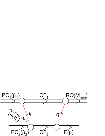
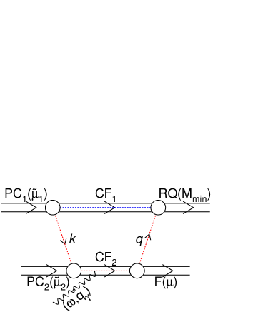
Figure 4: Diagrams of photon absorption in the quark exchange mechanism. $\rm{PC}_{1,2}$ are the parent clusters with bound masses $\tilde{\mu}_{1,2}$, involved in the quark-exchange. $\rm{CF}_{1,2}$ are the colored nuclear fragments. F($\mu$) is the outgoing hadron with mass $\mu$. RQ is the residual Quasmon which carries the rest of the excitation energy and momentum. $M_{\min}$ characterizes its minimum mass defined by its quark content. Dashed lines indicate colored objects. The photon is absorbed by a quark-parton $k$ from the parent cluster $\rm{PC}_{1}$.

It was shown in above that the energy spectrum of quark partons in a Quasmon can be calculated as

$$\frac{dW}{k^{\ast}dk^{\ast}}\propto\left(1-\frac{2k^{\ast}}{M}\right)^{N-3},$$ (43)

where $k^{\ast}$ is the energy of the primary quark-parton in the Center of Mass System (CMS) of the Quasmon, $M$ is the mass of the Quasmon, and $N$, the number of quark-partons in the Quasmon, can be calculated from the equation

$$<M^{2}>=4\cdot N\cdot(N-1)\cdot T^{2}.$$ (44)

Here $T$ is the temperature of the system.

In the first scenario of the $\gamma A$ interaction (Fig. 4), as both interacting particles are massless, we assumed that the cross section for the interaction of the photon with a particular quark-parton is proportional to the charge of the quark-parton squared, and inversely proportional to the mass of the photon-parton system $s$, which can be calculated as

$$s=2\omega k(1-\cos(\theta_{k})).$$ (45)

Here $\omega$ is the energy of the photon, and $k$ is the energy of the quark-parton in the Laboratory System (LS):

$$k=k^{\ast}\cdot\frac{E_{N}+p_{N}\cdot\cos(\theta_{k})}{M_{N}}.$$ (46)

In the case of a virtual photon, equation (45) can be written as

$$s=2k(\omega-q_{\gamma}\cdot\cos(\theta_{k})),$$ (47)

where $q_{\gamma}$ is the momentum of the virtual photon. In both cases equation (43) transforms into

$$\frac{dW}{dk^{\ast}}\propto\left(1-\frac{2k^{\ast}}{M}\right)^{N-3},$$ (48)

and the angular distribution in $\cos(\theta_{k})$ converges to a $\delta$-function: in the case of a real photon $\cos(\theta_{k})=1$, and in the case of a virtual photon $\cos(\theta_{k})=\frac{\omega}{q_{\gamma}}$.

In the second scenario for the photon interaction (lower part of Fig. 4) we assumed that both the photon and the primary quark-parton, randomized according to equation (43), enter the parent cluster $\rm{PC}_{2}$, and after that the normal procedure of quark exchange continues, in which the recoiling quark-parton $q$ returns to the first cluster.

An additional parameter in the model is the relative contribution of both mechanisms. As a first approximation we assumed equal probability, but in the future, when more detailed data are obtained, this parameter can be adjusted.

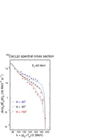
Figure 5: Comparison of the CHIPS model results (lines in the figure) with the experimental data Ryckbosch on proton spectra at $90^{\circ}$ in the Photo-nuclear reactions on ⁴⁰Ca at 59–65 MeV (open circles), and proton spectra at $60^{\circ}$ (triangles) and $150^{\circ}$ (diamonds). Statistical errors in the CHIPS results are not shown but can be judged by the point-to-point variations in the lines. The comparison is absolute, using the value of total Photo-nuclear cross section of 5.4 mb for Ca, as given in Ref. Ahrens .

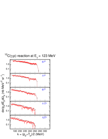
Figure 6: Comparison of the CHIPS model results (lines in the figure) with the experimental data Harty on proton spectra at $57^{\circ}$, $77^{\circ}$, $97^{\circ}$, $117^{\circ}$, and $127^{\circ}$ in the Photo-nuclear reactions on ¹²C at 123 MeV (open circles). The value of the total Photo-nuclear cross section was set at 1.8 mb.

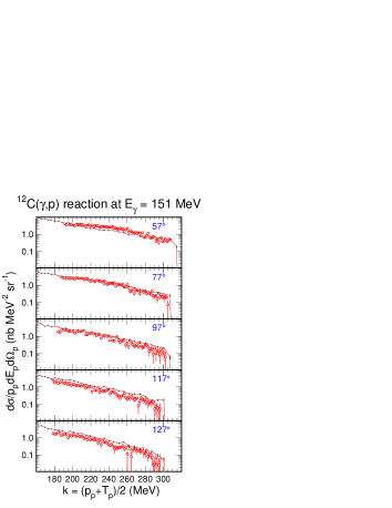
Figure 7: Same as in Fig. 6, for the photon energy 151 MeV.

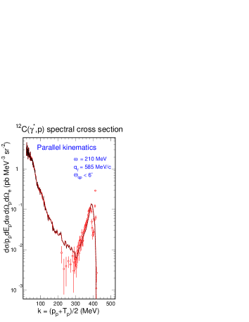
Figure 8: Comparison of the CHIPS model results (line in the figure) with the experimental data Bates (open circles) on the proton spectrum measured in parallel kinematics in the ¹²C(e,e^′p) reaction at an energy transfer equal to 210 MeV and momentum transfer equal to 585 MeV/$c$. Statistical errors in the CHIPS result are not shown but can be judged by the point-to-point variations in the line. The relative normalization is arbitrary.

III Comparison with experiment

We begin the comparison with the data on proton production in the ⁴⁰Ca$(\gamma,X)$ reaction at $90^{\circ}$ at 59–65 MeV Ryckbosch , and at $60^{\circ}$ and $150^{\circ}$ at 60 MeV Abeele . We analyzed these data together to compare the angular dependence generated by CHIPS with experimental data. The data are presented as a function of the invariant inclusive cross section $f=\frac{d\sigma}{p_{p}dE_{p}}$ depending on the variable $k=\frac{T_{p}+p_{p}}{2}$, where $T_{p}$ and $p_{p}$ are the kinetic energy and the momentum of the secondary proton. As one can see from Fig. 5, the angular dependence of the proton yield in photo-production on ⁴⁰Ca at $60$ MeV is reproduced quite well by the CHIPS event generator.

The second set of measurements that we use for the benchmark comparison deals with the secondary proton yields in ¹²C$(\gamma,X)$ reactions at 123 and 151 MeV Harty , which is still below the pion production threshold on a free nucleon. Inclusive spectra of protons have been measured in $\gamma^{12}$C reactions at $57^{\circ}$, $77^{\circ}$, $97^{\circ}$, $117^{\circ}$, and $127^{\circ}$. Originally, these data were presented as a function of the missing energy. We present the data in Figs. 6 and 7 together with CHIPS calculations in the form of the invariant inclusive cross section dependent on $k$.

The agreement between the experimental data and the CHIPS model results is quite remarkable. Both data and calculations show significant strength in the proton yield cross section up to the kinematic limits of the reaction. The angular distribution in the model is not as prominent as in the experimental data, but agrees well qualitatively.

Using the same parameters, we applied the CHIPS event generator to the ¹²C(e,e^′p) reaction measured in Ref.Bates . The proton spectra were measured in parallel kinematics in the interaction of virtual photons with energy $\omega=210$ MeV and momentum $q_{\gamma}=585$ MeV/$c$. To account for the experimental conditions in the CHIPS event generator, we have selected protons generated in the forward direction with respect to the direction of the virtual photon, with the relative angle $\Theta_{qp}<6^{\circ}$. The CHIPS generated distribution and the experimental data are shown in Fig. 8 in the form of the invariant inclusive cross section as a function of $k$. The CHIPS event generator works only with ground states of nuclei so we did not expect any narrow peaks for ${}^{1}p_{3/2}$-shell knockout or for other shells. Nevertheless we found that the CHIPS event generator fills in the so-called “${}^{1}s_{1/2}$-shell knockout” region, which is usually artificially smeared by a Lorentzian Lorentzian . In the regular fragmentation scenario the spectrum of protons below $k=300$ MeV is normal; it falls down to the kinematic limit. The additional yield at $k>300$ MeV is a reflection of the specific first act of hadronization with the quark exchange kinematics. The slope increase with momentum is approximated well by the model, but it is obvious that the yield close to the kinematic limit of the $2\rightarrow 2$ reaction can only be described in detail if the excited states of the residual nucleus are taken into account.

The angular dependence of the proton yield in low-energy photo-nuclear reactions is described in the CHIPS model and event generator. The most important assumption in the description is the hypothesis of a direct interaction of the photon with an asymptotically free quark in the nucleus, even at low energies. This means that asymptotic freedom of QCD and dispersion sum rules sum_rules can in some way be generalized for low energies. The knockout of a proton from a nuclear shell or the homogeneous distributions of nuclear evaporation cannot explain significant angular dependences at low energies.

The same mechanism appears to be capable of modeling proton yields in such reactions as the ¹⁶C(e,e^′p) reaction measured at MIT Bates Bates , where it was shown that the region of missing energy above 50 MeV reflects “two-or-more-particle knockout” (or the “continuum” in terms of the shell model). The CHIPS model may help to understand and model such phenomena.

- (1) E. Fermi, Z. Physik 29, 315 (1924).
- (2) K. F. von Weizsacker, Z. Physik 88, 612 (1934), E. J. Williams, Phys. Rev. 45, 729 (1934).
- (3) L. D. Landau and E. M. Lifshitz, Soc. Phys. 6, 244 (1934).
- (4) I. Ya. Pomeranchuk and I. M. Shmushkevich, Nucl. Phys. 23, 1295 (1961).
- (5) V. N. Gribov et al., ZhETF 41, 1834 (1961).
- (6) L. D. Landau, E. M. Lifshitz, “Course of Theoretical Physics” v.4, part 1, “Relativistic Quantum Theory”, Pergamon Press, p. 351, The method of equivalent photons.
- (7) V. M. Budnev et al., Phys. Rep. 15, 181 (1975).
- (8) F. W. Brasse et al., Nucl. Phys. B 110, 413 (1976).
- (9) P. V. Degtyarenko, M. V. Kossov, and H.P. Wellisch, Chiral invariant phase space event generator, I. Nucleon-antinucleon annihilation at rest, Eur. Phys. J. A 8, 217-222 (2000).
- (10) P. V. Degtyarenko, M. V. Kossov, and H. P. Wellisch, Chiral invariant phase space event generator, II.Nuclear pion capture at rest, Eur. Phys. J. A 9, (2001).
- (11) P. V. Degtyarenko, M. V. Kossov, and H. P. Wellisch, Chiral invariant phase space event generator, III Photo-nuclear reactions below (3,3) excitation, Eur. Phys. J. A 9, (2001).
- (12) K.G. Wilson, Proc. Fourteenth Scottish Universities Summer School in Physics (1973), eds R. L. Crawford, R. Jennings (Academic Press, New York, 1974)
- (13) R. Hagedorn, Nuovo Cimento Suppl. 3 (1965) 147
- (14) P. Gregory et al., Nucl. Phys. B 102 (1976) 189
- (15) K. Maltman and N. Isgur, Phys. Rev. D 29 (1984) 952.
- (16) L. D. Landau, E. M. Lifshitz, “Course of Theoretical Physics” v.4, part 1, “Relativistic Quantum Theory”, Pergamon Press, paragraph 96, The method of equivalent photons.
- (17) C. Bernard, A. Duncan, J. LoSecco, and S. Weinberg, Phys. Rev. D 12 (1975) 792; E. Poggio, H. Quinn, and S. Weinberg, Phys. Rev. D 13 (1976) 1958
- (18) D. Ryckbosch et al., Phys. Rev. C 42 (1990) 444.
- (19) J. Ahrens et al., Nucl. Phys. A446 (1985) 229c.
- (20) Jan Ryckebusch et al., Phys. Rev. C 49 (1994) 2704.
- (21) C. Van den Abeele; private communication cited in the reference: Jan Ryckebusch et al., Phys. Rev. C 49 (1994) 2704.
- (22) P.D. Harty et al. (unpublished); private communication cited in the reference: Jan Ryckebusch et al., Phys. Rev. C 49 (1994) 2704.
- (23) L.B. Weinstein et al., Phys. Rev. Lett. 64 (1990) 1646.
- (24) J.P. Jeukenne and C. Mahaux, Nucl. Phys. A 394 (1983) 445.
- (25) G. Folger, J.P. Wellisch, String parton models in Geant4, Proceedings of Computing in High Energy and Nuclear Physics, La Jolla, California, March 24-28, 2003.
- (26) Geant4: A simulation toolkit, By Geant4 (S.Agostinelli at al.) SLAC-PUB-9350, Aug 2002.