A Self-Consistent Solution to the Nuclear Many-Body Problem at Finite Temperature

Abstract

The properties of symmetric nuclear matter are investigated within the Green’s functions approach. We have implemented an iterative procedure allowing for a self-consistent evaluation of the single-particle and two-particle propagators. The in-medium scattering equation is solved for a realistic (non-separable) nucleon-nucleon interaction including both particle-particle and hole-hole propagation. The corresponding two-particle propagator is constructed explicitely from the single-particle spectral functions. Results are obtained for finite temperatures and an extrapolation to T=0 is presented.

I Introduction

The evaluation of the saturation properties of nuclear matter from realistic models of the nucleon-nucleon (NN) interaction is one of the challenging testing grounds for many-body theories of quantum systemsbaldo99 ; muether00 . The strong short range and tensor components, which are required in realistic NN interactions to fit the NN scattering data lead to corresponding correlations in the nuclear wave function. The importance of these correlations is indicated by the observation that a simple Hartree-Fock or mean field calculation for nuclear matter at the empirical saturation density using such realistic NN interactions typically yields positive energies rather than the empirical value of -16 MeV per nucleonmuether00 .

While this argument on the importance of correlation effects in the nuclear wave function is based on a theoretical calculation only, more empirical evidence on these short range correlations can be deduced from the analysis of nucleon knock-out reactionssick91 ; batenb . A recent analysis of the $(e,e^{\prime}p)$ reaction on ²⁰⁸Pb covering a wide range of missing energies indicates that the occupation numbers for the deeply bound proton states are depleted by the same amount of about 15 to 20 percentbatenb . This depletion of the deeply bound hole states can be identified with the corresponding depletion of hole states in nuclear matter with momenta well below the Fermi momentumramos ; benhar ; knehr . The spectroscopic factors for these deep lying hole states should be determined by the tensor and short-range correlations mentioned above. Long-range correlations, on the other hand, lead to an additional reduction of the spectroscopic factors for states close to the Fermi surfacevonderfecht91a ; nili96 . Since these long-range correlations are sensitive to the collective excitation modes of the system, they should be different in finite nuclei as compared to the infinite system of nuclear matter.

Various tools have been employed to account for correlations in the nuclear many-body wave function. These include the traditional approach, the Brueckner hole-line expansionday67 , and variational approaches using correlated basis functionsakmal ; fant98 . Attempts have also been made to employ the technique of a self-consistent evaluation of Green’s functionskadanoff ; kraeft to the solution of the nuclear many-body problem. This method offers various advantages: (i) The single-particle Green’s function contains detailed information about the spectral function, i.e. the distribution of single-particle strength, to be observed in nucleon knock-out experiments, as a function of missing energy and momentum. (ii) The method can be extended to finite temperatures, a feature which is of interest for the study of the nuclear properties in astrophysical environments. (iii) The Brueckner Hartree Fock (BHF) approximation, the approximation to the hole-line expansion which is commonly used, can be considered as a specific approximation within this scheme.

Attempts have been made to start from the BHF approximation and include the effects of the hole-hole scattering terms in a perturbative waykoehler92 ; koehler93 ; khalaf . For a consistent treatment, however, one should treat the propagation of particle-particle and hole-hole states in the in-medium scattering equation on the same footing. This turned out to be a rather ambitious aim. Starting from a single-particle propagator, which is characterized for each momentum $k$ by one pole at the quasi-particle energy $\varepsilon(k)$, only, the in-medium scattering reduces to the Galitskii-Feynman approach. Trying to solve this equation one is confronted with the so-called pairing instabilityramos ; vonderfecht93 ; alm95 ; bozek1 .

These pairing effects can be taken into account by means of the BCS approachbaldbcs ; alm1 ; elgar . At the empirical saturation density of symmetric nuclear matter the solution of the gap equation in the ${}^{3}S_{1}-^{3}D_{1}$ partial wave leads to an energy gap of around 10 MeV. Another approach is to consider an evaluation of the generalized ladder diagrams with “dressed” single-particle propagators. This means that the single-particle Green’s functions are not approximated by one pole term but one tries to account for the complete spectral distribution.

Attempts have been made to represent the spectral distribution in terms of three discrete polesdewu02 or in terms of four Gaussiansroth ; ddnsw . Indeed it turns out that such an improved representation of the single-particle Green’s function leads to stable solutions. This finding is supported by the investigations of Bożek and Czerskibozek01 ; bozek02 ; bozek03 employing separable interaction models.

It is interesting to note that the same instabilities also occur in studies of finite nucleiheinz , leading to divergent contributions to the binding energy from the generalized ring diagrams. These contributions remain finite if the single-particle propagators are dressed in a self-consistent way.

In the present paper we want to present a method in which the equations for the one-body and two-body Green’s functions for nucleons in nuclear matter are solved in a self-consistent way, keeping track of the complete spectral distribution in the single-particle Green’s function. It turns out that the consideration of finite temperature helps to stabilize the numerical representation of the spectral distribution. Therefore we first determine the solution for finite temperature and then extrapolate to the case of $T=0$.

After this introduction we outline the formalism of the evaluation of Green’s functions for many-body systems at finite temperature in Section 2. The results obtained for nuclear matter using the charge dependent Bonn potential CDBONNcdb are presented in Section 3, where we also sketch some of the numerical details. Section 4 contains a short summary and the conclusions.

II Green’s functions

In the Green’s functions approach, physical quantities are expanded in terms of single-particle propagators. In a grand-canonical formulation, the one-particle Green’s function can be defined for both real and imaginary times $t$, $t^{\prime}$ kadanoff :

$${\mathrm{i}}g({\mathbf{x}},t;{\mathbf{x}}^{\prime},t^{\prime})=\frac{{\mathrm{tr}}\{\exp[-\beta(H-\mu N)]{\cal{T}}[\psi({\mathbf{x}}t)\psi^{\dagger}({\mathbf{x}}^{\prime}t^{\prime})]\}}{{\mathrm{tr}}\{\exp[-\beta(H-\mu N)]\}},$$ (1)

where $\cal{T}$ is the time ordering operator. It acts on a product of Heisenberg field operators $\psi({\mathbf{x}}t)=e^{{\mathrm{i}}tH}\psi({\mathbf{x}})e^{-{\mathrm{i}}tH}$ in such a way that the operator with the largest time argument $t$ (or ${\mathrm{i}}t$ in the case that $t$ is imaginary) is put to the left. A minus sign is included for each commutation. The trace is to be taken over all states of the system with all particle numbers. $\beta$ is the inverse temperature and $\mu$ is the chemical potential of the system. Depending whether $t>t^{\prime}$ or $t<t^{\prime}$, the one-particle Green’s function can be expressed by the correlation functions $g^{>}({\mathbf{x}},t;{\mathbf{x}}^{\prime},t^{\prime})$ or $g^{<}({\mathbf{x}},t;{\mathbf{x}}^{\prime},t^{\prime})$, respectively, where the time ordering in eq. (1) has been carried out explicitely. Due to the invariance of the trace under cyclic permutations, it can be shown that the one-particle Green’s functions obeys the following quasi-periodicity condition

$$g({\mathbf{x}},t=0;{\mathbf{x}}^{\prime},t^{\prime})=-e^{\beta\mu}g({\mathbf{x}},t=-{\mathrm{i}}\beta;{\mathbf{x}}^{\prime},t^{\prime}).$$ (2)

A hierarchy of relations defines the equations of motion for the Green’s functions. The equation of motion for the one-particle Green’s function involves the two-body potential as well as the two-particle Green’s function $g_{\mathrm{II}}({\mathbf{x}},t;\cdots;{\mathbf{x}}^{\prime\prime\prime},t^{\prime\prime\prime})$. In general, the equation of motion for the $N$-particle propagator will be coupled to the $(N+1)$-particle propagator, if the Hamiltonian contains a two-body interaction. A good approximation scheme for $g({\mathbf{x}},t;{\mathbf{x}}^{\prime},t^{\prime})$ must be based upon an appropriate truncation for the two-particle propagator. Introducing the self energy $\Sigma({\mathbf{x}},t;{\mathbf{x}}^{\prime},t^{\prime})$, the equation of motion or Dyson equation for the imaginary time one-particle Green’s function reads

$$\left[{\mathrm{i}}\frac{\partial}{\partial{t}}+\frac{\nabla^{2}}{2m}\right]g({\mathbf{x}},t;{\mathbf{x}}^{\prime},t^{\prime})-\int_{0}^{-{\mathrm{i}}\beta}{\mathrm{d}}t^{\prime\prime}\int{\mathrm{d}}{\mathbf{x}}^{\prime\prime}\Sigma({\mathbf{x}},t;{\mathbf{x}}^{\prime\prime},t^{\prime\prime})g({\mathbf{x}}^{\prime\prime},t^{\prime\prime};{\mathbf{x}}^{\prime},t^{\prime})=\delta({\mathbf{x}}-{\mathbf{x}}^{\prime})\delta(t-t^{\prime}).$$ (3)

If the full two-particle propagator is replaced by an antisymmetric product of one-particle propagators, $\Sigma({\mathbf{x}},t;{\mathbf{x}}^{\prime},t^{\prime})$ is just a Hartree-Fock self-energy $\Sigma^{HF}$, which is real. In general, the self-energy will contain an additional complex contribution $\Sigma_{c}$. We will consider the $T$ matrix approximation for $g_{\mathrm{II}}$ that contains all particle-particle and hole-hole ladders.

In a translationally and rotationally invariant system in space and time, the correlation functions depend only on the difference variables $|{{\mathbf{x}}-{\mathbf{x}}^{\prime}}|$ and $t-t^{\prime}$. The real and positive spectral function may be defined using the Fourier transforms of the correlation functions along the real time axis

$$A(k,\omega)=g^{>}(k,\omega)+g^{<}(k,\omega).$$ (4)

Since, in the Fourier space, the condition (2) can be transformed to

$$g^{>}(k,\omega)=e^{\beta(\omega-\mu)}g^{<}(k,\omega),$$ (5)

the correlation functions become

$$g^{>}(k,\omega) = [1-f(\omega)]A(k,\omega)$$ (6)

$$g^{<}(k,\omega) = f(\omega)A(k,\omega),$$ (7)

where $f(\omega)=[e^{\beta(\omega-\mu)}+1]^{-1}$ is the Fermi function. The coefficients of the Fourier sum, that takes into account the quasi-periodicity of $g({\mathbf{x}},t;{\mathbf{x}}^{\prime},t^{\prime})$ (cf. eq. (2)), can be expressed using the spectral function $A(k,\omega)$

$$g(k,z_{\nu})=\int_{-\infty}^{+\infty}\frac{{\mathrm{d}}\omega}{2\pi}\,\frac{A(k,\omega)}{z_{\nu}-\omega}.$$ (8)

$z_{\nu}=\frac{\pi\nu}{-{\mathrm{i}}\beta}+\mu$ are the (fermion) Matsubara frequencies with odd integers $\nu$. $g(k,z_{\nu})$ can be continued analytically to all non-real $z$. Using the Plemelj formula, the spectral function can be written as $A(k,\omega)=-2\,{\mathrm{Im}}\,g(k,\omega+{\mathrm{i}}\eta)$, where $g(k,\omega+{\mathrm{i}}\eta)$ corresponds to the retarded propagator.

By expanding the complex contribution to the self-energy in terms of one-particle Green’s functions it can be demonstrated that it inherits all analytic properties of $g$. It it thus possible to write

$$\Sigma(k,z)=\Sigma^{HF}(k)-\frac{1}{\pi}\int_{-\infty}^{+\infty}{\mathrm{d}}\omega\,\frac{{\mathrm{Im}}\Sigma(k,\omega+{\mathrm{i}}\eta)}{z-\omega}.$$ (9)

Eq. (3) is a prescription to determine the Green’s function from the self-energy. In frequency-momentum space, the Dyson equation is an algebraic equation from which one can derive the spectral function to be

$$A(k,\omega)=\frac{-2\,{\mathrm{Im}}\,\Sigma(k,\omega+{\mathrm{i}}\eta)}{[\omega-\frac{k^{2}}{2m}-{\mathrm{Re}}\,\Sigma(k,\omega)]^{2}+[{\mathrm{Im}}\,\Sigma(k,\omega+{\mathrm{i}}\eta)]^{2}}.$$ (10)

Because of the $\omega$ dependence of the self-energy, the spectral function has not quite a Lorentzian shape. The on-shell value of the real and positive quantity $\Gamma(k,\omega)=-2{\mathrm{Im}}\,\Sigma(k,\omega+{\mathrm{i}}\eta)$ is nevertheless interpreted as the spectral width. The next step is to obtain the self energy in terms of the thermodynamic $T$ matrix. This renormalized interaction takes care of the correlations induced by the strong short-range and tensor components of the nuclear two-body force. Graphically, the $T$ matrix is depicted in Fig. 1.

Figure 1: The graphical representation of the $T$ matrix

Note that the arrows indicate both forward and backward propagating nucleons. The analytic structure of the $T$ matrix can be deduced from a product of two Green’s functions, so that $T^{>}$ and $T^{<}$ obey a similar boundary condition as the correlation functions

$$T^{>}(\Omega)=e^{\beta(\Omega-2\mu)}T^{<}(\Omega).$$ (11)

Like the Green’s function, the $T$ matrix can be written in a spectral representation

$$T(Z)=V+\int_{-\infty}^{+\infty}\frac{{\mathrm{d}}\Omega}{2\pi}\frac{T^{>}(\Omega)-T^{<}(\Omega)}{Z-\Omega}.$$ (12)

Using the Plemelj formula to separate the real and the imaginary part, one obtains from eqs. (11) and (12)

$$T^{>}(\Omega)-T^{<}(\Omega) = [e^{\beta(\Omega-2\mu)}-1]\,T^{<}(\Omega)$$ (13)

$$= -2\,{\mathrm{Im}}\,T(\Omega+{\mathrm{i}}\eta).$$

It is now possible to express ${\mathrm{Im}}\Sigma(k,\omega+{\mathrm{i}}\eta)$ in terms of the retarded $T$ matrix kadanoff ; kraeft

$${\mathrm{Im}}\Sigma(k,\omega+{\mathrm{i}}\eta) = -\frac{1}{2}\left[\Sigma^{>}(k,\omega)+\Sigma^{<}(k,\omega)\right]$$ (14)

$$= -\frac{1}{4}\int\frac{{\mathrm{d}}^{3}k^{\prime}}{(2\pi)^{3}}\int_{-\infty}^{+\infty}\frac{{\mathrm{d}}\omega^{\prime}}{2\pi}\left[\left<{\mathbf{kk}}^{\prime}|T^{>}(\omega+\omega^{\prime})|{\mathbf{kk}}^{\prime}\right>g^{<}(k^{\prime},\omega^{\prime})+\left<{\mathbf{kk}}^{\prime}|T^{<}(\omega+\omega^{\prime})|{\mathbf{kk}}^{\prime}\right>g^{>}(k^{\prime},\omega^{\prime})\right]$$

$$= \frac{1}{2}\int\frac{{\mathrm{d}}^{3}k^{\prime}}{(2\pi)^{3}}\int_{-\infty}^{+\infty}\frac{{\mathrm{d}}\omega^{\prime}}{2\pi}\left<{\mathbf{kk}}^{\prime}|{\mathrm{Im}}T(\omega+\omega^{\prime}+{\mathrm{i}}\eta)|{\mathbf{kk}}^{\prime}\right>[f(\omega^{\prime})+b(\omega+\omega^{\prime})]A(k^{\prime},\omega^{\prime}).$$

In the last line of eq. (14), eqs. (6), (7) and (13) have been used. The $T$ matrix elements are anti-symmetrized. $b(\Omega)=[e^{\beta(\Omega-2\mu)}-1]^{-1}$ is the Bose distribution function, which appears because hole-hole scattering diagrams are treated on the same footing as the particle-particle ladders in the $T$ matrix approach. The pole in the Bose function $b(\Omega)$ at $\Omega=2\mu$ is exactly canceled by a zero in the $T$ matrix alm95 ; alm1 such that the integrand remains finite as long as the $T$ matrix does not acquire a pole. Such a pole may occur below a critical temperature $T_{C}$, a phenomenon which is often referred to as pairing instability.

A useful assumption, especially for low densities, would be to allow for forward propagation in the $T$ matrix equation only, since the phase space for the holes is very small. Then, $T^{<}=0$, the Bose function in eq. (14) disappears and so do the complications due to the pole in the $T$ matrix at low temperature. The equations describing this approximations can be cast into the form of the BHF equations for finite temperature if one makes further simplifying assumptions for the spectral function $A(k,\omega)$.

The determination of the full $T$ matrix requires the the knowledge of the product of two one-particle Green’s functions with equal (imaginary) time arguments, as can be seen in the graphical representation in Fig. 1

$$g^{0}_{\mathrm{II}}(k_{1},k_{2},t-t^{\prime})=g(k_{1},t-t^{\prime})g(k_{2},t-t^{\prime}).$$ (15)

The one-particle Green’s functions can be expressed as Fourier series. Multiplication by $e^{{\mathrm{i}}Z_{\tau}(t-t^{\prime})}$ and integration over the time variable from $0$ to $-{\mathrm{i}}\beta$ yields

$$g^{0}_{\mathrm{II}}(k_{1},k_{2},Z_{\tau}) = \frac{1}{-{\mathrm{i}}\beta}\sum_{\nu=-\infty}^{\infty}g(k_{1},z_{\nu})g(k_{2},Z_{\tau}-z_{\nu}).$$ (16)

$Z_{\tau}$ is the sum of two fermion frequencies, $Z_{\tau}=\frac{\pi\tau}{-{\mathrm{i}}\beta}+2\mu$, with even integers $\tau$. The spectral representation of the Matsubara Green’s functions (8) can be inserted into eq. (16) and the Matsubara sum is converted into a contour integration as described in Ref. kraeft . The result is

$$g^{0}_{\mathrm{II}}(k_{1},k_{2},Z_{\tau})=\int_{-\infty}^{+\infty}\frac{{\mathrm{d}}\omega}{2\pi}\int_{-\infty}^{+\infty}\frac{{\mathrm{d}}\omega^{\prime}}{2\pi}A(k_{1},\omega)A(k_{2},\omega^{\prime})\frac{1-f(\omega)-f(\omega^{\prime})}{Z_{\tau}-\omega-\omega^{\prime}},$$ (17)

where the relation $f(Z_{\tau}-\omega)=1-f(\omega)$ has been applied. Expression (17) can be continued analytically. Substituting $\omega^{\prime}=\Omega^{\prime}-\omega$, the real and the imaginary part of the retarded propagator can be separated ($\Omega$ real)

$$g^{0}_{\mathrm{II}}(k_{1},k_{2},\Omega+{\mathrm{i}}\eta) = -\frac{\mathcal{P}}{\pi}\int_{-\infty}^{+\infty}\frac{{\mathrm{d}}\Omega^{\prime}}{2\pi}\frac{{\mathrm{Im}}\,g^{0}_{\mathrm{II}}(k_{1},k_{2},\Omega^{\prime}+{\mathrm{i}}\eta)}{\Omega-\Omega^{\prime}}+{\mathrm{i}}\,{\mathrm{Im}}\,g^{0}_{\mathrm{II}}(k_{1},k_{2},\Omega+{\mathrm{i}}\eta),$$ (18)

where

$${\mathrm{Im}}\,g^{0}_{\mathrm{II}}(k_{1},k_{2},\Omega+{\mathrm{i}}\eta)=-\pi\int_{-\infty}^{+\infty}\frac{{\mathrm{d}}\omega}{2\pi}A(k_{1},\omega)A(k_{2},\Omega-\omega)[1-f(\omega)-f(\Omega-\omega)].$$ (19)

In a partial wave expansion, the $T$ matrix can now be determined as a solution of a one-dimensional integral equation

$$\left<q|T^{JST}_{ll^{\prime}}(P,\Omega+{\mathrm{i}}\eta)|q^{\prime}\right>=\left<q|V^{JST}_{ll^{\prime}}|q^{\prime}\right>+\sum_{l^{\prime\prime}}\int_{0}^{\infty}{\mathrm{d}}k^{\prime}\,k^{\prime 2}\left<q|V^{JST}_{ll^{\prime\prime}}|k^{\prime}\right>g^{0}_{\mathrm{II}}(P,\Omega+{\mathrm{i}}\eta,k^{\prime})\left<k^{\prime}|T^{JST+}_{l^{\prime\prime}l^{\prime}}(P,\Omega+{\mathrm{i}}\eta)|q^{\prime}\right>.$$ (20)

Note that $g^{0}_{\mathrm{II}}(k_{1},k_{2},\Omega+{\mathrm{i}}\eta)$ has to be expressed in terms of the total momentum $P$ and the relative momentum $q$ of the particle pair, which requires an averaging over the angle between ${\mathbf{P}}=\frac{1}{2}({\mathbf{k_{1}}}+{\mathbf{k_{2}}})$ and ${\mathbf{q}}=\frac{1}{2}({\mathbf{k_{1}}}-{\mathbf{k_{2}}})$. This approximation procedure leads to a decoupling of partial waves with different angular momentum $J$. The numerical solution of eq. (20) enables us to use any nuclear two-body potential given in momentum space. The summation of the partial waves,

$$\left<{\mathbf{kk}}^{\prime}\right|{\mathrm{Im}}\,T(\Omega+{\mathrm{i}}\eta)\left|{\mathbf{kk}}^{\prime}\right>=\frac{1}{4\pi}\sum_{(JST)l}(2J+1)(2T+1)\left<q({\mathbf{k}},{\mathbf{k}}^{\prime})\right|{\mathrm{Im}}\,T^{JST}_{ll}(P({\mathbf{k}},{\mathbf{k}}^{\prime}),\Omega+{\mathrm{i}}\eta)\left|q({\mathbf{k}},{\mathbf{k}}^{\prime})\right>,$$ (21)

yields the $T$ matrix in the form that is needed in eq. (14).

Finally, the Hartree-Fock contribution has to be added to the real part of $\Sigma$

$$\Sigma^{HF}(k)=\frac{1}{8\pi}\sum_{(JST)l}(2J+1)(2T+1)\int\frac{{\mathrm{d}}^{3}k^{\prime}}{(2\pi)^{3}}\left<q({\mathbf{k}},{\mathbf{k}}^{\prime})\right|V^{JST}_{ll}\left|q({\mathbf{k}},{\mathbf{k}}^{\prime})\right>n(k^{\prime}),$$ (22)

where $n(k)$ is the density distribution

$$n(k)=\int_{-\infty}^{+\infty}\frac{{\mathrm{d}}\omega}{2\pi}f(\omega)A(k,\omega).$$ (23)

Note that this is a generalized Hartree-Fock contribution, since the full one-particle spectral function is applied.

Eqs. (20), (21), (14), (22), (23), (9), (10), (19) and (18) provide a closed system of equations that have to be solved self-consistently.

Before the numerical procedure that was applied to solve this system is discussed in more detail in the next Section, we will outline two different approximations to the full approach.

One can think of a simplified set of equations, where the non-trivial spectral functions are replaced by the quasi-particle expression

$$A(k,\omega)=2\pi\,\delta(\omega-\epsilon(k))$$ (24)

both in the two-particle propagator, $g^{0}_{\mathrm{II}}$, given by eq. (17) and also in eq. (14). This delta type spectral function is peaked at the quasi-particle energy and introduces an energy momentum relation to the model. The quasi-particle energy spectrum $\epsilon(k)$ is derived from the following on-shell condition

$$\epsilon(k)=\frac{k^{2}}{2m}+{\mathrm{Re}}\Sigma(k,\epsilon(k)).$$ (25)

We will refer to this scheme as quasi-particle scheme. The reduced system of equations can be found in Refs. schnell ; bozek99 . Such calculations have been performed e.g. by Alm et al. for simple separable potentials at finite temperatures alm95 . They find a critical temperature $T_{C}$, below which the system undergoes a phase transition to a superfluid state. Using realistic potentials, however, we found it very difficult to achieve convergence in the quasi-particle scheme even for $T>T_{C}$, since for a wide range of low momenta, eq. (25) has no unique solution, which indicates the limitations of the quasi-particle picture. This problem was also found in Refs. vonderfecht93 ; dewulf .

The BHF equations at finite temperature were formulated by Bloch and De Dominicis bloch . In this approximation, that was sketched after eq. (14), spectral functions of the quasi-particle type (24) are applied, too. With respect to the quasi-particle scheme, the BHF scheme represents a further simplification, because it does not include backward propagation in the intermediate states. Since it allows for stable solutions, the BHF results are used as a reference for the full $T$ matrix results.

III Numerical Details and Results

The self-consistent solution is obtained in an iterative scheme. As a starting point, we use a quasi-particle $T$ matrix in the first iteration. In the subsequent iteration cycles, $g^{0}_{\mathrm{II}}$ is constructed with the non-trivial spectral functions given by eq. (10). We fix the inverse temperature $\beta$ and the chemical potential $\mu$ and do not change $\mu$ during the iterative cycle, which implies that the density of the system will vary unless self-consistency is achieved. The integral equation (20) is solved by a matrix inversion procedure. However, a pole subtraction as described in Ref. haftel is unnecessary, because $g^{0}_{\mathrm{II}}$ has no longer a quasi-particle form. Nevertheless, the integrand has to be sampled with some care in the vicinity of the quasi-particle peaks, since both the imaginary part and the real part vary rapidly there. We use between 40 and 100 integration points for the uncoupled partial waves.

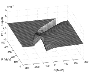
Quasi-particle scheme

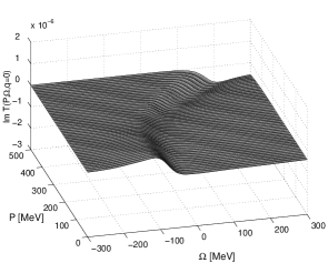
Full scheme

Figure 2: Comparison between the quasi-particle approach (left panel) and our full scheme (right panel) on the level of the $T$-matrix. The dependence upon the center of mass momentum $P$ and the pair energy $\Omega$ is displayed. The relative pair momentum $q$ is set to zero. The chemical potential is $\mu=-40\,\mbox{MeV}$ and the temperature is chosen to be $T=10\,\mbox{MeV}$.

We have applied the CDBONN potential cdb in our calculations. All partial waves up to $J=2$ are included in the sum in eq. (21). Higher partial waves do not contribute significantly to the off-shell structure of $\Sigma$. In contrast, the Hartree-Fock self energy includes partial waves up to $J=9$. In Fig. 2, the thermodynamic $T$ matrix in the quasi-particle scheme, i.e., using a quasi-particle $g^{0}_{\mathrm{II}}$ in eq. (20), is compared to the shape of the full $T$ matrix for zero relative momentum of the nucleon pair. For pair energies $\Omega<2\epsilon(P)$, the $T$ matrix has no imaginary part in the quasi-particle approach. This becomes obvious if one looks at the quasi-particle approximation to $g^{0}_{\mathrm{II}}$,

$$g^{0}_{\mathrm{II}\,QP}(P,\Omega+{\mathrm{i}}\eta,q)=\frac{\left<1-f(\epsilon(k_{1}))-f(\epsilon(k_{2}))\right>_{\theta}}{\Omega-\left<\epsilon(k_{1})+\epsilon(k_{2})\right>_{\theta}+{\mathrm{i}}\eta}.$$ (26)

An imaginary part in the quasi-particle $T$ matrix can only be formed if expression (26) has a pole. For a nucleon pair with zero relative momentum, the sum of the single-particle energies in the denominator yields $2\epsilon(P)$. This leads to a sharp structure in the imaginary part of the $T$ matrix in the quasi-particle approximation for $\Omega\geq 2\epsilon(P)$. This structure is completely smeared out in the full $T$ matrix calculation. In this case ${\mathrm{Im}}T$ is not vanishing also for large negative energies values of $\Omega$.

Once the $T$ matrix is obtained on the $(P,\Omega,q)$-mesh, a three-dimensional interpolation has to be applied in order to carry out the transformation to the integration variables, ($|{\mathbf{k}}^{\prime}|$, $\theta^{\prime}$ and $\omega^{\prime})$, of the energy-momentum integrals in eq. (14). After the evaluation of the real part of the self-energy with the principal value integral in eq. (9), we interpolate the smooth functions ${\mathrm{Re}}\Sigma(k,\omega)$ and ${\mathrm{Im}}\Sigma(k,\omega)$ rather than the spectral function $A(k,\omega)$ to calculate ${\mathrm{Im}}\,g^{0}_{\mathrm{II}}$. The careful evaluation of the integral (19) is one of the crucial steps of the self-consistent procedure. We actually consider

$${\mathrm{Im}}\,g^{0}_{\mathrm{II}}(k_{1},k_{2},\tilde{\Omega}+{\mathrm{i}}\eta)=-\pi\int_{-\infty}^{+\infty}\frac{{\mathrm{d}}\omega}{2\pi}A(k_{1},\omega+\epsilon(k_{1}))A(k_{2},\tilde{\Omega}-\epsilon(k_{1})-\omega)[1-f(\omega+\epsilon(k_{1}))-f(\tilde{\Omega}-\epsilon(k_{1})-\omega)],$$ (27)

where $\tilde{\Omega}=\Omega+\epsilon(k_{1})+\epsilon(k_{2})$. $\epsilon(k)$ is the on-shell energy, which is defined in the same way as the quasi-particle energy, eq. (25). Note that the peaks of the spectral functions in eq. (27) are located around $\omega=0$ and $\omega=\Omega$, independent of $k_{1}$ and $k_{2}$. This simplifies the construction of the integration mesh. Additionally, in the subsequent angle-averaging procedure, we can take advantage of the fact that ${\mathrm{Im}}\,g^{0}_{\mathrm{II}}(k_{1},k_{2},\tilde{\Omega})$ is always peaked around $\Omega=0$.

A sum rule for the two-particle spectral function was given in Ref. dickhoff99 for zero temperature. For the present case, this sum rule can be generalized to

$$-\frac{1}{\pi}\int_{-\infty}^{+\infty}\frac{{\mathrm{d}}\Omega}{2\pi}\,{\mathrm{Im}}\,g^{0}_{\mathrm{II}}(k_{1},k_{2},\Omega+{\mathrm{i}}\eta)=1-n(k_{1})-n(k_{2}).$$ (28)

This relation was used to check the numerical accuracy that was achieved for ${\mathrm{Im}}\,g^{0}_{\mathrm{II}}$ after performing the integration in eq. (19). Mesh spacings and integration limits were adjusted such that both sides of eq. (28) do not deviate by more than $1\%$ for single particle momenta up to $k=3000\,\mbox{MeV}$.

After 6-10 iteration cycles, a self-consistent spectral function $A(k,\omega)$ is obtained. We have performed calculations for a range of chemical potentials between $\mu=-24\,\mbox{MeV}$ and $\mu=5\,\mbox{MeV}$ at $T=10\,\mbox{MeV}$ and for a range of temperatures between $T=5\,\mbox{MeV}$ and $T=20\,\mbox{MeV}$ at $\mu=-15\,\mbox{MeV}$. We found that it is difficult to perform stable and converging calculations below $T=5\,\mbox{MeV}$ in our scheme. The reason for these difficulties is that the number of interpolation and integration mesh points has to be increased strongly in order to obtain stable results. The spectral functions for lower temperatures exhibit structures which require a treatment with a larger number of meshpoints.

To extract information for temperatures below $T=5\,\mbox{MeV}$, we have extrapolated the retarded self-energy to lower temperatures, using the results of five stable calculations at $T=5,7,10,15$ and $20\,\mbox{MeV}$. With the extrapolated self-energy, we have calculated the spectral function at temperatures below $T=5\,\mbox{MeV}$. The reliability of this extrapolation to lower temperatures will be discussed below.

For the range of densities and temperatures we considered, we have found no signals of a pairing instability in the full calculation. The signature of this pairing instability would be a pole in the $T$ matrix at $\Omega=2\mu$ and zero total momentum of the nucleon pair, $P=0$ kadanoff . Although the pole appears on the real $\Omega$ axis only at the critical temperature, $T_{C}$, the formation of the pole structure can be observed already at higher temperatures as a precursor effect alm95 . Inspecting Fig. 2 we can see this precursor structure in the quasi-particle $T$ matrix for $P=0$. This structure is significantly reduced in the full $T$ matrix. The depletion of the Fermi sea due to short-range correlations, in addition to the temperature-induced reduction of occupation at the Fermi surface, weakens the pairing correlations and no indications for a transition to superfluidity are found for the explored range of temperatures. Of course, we cannot exclude such a transition for lower temperatures and/or lower densities.

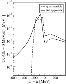
Figure 3: Spectral functions for nucleons with momentum $k=0$ at a temperature $T=10\,\mbox{MeV}$. The spectral function of the self-consistent calculation (solid line) has been determined for $\mu=-15\,\mbox{MeV}$, which corresponds to a density of $\rho=0.36\,\mbox{fm}^{-3}$. The results for the quasi-particle approximation (dashed line) are taken from a calculation at $\rho=0.3\,\mbox{fm}^{-3}$.

Characteristic differences between the quasi-particle approximation and the full $T$-matrix approach can also be seen in Fig 3, which shows a comparison of the spectral functions for nucleons with momentum $k=0$ in nuclear matter of a density $\rho$ around 0.3 fm^-3 at temperature $T$ = 10 MeV. While the quasi-particle spectral function tends to zero below $\omega-\mu=200\,\mbox{MeV}$, the self-consistent result shows a large tail at negative energies. This redistribution of strength is related to the tail that was found in the imaginary part of the full $T$ matrix in Fig 2. In the full calculation one does not constrain e.g. the construction of the self-energy at energies below the Fermi energy to the admixture of two-hole one-particle configurations, as it is done in the quasi-particle approach, but the self-consistent evaluation allows for general n-hole (n-1)-particle configurations. The double-hump structure in the quasi-particle spectral function reflects the fact that, for low lying states, eq. (25) has no unique solution (cf. paragraph after eq. (25)). The self-consistent spectral functions do not show this feature any more. The double hump can be interpreted as an indication for a strong coupling of the one-hole configuration to two-hole one-particle excitations. Obviously this coupling is reduced in the self-consistent calculation.

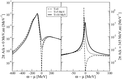
Figure 4: Spectral functions in nuclear matter as a function of the energy at different temperatures. The left panel shows results for $k=0$, while the spectral functions displayed in the right panel have been evaluated for $k=345\,\mbox{MeV}$, a momentum just below the Fermi momentum for the density $\rho=0.36\,\mbox{fm}^{-3}$, which corresponds to $\mu=-15\,\mbox{MeV}$.

Spectral functions for nuclear matter at different temperatures are displayed in Fig. 4 considering a value for $\mu=-15\,\mbox{MeV}$, which corresponds to a density of about 0.36 fm^-3. The left panel presents the spectral function for low-lying hole states with momentum $k=0\,\mbox{MeV}$. Note that the spectral function for $T=0$, which has been obtained by extrapolating the self-energy from self-consistent results evaluated for $T$ larger than 5 MeV, shows the correct behavior and vanishes for $\omega$ equal to $\mu$, separating the hole and particle part of the spectral function. This separation is of course smeared out at finite temperatures. The width of the spectral distribution is large for $k=0$ at all temperatures and almost no broadening effect due to the temperature can be observed. This can also bee seen from Table 1, which lists results for this width.

The spectral function for loosely bound hole states is displayed in the right panel of Fig. 4 assuming a momentum of $k=345\,\mbox{MeV}$, which is just below the Fermi momentum of the density under consideration. In this case the width of the spectral distribution is much smaller than for $k=0$. Note the different energy scale in this part of the figure. With increasing $T$, the peak of the spectral function clearly broadens and it is shifted to higher energies. At $T=10\,\mbox{MeV}$, it is almost symmetric around $\omega=\mu$. This means that at this temperature one does not observe any dip in the spectral function at the energy $\omega=\mu$.

The binding energy per particle, $E/A$ was calculated from the self-consistent spectral function using the Koltun’s sum rule:

$$\frac{E}{A}=\frac{d}{\rho}\int\frac{{\mathrm{d}}^{3}k}{(2\pi)^{3}}\int_{-\infty}^{+\infty}\frac{{\mathrm{d}}\omega}{2\pi}\frac{1}{2}\left(\frac{k^{2}}{2m}+\omega\right)A(k,\omega)f(\omega),$$ (29)

where $d=4$ is the spin-isospin degeneracy factor for symmetric nuclear matter. A corresponding integral can be used to determine the kinetic energy per nucleon, $E_{kin}/A$, which implies that we can also evaluate the potential energy $E_{pot}/A$. The density $\rho$ of the system is given by

$$\rho=d\int\frac{{\mathrm{d}}^{3}k}{(2\pi)^{3}}n(k)=\frac{d}{6\pi^{2}}\left(k^{*}\right)^{3}\,.$$ (30)

Both energy and density converged to a high degree of accuracy of typically better than $0.1\%$ by the end of the iteration. The temperature dependence of some energy observables is given in Table 1. All values at $T=5\,\mbox{MeV}$ and above were obtained from eq. (29) using self-consistent spectral functions. The values at $T=4\,\mbox{MeV}$ and $T=3\,\mbox{MeV}$ were calculated from the self-consistent results at $T$ larger and equal to 5 MeV, extrapolating the results for the self-energies. The self-energy is a rather smooth function, but of course the extrapolation introduces uncertainties. We estimate an error up to about $3\%$ for the interpolated values. In order to test this interpolation, we have also evaluated the total energy per nucleon for those temperatures, for which a self-consistent result exists, by interpolation from the remaining temperatures. These energies are listed in the column of Table 1, which is labeled $E/A_{\mbox{ext}.}$

At low $T$, we found an almost perfect quadratic dependence between the binding energy $E/A$ and the temperature. From this dependence we extrapolate the total energy per nucleon at zero temperature to -17.9 MeV . The decrease of binding with increasing $T$ is mainly, but not only, due to an increase of the kinetic energy.

In the last two columns of Table 1, we present the on-shell width $\Gamma(k,\epsilon(k))$ at $k=0$ and at a momentum close to the Fermi surface. While this width is almost independent on the temperature for the low-lying states ($k=0$), it increases strongly with $T$ for the states close to the Fermi surface with a momentum ($k=k^{*}$, see eq.(30)).

The density dependence of the spectral width is shown in Table 2. The density of the system and the Fermi momentum $k^{*}$ of a filled sphere corresponding to that density are also reported. While the on-shell width for $k=0$ increases with density, the width at $k=k^{*}$ decreases. As we have seen already in Table 1, the width for the low-lying states is mainly determined by the phase space of the occupied states, which does not depend on the temperature, but on the density. In contrary, at the Fermi surface, the width is determined by the temperature deformation of the Fermi surface. Since this deformation is more drastic at lower densities, the width there is larger.

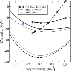
Figure 5: Binding energy per nucleon (solid lines) and the chemical potential (dashed lines) in symmetric nuclear matter as a function of the density $\rho$. Results of a full Green’s function calculation at a temperature $T=10\,\mbox{MeV}$ (squares connected by a line), are compared to BHF results are shown for zero temperature (thin lines) and $T=10\,\mbox{MeV}$ (thick lines). The large square represents the ‘empirical’ saturation region that can be derived from the Bethe-Weizsäcker formula.

In Fig. 5, the binding energy per particle $E/A$ (solid line with squares) and the chemical potential $\mu$ (dashed line with squares) are plotted versus the density of the system at $T=10\,\mbox{MeV}$. For a comparison we also present corresponding results of BHF calculations (continuous choice for the single-particle spectrum) for $T=10\,\mbox{MeV}$ (thick lines) and for zero temperature (thin lines). We find a repulsive effect in the full $T$ matrix calculation compared to the BHF calculation at the same temperature. This repulsive effect increases with density, therefore the saturation density obtained in the full $T$-matrix calculation is smaller than the one obtained in the BHF approach. The resulting density, $\rho_{sat}=0.31\,\mbox{fm}^{-3}$, however, is still almost twice as large as the ‘empirical value’, $\rho_{0}=0.16\,\mbox{fm}^{-3}$. This repulsive effect relative to the BHF calculations is consistent with the observations of Ref. bozek01 , both with respect to the density dependence but also with respect to the size of the repulsion.

The so-called Hugenholtz-Van Hove theorem states that, at zero temperature, the chemical potential should be equal to the binding energy at the saturation point hugenholtz . The theorem is clearly violated by about $20\,\mbox{MeV}$ in the BHF approach, while it should be fulfilled in the self-consistent $T$ matrix approach. This was first shown to be the case by Bożek and Czerski for a self-consistent $T$ matrix approach using separable potentials bozek01 . Although a zero temperature treatment is not really feasible in our approach, we can conclude a reasonable thermodynamic consistency in our calculation from the fact that the intersection point of $\mu(\rho)$ with the binding curve at $T=10\,\mbox{MeV}$ is located slightly above the saturation density. While the binding energy will increase as $T$ approaches zero, the chemical potential will become less attractive for a given density, such that the intersection point moves closer to the expected region.

IV Conclusions

In this paper, we have presented a method for a self-consistent evaluation of the one- and two-body Greens function of nuclear matter in the ladder approximation. In contrast to previous works, no parameterizations of the single-particle spectral functions were used and and the full structure of a realistic NN interaction (CDBONN) was taken into account. This requires evaluation of the in-medium NN $T$ matrix, the self-energy and the spectral functions of the nucleons for a wide range of energies and momenta. The equations describing these quantities were solved in an iterative scheme, for a given temperature and chemical potential. Self-consistency could be established after several iterations so that calculation of observables from these Greens functions converged to a high degree of accuracy.

This computational scheme works rather well for temperatures above $T$ = 5 MeV. The spectral functions for lower temperatures exhibit sharp structures, which requires a large number of meshpoints for a reliable representation. This inhibits direct calculations at very low temperatures. Therefore we introduce an extrapolation procedure, which is based on the smooth behavior of the nucleon self-energy, to deduce results also for lower temperatures.

For the range of densities and temperatures we considered, no signals of a pairing instability have been observed in the full calculation. The distribution of strength in the self-consistent spectral function shields the system against this instability, which is observed in the quasi-particle approximation. This supports the findings of investigations using separable NN interactions or parameterizations of the spectral distributionddnsw ; bozek01 .

Comparing the total energies per nucleon calculated with the self-consistent $T$-matrix approach with the corresponding results obtained in BHF calculations we observe a repulsive effect of around 5 MeV per nucleon. As this repulsion increases with density, the saturation density of the self-consistent Greens function calculation is shifted to lower densities. The resulting saturation density, however, is still too large as compared to the empirical value.

The consistent treatment of hole-hole and particle-particle scattering terms in the full $T$-matrix calculation leads to results, which are consistent from the thermodynamic point of view. Therefore, the Hugenholtz-Van Hove theorem, which is violated in the BHF approach, is respected in the Self-consistent Greens function approach (see also bozek01 ).

We would like to acknowledge financial support from the Europäische Graduiertenkolleg Tübingen - Basel (DFG - SNF).

$T$ [MeV]	$E/A$ [MeV]	$E/A_{\mbox{ext}.}$ [MeV]	$E_{kin}/A$ [MeV]	$E_{pot}/A$ [MeV]	$\Gamma(0,\epsilon(0))$ [MeV]	$\Gamma(k^{*},\epsilon(k^{*}))$ [MeV]
20	-7.05	-6.3	58.41	-65.46	59.2	15.5
15	-11.14	-11.3	54.45	-65.61	58.2	9.3
10	-14.53	-14.7	52.48	-67.01	58.4	4.7
7	-16.32	-16.2	51.87	-68.17	60.5	2.5
5	-17.0	-17.1	50.9	-67.9	62.6	1.5
4	-	-17.4	50.9	-68.3	-	-
3	-	-17.6	51.0	-68.6	-	-

Table 1: Energy, $E/A$, kinetic Energy, $E_{kin}/A$, and potential energy per nucleon, $E_{pot}/A$, calculated for symmetric nuclear matter for a chemical potential $\mu=-15\,\mbox{MeV}$, which corresponds to a density of $\rho=0.36\,\mbox{fm}^{-3}$, at different temperatures $T$. The values at $T=4\,\mbox{MeV}$ and $T=3\,\mbox{MeV}$ were obtained from an extrapolation of the self-energies evaluated at higher temperatures. Also displayed are the values for the on-shell width of the self-energy of nucleons with momentum $k=0$ and $k=k^{*}=340$ MeV (see eq.(30)).

$\mu$ [MeV]	$\rho$ [$\mbox{fm}^{-3}$]	$k^{*}$ [MeV]	$\Gamma(0,\epsilon(0))$ [MeV]	$\Gamma(k^{*},\epsilon(k^{*}))$ [MeV]
-23	0.254	307	48.9	6.7
-20	0.306	326	53.3	5.5
-15	0.364	345	58.4	4.7
-5	0.44	368	63.0	3.5
5	0.51	385	70.1	3.7

Table 2: Density-dependence of the on-shell width for $k=0$ and the momentum $k^{*}$ (see eq.(30)). The density is reported for each chemical potential, too. All calculations were performed at $T=10\,\mbox{MeV}$.

References

- (1) M. Baldo, Nuclear methods and the Nuclear Equation of State, Int. Rev. of Nucl. Physics, Vol. 9 (World-Scientific, Singapore, 1999)
- (2) H. Müther and A. Polls, Prog. in Part. and Nucl. Phys. 45, 243 (2000)
- (3) I. Sick and P.K.A. deWitt Huberts, Comm. Nucl. Part. Phys. 20, 177 (1991)
- (4) M.F. van Batenburg, Ph.D. Thesis, University of Utrecht (2001).
- (5) A. Ramos, A. Polls, and W.H. Dickhoff, Nucl. Phys. A 503, 1 (1989)
- (6) O. Benhar, A. Fabrocini, and S. Fantoni, Nucl. Phys. A 505, 267 (1989)
- (7) H. Müther, G. Knehr, and A. Polls, Phys. Rev. C 52, 2955 (1995)
- (8) B.E. Vonderfecht, W.H. Dickhoff, A. Polls, and A. Ramos, Phys. Rev. C 44, R1265 (1991)
- (9) K. Amir-Azimi-Nili, H. Müther, L.D. Skouras, and A.Polls, Nucl. Phys. A 604, 245 (1996)
- (10) B.D. Day, Rev. Mod. Phys. 39, 719 (1967)
- (11) A. Akmal and V.R. Pandharipande, Phys. Rev. C 56, 2261 (1997)
- (12) S. Fantoni and A. Fabrocini in Microscopic Quantum Many-Body Theories and Their Applications, eds. J. Navaroo and A. Polls (Springer 1998)
- (13) L. P. Kadanoff and G. Baym, Quantum Statistical Mechanics (Benjamin, New York, 1962)
- (14) W. D. Kraeft, D. Kremp, W. Ebeling and G. Röpke, Quantum Statistics of Charged Particle Systems (Akademie-Verlag, Berlin, 1986)
- (15) H.S. Köhler, Phys. Rev. C 46, 1687 (1992)
- (16) H.S. Köhler and R. Malfliet, Phys. Rev. C 48, 1034 (1993)
- (17) T. Frick, Kh. Gad, H. Müther, and P. Czerski, Phys. Rev. C 65, 34321 (2002)
- (18) B.E. Vonderfecht, W.H. Dickhoff, A. Polls, and A. Ramos, Nucl. Phys. A 555, 1 (1993)
- (19) T. Alm, G. Röpke, A. Schnell, N.H. Kwong, and H.S. Köhler, Phys. Rev. C 53, 2181 (1996)
- (20) P. Bożek, Nucl. Phys. A 657, 187 (1999)
- (21) M. Baldo, I. Bombaci, and U. Lombardo, Phys. Lett. B 283, 8 (1992)
- (22) T. Alm, B. L. Friman, G. Röpke and H. Schulz, Nucl. Phys. A 551, 45 (1993)
- (23) Ø. Elgarøy, L. Engvik, E. Osnes, and M. Hjorth-Jensen, Phys. Rev. C 57, R1069 (1998)
- (24) Y. Dewulf, D. Van Neck, and M. Waroquier, Phys. Rev. C 65, 054316 (2002)
- (25) E.P. Roth, Ph.D. Thesis, University of St. Louis (2000), W.H. Dickhoff and E.P. Roth, Acta Phys. Pol. B 33, 65 (2002)
- (26) Y. Dewulf, W.H. Dickhoff, D. Van Neck, E.R. Stoddard, and M. Waroquier, Phys. Rev. Lett. 90, 2003 (152501)
- (27) P. Bożek and P. Czerski, Eur. Phys. J. A 11, 271 (2001)
- (28) P. Bożek, Phys. Rev. C 65, 054306 (2002)
- (29) P. Bożek, Eur. Phys. J. A 15, 325 (2002)
- (30) E. Heinz, H. Müther, and H.A. Mavromatis, Nucl. Phys. A 587, 77 (1995)
- (31) R. Machleidt, F. Sammarruca, and Y. Song, Phys. Rev. C 53, R1483 (1996)
- (32) A. Schnell, Ph.D. Thesis, University of Rostock (1996)
- (33) P. Bożek, Phys. Rev. C 59, 2619 (1999)
- (34) Y. Dewulf, Ph.D. Thesis, University of Gent (2000)
- (35) C. Bloch and C. De Dominicis, Nucl. Phys. 7, 459 (1958)
- (36) M.I. Haftel and F. Tabakin, Nucl. Phys. A 158, 1 (1970)
- (37) W.H. Dickhoff, C.C. Gearhart, E.P. Roth, A. Polls and A. Ramos, Phys. Rev. C 60, 064319 (1999)
- (38) N.M. Hugenholtz and L. Van Hove, Physica 24, 363 (1958)