Simple solutions of relativistic hydrodynamics
for longitudinally and cylindrically expanding systems

Abstract

Simple, self-similar, analytic solutions of 1 + 1 dimensional relativistic hydrodynamics are presented, generalizing the Hwa - Bjorken boost-invariant solution to inhomogeneous rapidity distributions. These solutions are generalized also to 1 + 3 dimensional, cylindrically symmetric firetubes, corresponding to central collisions of heavy ions at relativistic bombarding energies.

1 Introduction

Analytic solution of the equations of relativistic hydrodynamics is a difficult task because the equations are non-linear partial differential equations, that are rather complicated to handle not only analytically but also numerically. However, relativistic hydrodynamics has various applications, including the calculations of single-particle spectra and two-particle correlations in relativistic heavy ion collisions, see ref [1]. More recently, there has been an increasing interest in applications of relativistic hydrodynamics in Au+Au collisions at RHIC both at $\sqrt{s}=130$ AGeV and $\sqrt{s}=200$AGeV bombarding energies, predictions were made for the coming LHC experiments [2, 3, 4]. The hydrodynamical analysis can also be extended to the study of these processes on event-by-event basis [5, 6]. However, most works in hydrodynamics are numerical so not always transparent.

In this sense, exact solutions would be useful, but are rarely found due to the highly non-linear nature of relativistic hydrodynamics. Khalatnikov’s one-dimensional analytical solution [7] to Landau’s hydrodynamic model [8] gave rise to a new approach in high energy physics. The boost-invariant solution [9] was found later by R. C. Hwa and other authors. It has been frequently utilized as the basis for estimations of initial energy densities in ultra-relativistic nucleus-nucleus collisions[10]. Due to this famous application this boost-invariant solution is frequently called as Bjorken’s solution, although as far as we know it was first described by R. Hwa in ref. [9]. Perhaps it should be called the Hwa-Bjorken solution, which name we shall use hereafter.

Recently, Biró has found self-similar exact solutions of relativistic hydrodynamics for cylindrically expanding systems [11, 12]. However, his solutions are valid only when the pressure is independent of space and time, as e.g. in the case of a rehadronization phase transition in the middle of a relativistic heavy ion collision.

Here we present an analytic approach, which goes back to the data-motivated exact analytic solution of non-relativistic hydrodynamics found by Zimányi, Bondorf and Garpman (ZBG) in 1978 for low energy heavy ion collisions with spherical symmetry [13]. This solution has been extended to the case of elliptic symmetry by Zimányi and collaborators in ref. [14]. In  [15, 16] a Gaussian parameterization has been introduced to describe the mass dependence of the effective temperature and the radius parameters of the two-particle Bose-Einstein correlation functions in high energy heavy ion collisions. Later it has been realized that this phenomenological parameterization of data corresponds to an exact, Gaussian solution of non-relativistic hydrodynamics with spherical symmetry [17]. The spherically symmetric self-similar solutions of non-relativistic hydrodynamics were obtained in a general manner in [18], that included an arbitrary scaling function for the temperature profile, and expressed the density distribution in terms of the temperature profile function. The ZBG solution and the Gaussian solution of [17] are recovered from the general solution of  [18] as special cases, corresponding to different scaling functions of the temperature profile. The Gaussian solution has been generalized to ellipsoidal expansions in [19], that provides analytic insight into the physics of non-central heavy ion collisions [20].

Our approach corresponds to a generalization of these recently obtained analytic solutions [17, 18, 20, 21] of non-relativistic fireball hydrodynamics to the case of relativistic longitudinal and transverse flows. In particular, an analytic approach, the Buda-Lund (BL) model has been developed to parameterize the single particle spectra and the two-particle Bose-Einstein correlations in high-energy heavy-ion physics in terms of hydrodynamically expanding, cylindrically symmetric sources [22]. Here we attempt to find a family of exact solutions of relativistic hydrodynamics that may include the BL model as a particular limiting case. It turns out that in the simplest case our result corresponds to the Cracow hydrodynamic parametization, which is successfull in describing single particle spectra of Au+Au collisions at $\sqrt{s}=130$ and 200 AGeV at RHIC[23, 24, 25].

2 The equations of relativistic hydrodynamics

We solve the relativistic continuity and energy-momentum conservation equation:

$$\partial_{\mu}(nu^{\mu}) = 0\,,$$ (1)

$$\partial_{\nu}T^{\mu\nu} = 0\,.$$ (2)

Here $n\equiv n(t,{\mathbf{r}})$ is the number density, the four-velocity is denoted by $u^{\mu}\equiv u^{\mu}(t,{\mathbf{r}})=\gamma(1,{\mathbf{v}})$, normalized to $u^{\mu}u_{\mu}=\gamma^{2}(1-{\mathbf{v}}^{2})=1$, and the energy-momentum tensor is denoted by $T^{\mu\nu}$. We assume perfect fluid,

$$T^{\mu\nu}=(\epsilon+p)u^{\mu}u^{\nu}-pg^{\mu\nu},$$ (3)

where $\epsilon$ stands for the relativistic energy density and $p$ denotes the pressure.

We close this set of relativistic hydrodynamical equations with the equations of state. We assume a gas containing massive conserved quanta,

$$\epsilon = mn+\kappa p\,,$$ (4)

$$p = nT.$$ (5)

The equations of state have two free parameters, $m$ and $\kappa$. Non-relativistic hydrodynamics of ideal gases corresponds to the limiting case of $m\gg T$, ${\mathbf{v}}^{2}\ll 1$ and $\kappa=3/2\,$. Relativistic hydrodynamics for massless particles and a constant speed of sound $c_{s}^{2}$ corresponds to the case of $m=0$ and $c_{s}^{2}=1/\kappa$.

The energy-momentum conservation equations can be projected into a component parallel to $u^{\mu}$ and components orthogonal to $u^{\mu}$, which are respectively the relativistic energy and Euler equations:

$$u^{\mu}\partial_{\mu}\epsilon+(\epsilon+p)\partial_{\mu}u^{\mu} = 0\,,$$ (6)

$$u_{\nu}u^{\mu}\partial_{\mu}p+(\epsilon+p)u^{\mu}\partial_{\mu}u_{\nu}-\partial_{\nu}p = 0\,.$$ (7)

Based on general thermodynamical considerations, one can show that the expansion is adiabatic:

$$\partial_{\mu}(\sigma u^{\mu})=0\,,$$ (8)

where $\sigma$ is the entrophy density. This relation holds for perfect fluids, independently of the equations of state.

With the help of the equations of state and the continuity equation, the energy equation can be rewritten as an equation for the temperature,

$$u^{\mu}\partial_{\mu}T+\frac{1}{\kappa}T\partial_{\mu}u^{\mu}=0\,.$$ (9)

We solve 5 independent equations, the continuity, the (3 spatial components of) relativistic Euler, and the temperature equation, eqs. (1,7,9). The equations of state, eq. (4,5) close this system of equations in terms of 5 variables, $n$, $T$ and ${\mathbf{v}}=(v_{x},v_{y},v_{z})$.

3 Self-similarity

We look for solutions which generalize the usual similarity flow, in which the flow pattern is unchanged with time if the scales of length $X(t),Y(t),Z(t)$ along three orthogonal directions vary appropriately, namely, we consider

$${\mathbf{v}}=\left(\frac{\dot{X}(t)}{X(t)}r_{x},\frac{\dot{Y}(t)}{Y(t)}r_{y},\frac{\dot{Z}(t)}{Z(t)}r_{z}\right)\,,$$ (10)

where $x^{\mu}\equiv(t,r_{x}\,,r_{y}\,,r_{z})$ and the dot indicates the time derivative. As for the thermodynamic quantities such as $n(x^{\mu}),T(x^{\mu}),p(x^{\mu}),\ldots,$ we search solutions of the form

$$f(x^{\mu})=f_{0}\left(\frac{V_{0}}{V}\right)^{a}F(s)\,,$$ (11)

where the volume parameter $V=XYZ$, $a$ is an appropriate exponent and $F(s)$ is an arbitrary fuction of the scaling variable defined by

$$s=\frac{r_{x}^{2}}{X^{2}}+\frac{r_{y}^{2}}{Y^{2}}+\frac{r_{z}^{2}}{Z^{2}}\ .$$ (12)

These are Hubble type of flows, but the thermodynamic quantities may contain arbitrary functions depending on the the scale parameter $s$ and also, at least in principle, the scale parameters $X(t),Y(t)$ and $Z(t)$ may be different in the principal directions. Their derivatives, $\dot{X}(t)$, $\dot{Y}(t)$ and $\dot{Z}(t)$ correspond to (direction and time dependent, generalized) Hubble constants.

In heavy-ion collisions, the well known boost-invariant solution [9] is often utilized to discuss several properties of data. However, this solution has some shortcomings: i) it is scale invariant, having a flat rapidity distribution, corresponding to the extreme relativistic collisions; ii) it contains no transverse flow. In the present paper, we apply the strategy described above first to 1+1 dimensional (time + longitudinal coordinate) case and obtain a class of solutions which are able to describe inhomogeneous rapidity distributions, overcoming the first shortcoming mentioned above. Then, in section 5, we consider the case of cylindrically symmetric case, trying to overcome the second shortcoming.

4 Simple 1+1 dimensional solutions

In this section, we solve the 1+1 dimensional problem. Hence $x^{\mu}=(t,r_{z})$, $k^{\mu}=(E,k_{z})$ throughout this section. The metric tensor is $g^{\mu\nu}=g_{\mu\nu}=\mbox{\rm diag}(1,-1)$ and $x_{\mu}=(t,-r_{z})$. We solve 3 independent equations, the continuity, the temperature equation and the $z$ component of the Euler equation (1,7,9). The equations, (4,5) close this system of equations in terms of 3 variables, $n$, $T$ and $v_{z}$.

We look for flows that scale in the $z$ direction. The scaling variable, eq.(12), in this case is defined as

$$s=\frac{r_{z}^{2}}{Z\left(t\right)^{2}},$$ (13)

and the longitudinal velocity

$$v_{z}(t,r_{z})=\frac{\dot{Z}(t)}{Z(t)}r_{z},$$ (14)

where $\dot{Z}=dZ(t)/dt\,$. In the relativistic notation, this form is equivalent to

$$u^{\mu} = (\cosh\zeta,\sinh\zeta),$$ (15)

$$\tanh\zeta = \frac{\dot{Z}(t)}{Z(t)}r_{z},\qquad\mbox{\rm or}\quad\cosh\zeta\,=\,\frac{1}{\sqrt{1-\dot{Z}^{2}s}}\equiv\gamma.$$ (16)

Note that from eq. (16) it is obvious that this solution can be defined only in a bounded longitudinal coordinate region, because at any time $|r_{z}|\leq Z(t)/\dot{Z}(t)$ has to be satisfied. Using this ansatz, we find that the continuity equation is solved by the form

$$n(t,r_{z})=n_{0}\frac{Z_{0}}{Z}\frac{1}{\cosh\zeta}\mathcal{G}(s),$$ (17)

where $\mathcal{G}(s)$ is an arbitrary non-negative function of the scaling variable $s$ and $n_{0}$ and $Z_{0}$ are normalization constants. We use the convention $Z_{0}=Z(t_{0})$ and $n_{0}=n(t_{0},0)$ which implies that $\mathcal{G}(s=0)=1$. The temperature equation, (9) is solved by the following form:

$$T(t,r_{z})=T_{0}\left(\frac{Z_{0}}{Z}\frac{1}{\cosh\zeta}\right)^{1/\kappa}\mathcal{F}(s).$$ (18)

The constants of normalization are chosen such that $T_{0}=T(t_{0},0)$ and $\mathcal{F}(0)=1$. Here again, we find that the solution is independent of the form of the function $\mathcal{F}(s)$. From the positivity of the temperature distribution it follows that $\mathcal{F}(s)\geq 0$.

Using the ansatz for the flow profile and the solution for the density and the temperature, the relativistic Euler equation reduces to a complicated non-linear equation that contains $Z$, $\dot{Z}$ and $\ddot{Z}$ and $s$. Taking this equation at $s=0$ we express $\ddot{Z}$ as a function of $Z$ and $\dot{Z}$. Substituting this back to the Euler equation we obtain an equation for $\dot{Z},Z$ and $s$. In particular, for the $m=0$ case, $Z$ cancels out and this reduces to a second order polynomial equation for $\dot{Z}^{2}$, which has only one positive root. The form of the solution in this case ($m=0$) is $\dot{Z}^{2}(t)=F(s)$. Observing that the function $F$ depends only on the scaling variable $s$, while $\dot{Z}$ depends only on the time variable $t$, we conclude that the only solution of this equation should be a constant $\dot{Z}=\dot{Z}_{0}$. Now we choose the origin of the time axis such that $Z(t=0)=0$ without loss of generality. The solutions can be cast in a relatively simple form by introducing the longitudinal proper time $\tau$ and the space-time rapidity $\eta$,

$$\tau = \sqrt{t^{2}-r_{z}^{2}},$$ (19)

$$\eta = \frac{1}{2}\log\left(\frac{t+r_{z}}{t-r_{z}}\right).$$ (20)

This implies that $Z(t)=\dot{Z}_{0}t$, $v_{z}=\frac{r_{z}}{t}=\tanh\eta$ and $\zeta=\eta$. Thus the solution for the flow velocity field corresponds to the flow field of the boost-invariant solution. However, in the boost-invariant solution the temperature distribution was independent of the $\eta$ variable, while in our case the density and the temperature distributions can be both $\eta$ dependent, or in other words, our solutions are scale dependent. The scale is defined by the parameter $\dot{Z}_{0}$, in the longitudinal direction.

This special form of the solution for the flow velocity field implies that $\ddot{Z}=0$. This equation implies that there is no pressure gradient and there is no acceleration in this class of self-similar solutions, similarly to the case of boost-invariant solution. The Euler equation is reduced to the following requirement:

$$(\partial_{z}+\frac{r_{z}}{t}\partial_{t})\left[\left(\frac{t_{0}}{\tau}\right)^{(1+1/\kappa)}(1-\dot{Z}_{0}^{2}s)^{(1+1/\kappa)}\mathcal{G}(s)\mathcal{F}(s)\right]=0$$ (21)

This equation is solved by the trivial $\mathcal{G}(s)\mathcal{F}(s)=0$ as well as by the non-trivial solution of

$$\mathcal{G}(s)\mathcal{F}(s)=(1-\dot{Z}_{0}^{2}s)^{-(1+1/\kappa)},$$ (22)

which is indeed only a function of $s$ as $\dot{Z}_{0}$ is a constant of time. With this form, the Euler equation is satisfied. This solution implies that the scaling profile functions for the temperature and the density distribution are not independent. As the constraint is given only for their product, one of them can be still chosen in an arbitrary manner.

It is worthwhile to introduce new forms of the scaling functions. Let us define

$$\mathcal{T}(s) = \mathcal{F}(s)(1-\dot{Z}_{0}^{2}s)^{1/\kappa},$$ (23)

$$\mathcal{V}(s) = \mathcal{G}(s)(1-\dot{Z}_{0}^{2}s)\,.$$ (24)

Then the constraint Eq. (22) can be cast to the simplest form of

$$\mathcal{V}(s)\mathcal{T}(s)=1.$$ (25)

Let us summarize our new family of solutions of the 1+1 dimensional relativistic hydrodynamics by substituting the results in the density, temperature and pressure profiles. We obtain

$$v_{z} = \frac{r_{z}}{t}=\tanh\eta,$$ (26)

$$s = \frac{r_{z}^{2}}{\dot{Z}_{0}^{2}t^{2}}\,=\,\frac{\tanh^{2}\eta}{\dot{Z}_{0}^{2}},$$ (27)

$$n = n_{0}\frac{t_{0}}{\tau}\mathcal{V}(s),$$ (28)

$$p = p_{0}\left(\frac{t_{0}}{\tau}\right)^{1+1/\kappa},$$ (29)

$$T = T_{0}\left(\frac{t_{0}}{\tau}\right)^{1/\kappa}\frac{1}{\mathcal{V}(s)},$$ (30)

where $p_{0}=n_{0}T_{0}$. Thus we have generated a new family of exact solutions of relativistic hydrodynamics: a new hydrodynamical solution is assigned to each non-negative function $\mathcal{V}(s)$. It can be checked that the above solutions are valid also for massive particles, the form of the solution is independent of the value of the mass $m$. The form of solutions depends parametrically on $\kappa$, that characterizes the equation of state.

4.1 Analysis of the solutions

The pressure and the flow profiles of the above 1+1 dimensional relativistic hydro solution are the same as in the boost-invariant solution. In the case of $\mathcal{V}(s)=1,$ we recover the Hwa-Bjorken boost-invariant solution of refs. [9, 10]. In this limiting case, the pressure, the density and the temperature profiles depend only on the longitudinal proper time $\tau$.

In the general case, our solution contains a characteristic scale defining parameter in the longitudinal direction, $\dot{Z}_{0}$, and an arbitrary scaling function $\mathcal{V}(s)$. Thus we have an infinitely rich new family of solutions. Let us try to determine the physical meaning of the scaling function $\mathcal{V}(s)$.

In order to do this we evaluate the single particle spectra corresponding to the new solutions. Here we neglect any possible dynamics in the transverse directions, as usual in case of applications of the boost-invariant solution. The four-velocity field of our solutions thus becomes $u^{\mu}=(\cosh\eta,0,0,\sinh\eta)$. The four-momentum of the observed particles with mass $m$ is denoted by $k^{\mu}=(m_{t}\cosh$ $y,k_{x},k_{y},m_{t}\sinh$ $y)$.  Let us assume that particles freeze out at a constant longitudinal proper-time $\tau_{f}$, for the sake of simplicity. This implies freeze-out at a constant pressure, but at a space-time rapidity dependent temperature and density, and makes it possible to continue the calculation analytically. The source function of locally thermalized relativistically flowing particles in a Boltzmann approximation can be written as

$$S(x,\mathbf{k})=C({\eta})\,m_{t}\cosh(\eta-y)\,n(x)\,\exp\left(-k^{\mu}u_{\mu}/T\right)\,\delta(\tau-\tau_{f}),$$ (31)

where $C(\eta)$ is an $\eta$ dependent normalization factor, given by the condition that $\int d\mathbf{k}/E\,S(x,\mathbf{k})=n(x)\delta(\tau-\tau_{f})$, which implies that

$$C(\eta)=\left\{4\pi m^{2}T(\tau_{f},\eta)K_{2}[m/T(\tau_{f},\eta)]\right\}^{-1},$$ (32)

where $K_{\nu}(z)=\int_{0}^{\infty}dz\exp(-z\cosh t)\cosh(\nu t)$ is the modified Bessel function of the second kind.

The single particle spectrum can be calculated from the emission function as

$$E\frac{d^{3}N}{d\mathbf{k}}=\int\tau d\tau d\eta S(x,\mathbf{k}).$$ (33)

Substituting our family of new solutions, and using $\mathcal{T}(x)=1/\mathcal{V}(x)$, we obtain

$$S(x,\mathbf{k}) = \,C(\eta)\,m_{t}\cosh(\eta-y)\,n(x)f_{B}(x,\mathbf{k})$$ (34)

$$f_{B}(x,\mathbf{k}) = \exp\left[{-\frac{m_{t}\cosh(\eta-y)}{T_{0}}}\left({\frac{\tau}{t_{0}}}\right)^{1/\kappa}{\mathcal{V}(\frac{\tanh^{2}\eta}{\dot{Z}_{0}^{2}})}\right]\delta(\tau-\tau_{f}).$$ (35)

We are interested in the coupling between the measurable rapidity distribution and the rapidity dependence of the effective temperature in the transverse directions as obtained from our new family of solutions. We assume that $\mathcal{V}(s)$ is a slowly varying function, i.e. $d\log\mathcal{V}(s)/ds\ll 1$ in the region of interest. This assumption implies that the point of maximal emissivity is located at $\overline{\eta}=y$ with correction terms of $\mathcal{O}(d\log\mathcal{V}(s)/ds)$ The measurable single-particle spectra can be written as

$$E\frac{d^{3}N}{d\mathbf{k}} = 2C(y)\,n_{0}t_{0}\,\mathcal{V}\left(\frac{\tanh^{2}y}{\dot{Z}_{0}^{2}}\right)K_{1}[m_{t}/T_{\mathrm{eff}}\left(y\right)],$$ (36)

$$\frac{dN}{dy} = n_{0}t_{0}\mathcal{V}\left(\frac{\tanh^{2}y}{\dot{Z}_{0}^{2}}\right).$$ (37)

where

$$T_{\mathrm{eff}}(y)=\frac{1}{\mathcal{V}\left(\frac{\tanh^{2}y}{\dot{Z_{0}}^{2}}\right)}T_{0}\left(\frac{t_{0}}{\tau_{f}}\right)^{1/\kappa}.$$ (38)

Note that the $\mathcal{V}$ function is a free fit function that describes the measurable rapidity distribution, including characteristic scales of the size of $\dot{Z}_{0}$.

We see that the slope parameter for transverse mass distribution $T_{\mathrm{eff}}$ is related to the rapidity distribution as

$$T_{\mathrm{eff}}(y)=T_{0}\left(\frac{t_{0}}{\tau_{f}}\right)^{1/\kappa}{\frac{dN/dy\left(y=0\right)}{dN/dy}}.$$ (39)

Figures 1 and 2 illustrate the calculated behavior of the effective temperature distribution as a function of rapidity for a single Gaussian-like and a double Gaussian-like ansatz for the measurable rapidity distribution.

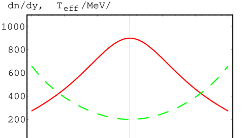
Figure 1: Rapidity distribution $dN/dy$ and effective temperature distribution $T_{\rm eff}(y)$ as a function of rapidity $y$, as obtained from a new family of solutions of (1+1) dimensional relativistic hydrodynamics. Here we use the scaling function ${\mathcal{V}}(s)=(1-s)^{(1/4)}$, using a scale parameter $\dot{Z_{0}}=\tanh(4)$, $n_{0}t_{0}=900$ and $T_{0}(t_{0}/\tau_{f})^{1/\kappa}=200$ MeV, corresponding to a single maximum in the rapidity distribution $dN/dy$. The analytic expressions are given by eqs. (58, 60,37,38).

An interesting aspect of this new 1+1 dimensional solution is that the shapes of the rapidity distribution $dN/dy$ and temperature distribution are coupled: the larger the rapidity density, the smaller the effective temperature. Choosing the effective temperature distribution $T_{\mathrm{eff}}(y)$ to be flat, we recover the Hwa-Bjorken 1+1 dimensional solution, and the $dN/dy$ rapidity distribution also becomes flat, rapidity independent. This behavior is expected to appear in high energy heavy ion collisions in the infinite bombarding energy limit.

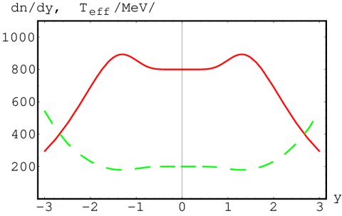
Figure 2: Same as Fig. 1 but utilizing a different form of the scaling function, ${\mathcal{V}}(s)=\sqrt{1+1.6s^{4}-2.6s^{8}}$, using a scale parameter $\dot{Z}_{0}^{2}=1$, $n_{0}t_{0}=800$ and $T_{0}(t_{0}/\tau_{f})^{1/\kappa}=200$ MeV, corresponding to a two-peaked rapidity distribution.

5 Cylindrically symmetric solutions

In this section, we describe a new family of exact analytic solutions of relativistic hydrodynamics, with cylindrically symmetric flow, overcoming the second of shortcoming of the well known boost-invariant Hwa-Bjorken solution [9, 10]. However, we do not address both shortcomings simultaneously yet. The physical motivation for this study is to consider the time evolution of central collisions in ultra-relativistic heavy-ion physics within the framework of an analytic approach. From now on, $x^{\mu}=(t,r_{x},r_{y},r_{z})\equiv(t,{\bf r})$ and $k^{\mu}=(E,k_{x},k_{y},k_{z})\equiv(E,{\bf k})$ with $E^{2}-{\bf k}^{2}=m^{2}$.

As we are primarily interested in the effects of finite transverse size and the development of transverse flow, we assume that the longitudinal flow component is boost-invariant,

$$v_{z}(t,r_{z})=\frac{r_{z}}{t}.$$ (40)

We search for self-similar solutions, that are scale dependent in the transverse directions, and depend only on the transverse radius variable $r_{t}=\sqrt{r_{x}^{2}+r_{y}^{2}}$ through the scaling variable

$$s=\frac{r_{x}^{2}+r_{y}^{2}}{R^{2}},$$ (41)

and the longitudinal proper time $\tau_{z}=\sqrt{t^{2}-r_{z}^{2}}$ and assume that, in the frame where $v_{z}=0$ (longitudinal proper frame), the transverse motion corresponds to a Hubble type of self-similar transverse expansion,

$$v_{x}^{*}(\tau_{z},r_{z}) = {\frac{\dot{R}(\tau_{z})}{R(\tau_{z})}}r_{x}\,,\qquad v_{y}^{*}(\tau_{z},r_{z})\,=\,{\frac{\dot{R}(\tau_{z})}{R(\tau_{z})}}r_{y}\,,$$ (42)

where $\dot{R}=dR(\tau_{z})/d\tau_{z}$ and hereafter we will designate by starred symbols the variables in the longitudinal proper frame. We assume that the scale $R$ depends on time only through the longitudinal proper time, $\tau_{z}$.

In a relativistic notation, the above form may be parametrized as

$$u^{\mu} = (\cosh\zeta\cosh\xi,\sinh\xi\frac{r_{x}}{r_{t}},\sinh\xi\frac{r_{y}}{r_{t}},\sinh\zeta\cosh\xi),$$ (43)

$$\tanh\xi = {\frac{\dot{R}(\tau_{z})}{R(\tau_{z})}}r_{t}=v_{t}^{*}=\gamma_{l}v_{t}\,,\qquad\mbox{\rm or}\quad\cosh\xi\,=\,\frac{1}{\sqrt{1-\dot{R}^{2}s}}\equiv\gamma_{t}^{*}\,,$$ (44)

$$\cosh\zeta = \frac{t}{\tau_{z}}\equiv\gamma_{l}\,.$$ (45)

The space-time rapidity $\eta$ is still defined by eq. (20). For a scaling longitudinal flow we obtain $\zeta=\eta\,$. Using the above ansatz for the flow velocity distribution, we find that the continuity equation is solved by the form

$$n(t,r_{x},r_{y},r_{z})=n_{0}\left(\frac{\tau_{z0}R_{0}^{2}}{\tau_{z}R^{2}}\right)\frac{1}{\cosh\xi}{\mathcal{G}}(s),$$ (46)

where ${\mathcal{G}}(s)$ is an arbitrary non-negative function of the scaling variable $s$ and $n_{0}\,$, $\tau_{z0}$ and $R_{0}$ are normalization constants. We use the convention $n_{0}=n(t_{0},0,0,0)$, $\tau_{z0}=\tau_{z}(t_{0},r_{z0})$ and $R_{0}=R(\tau_{z0})$, where $r_{z0}$ is such that, together with $t_{0}\,$, satisfies eq. (40). This implies that ${\mathcal{G}}(s=0)=1$. The temperature equation, eq. (9), is solved by

$$T(t,r_{x},r_{y},r_{z})=T_{0}\left(\frac{\tau_{z0}R_{0}^{2}}{\tau_{z}R^{2}}\frac{1}{\cosh\xi}\right)^{1/\kappa}{\mathcal{F}}(s).$$ (47)

The constants of normalization are $T_{0}=T(t_{0},0,0,0)$ and ${\mathcal{F}}(0)=1$. We find that the solution is independent of the form of the function ${\mathcal{F}}(s)$, provided that ${\mathcal{F}}(s)>0$.

Using a similar technique as in section 3, we obtain a transcendental equation for $\dot{R}^{2}$, and $s$. This equation has a particular solution if

$$\dot{R}=\dot{R}_{0}=\mbox{\rm Const}.$$ (48)

In this case, the acceleration of the radius parameter vanishes, $\ddot{R}=0$, and the solution is $R=R_{0}+\dot{R}_{0}(\tau_{z}-\tau_{z0})$. The relativistic Euler equation reduces to

$$\left(1+\frac{1}{\kappa}\right)\left(\frac{R\dot{R}}{\tau_{z}}+3\dot{R}^{2}\right)=2(1-s\dot{R}^{2})\left[\log{\mathcal{G}}(s){\mathcal{F}}(s)\right]^{\prime}\ ,$$ (49)

where the lhs depends only on $\tau_{z}$ while the rhs is only a function of the variable $s$, hence both sides are constant. This implies that $\frac{R}{\tau_{z}}=\dot{R}_{0}\,,$thus $R_{0}=\dot{R}_{0}\tau_{z0}\,$. Thus the origin of the time axis (fixed by the assumption of the scaling longitudinal flow profile) coincides with the vanishing value of the transverse radius parameters.

The solutions can be casted in a relatively simple form by introducing the proper time $\tau$,

$$\tau = \sqrt{\tau_{z}^{2}-r_{t}^{2}}\,=\,\sqrt{t^{2}-r_{x}^{2}-r_{y}^{2}-r_{z}^{2}}.$$ (50)

Using this natural variable we find that

$${\mathbf{v}} = \frac{{\mathbf{r}}}{t},\qquad\mbox{\rm or}\qquad u^{\mu}\,=\,\frac{x^{\mu}}{\tau}.$$ (51)

Thus the velocity field of our solution corresponds to the flow field of the spherically symmetric scaling solution and to the Hubble flow of the Universe. However, in the scaling solution the temperature and the pressure distributions are dependent only on the proper time $\tau$, while in our case both the density and the temperature distributions are generally dependent on the scale variable $s$ in the transverse direction.

As the solution is relativistic, and it is defined in the positive light-cone, given by $\tau\geq 0$, we obtain a constraint for the transverse coordinate, $r_{t}\leq\tau_{z}$. This together with the solution for the scale $R$, implies that the scaling variable has to satisfy the constraint $s\dot{R}_{0}^{2}\leq 1$, which corresponds to the limitation that the velocity of the fluid can not exceed the speed of light.

By substituting $R=\dot{R}_{0}\tau_{z}$ into the Euler equation, eq.(49), one obtains

$$\frac{d}{ds}\log\left[(1-s\dot{R}_{0}^{2})^{2(1+1/\kappa)}{\mathcal{G}}(s){\mathcal{F}}(s)\right]=0\,,$$ (52)

which gives, together with the condition ${\mathcal{G}}(0){\mathcal{F}}(0)=1$,

$${\mathcal{G}}(s){\mathcal{F}}(s)=(1-\dot{R}_{0}^{2}s)^{-2(1+1/\kappa)}.$$ (53)

In this family of solutions, the scaling functions for the temperature and the density distribution are thus not independent. However, a constraint is given for their product, hence one of them can be chosen as an arbitrary positive function. For clarity, let us introduce new forms of the scaling functions as

$${\mathcal{T}}(s) = {\mathcal{F}}(s)(1-\dot{R}_{0}^{2}s)^{2/\kappa},$$ (54)

$${\mathcal{V}}(s) = {\mathcal{G}}(s)(1-\dot{R}_{0}^{2}s)^{2}.$$ (55)

Then the constraint can be casted to the simple form of ${\mathcal{V}}(s){\mathcal{T}}(s)=1$. This construction for the scaling functions of the transverse density and temperature profiles coincides with the method, that we developed for the solution of the relativisitic hydrodynamical equations in the (1+1) dimensional problem, but here the transverse flow has a two-dimensional distribution, so the exponents and the scaling variables had to be re-defined accordingly.

Let us summarize our new family of solutions of the 1+3 dimensional relativistic hydrodynamics for cylindrically symmetric systems by substituting the results to the density, temperature and pressure profiles.

We obtain

$${\mathbf{v}} = \frac{\mathbf{r}}{t},\quad\mbox{\rm for}\quad|{\bf r}|\leq t,$$ (56)

$$s = \frac{r_{t}^{2}}{\dot{R}^{2}_{0}\tau_{z}^{2}},\quad\mbox{\rm for}\quad{r_{t}}\leq\tau_{z},$$ (57)

$$n(t,{\mathbf{r}}) = n_{0}\left(\frac{\tau_{z0}}{\tau}\right)^{3}{\mathcal{V}}(s),$$ (58)

$$p(t,{\mathbf{r}}) = p_{0}\left(\frac{\tau_{z0}}{\tau}\right)^{3+3/\kappa},$$ (59)

$$T(t,{\mathbf{r}}) = T_{0}\left(\frac{\tau_{z0}}{\tau}\right)^{3/\kappa}\frac{1}{{\mathcal{V}}(s)},$$ (60)

where $p_{0}=n_{0}T_{0}$. Note that the scaling variable $s$ is invariant for boosts in the longitudinal direction, and it is rotation-invariant in the transverse direction, but $s$ is not boost-invariant in the transverse directions. Hence we have generated cylindrically symmetric, longitudinally boost invariant solutions of relativistic hydrodynamics. In the longitudinal direction, these solutions are homogeneous, boost-invariant and also scale-invariant. Due to this reason, the observable rapidity distribution is

$$\frac{dN}{dy}=\mbox{\rm const},$$ (61)

a flat distribution, corresponding to the ultra-relativistic nature of the solution in the longitudinal direction (where $y=0.5\log[(E+k_{z})/(E-k_{z})]$ is the rapidity of a particle with four-momentum $(E,{\bf k})$ and $dn/dy$ is the rapidity distribution of particle density).

A new hydrodynamical solution is assigned to each non-negative function ${\mathcal{V}}(s)$, similarly to the cases of the non-relativistic solutions of ref. [18] and the 1+1 dimensional relativistic solution of the previous section. Note that the solutions are valid also for massive particles, the form of the solution is independent of the value of the mass $m$. The form of solutions depends parameterically on $\kappa$, that characterizes the equation of state.

We have obtained new solutions of the (1+3) dimensional relativistic hydrodynamical equations which describe a self-similar, streaming flow. In the case of $\dot{R}=1$ and ${\mathcal{V}}(s)=1$ we recover the spherically symmetric scale-invariant solution. This means that, in this limiting case, the pressure, the density and the temperature profiles depend only on the proper time $\tau$. In general case, however, our solution depends not only on the characteristic scale $R$ but also on the arbitrary scaling function ${\mathcal{V}}(s)$.

6 Summary

We have found a new family of both 1+1 dimensional, longitudinally expanding, and 1+3 dimensional, cylindrically symmetric, adiabatic solutions of relativistic hydrodynamics with conserved particle number. These families of solutions solves the continuity equation and the conservation of the energy - momentum tensor of a perfect fluid, assuming simple equations of state, given by Eqs.(4) and (5). The mass of the particles $m$ and $\kappa=\partial\epsilon/\partial p=1/c_{s}^{2}$ are free parameters of the solution. The well-known scale-invariant solution, has been obtained in the $m=0$ approximation. Interestingly, our generalizations resulted in additional freedom in the solution.

In the new 1+1 dimensional hydro solutions, the flow field coincides with that of the Hwa-Bjorken solution. In principle, the shape of the measurable rapidity distribution, $dN/dy$ plays the role of an arbitrary scaling function in our solution, and we obtain that the effective temperature of the transverse momentum distribution becomes rapidity dependent. Assuming that $dN/dy$ is a slowly varying function of the rapidity $y$, we find that the effective temperature is proportional to the inverse of the rapidity distribution, $T_{\mathrm{eff}}(y)\propto(dN/dy)^{-1}$.

In 1+3 dimensions, even the flow velocity field deviates from Hwa-Bjorken solution. We find that the only exact solution in the considered class corresponds to a scaling 3-dimensional flow, similar to the Hubble flow of the Universe. Although the pressure distribution is only proper-time dependent, this pressure is a product of the local number density and the local temperature, hence one of these can be chosen in an arbitrary manner.

The essential result of our paper is that we found a rich family of exact analytic solutions of relativistic hydrodynamics that contain both a longitudinal Hwa-Bjorken flow (that is frequently utilized in estimations of observables in high energy heavy ion collisions) and a relativistic transverse flow (whose existence is evident from the analysis of the single particle spectra at RHIC and SPS energies [23, 24, 25, 26]).

Acknowledgments: T. Cs. would like to thank L.P. Csernai, B. Lukács and J. Zimányi for inspiring discussions during the initial phase of this work, and to Y. Hama, G. Krein and S. S. Padula for their kind hospitality during his stay at USP and IFT, São Paulo, Brazil. This work has been supported by a NATO Science Fellowship (T. Cs.), by the OTKA grants T026435, T029158, T034269 and T038406 of Hungary, the NWO - OTKA grant N 25487 of The Netherlands and Hungary, and the grants FAPESP 00/04422-7, 99/09113-3, 02/11344-8, PRONEX 41.96.0886.00, FAPERJ E-26/150.942/99, and CNPq, Brazil.

References

- [1] L.P. Csernai, Introduction to Relativistic Heavy Ion Collisions, John Wiley and Sons, 1994.
- [2] D. Teaney, J. Lauret and E.V. Shuryak, nucl-th/0110037 v1.
- [3] T. Hirano, K. Morita, S. Muroya and C. Nonaka, nucl-th/0110009 v1.
- [4] P.F. Kolb, U. Heinz, P.Huovinen, K.J. Eskola and K. Tuminen, hep-ph/0103234 v3, Nucl. Phys. A696 (2001) 197-215.
- [5] C.E. Aguiar, T. Kodama, T. Osada, Y. Hama, J. Phys. G27 (2001) 75-94.
- [6] C.E. Aguiar, Y. Hama, T. Kodama, T. Osada, Nucl. Phys. A698 (2002) 639-642.
- [7] I.M. Khalatnikov, Zhur. Eksp. Teor. Fiz. 27 (1954) 529.
- [8] L.D. Landau, Izv. Akad. Nauk SSSR 17 (1953) 51; in “Collected papers of L.D. Landau” (ed. D. Ter-Haar, Pergamon, Oxford, 1965) p. 569-585.
-
[9]
R.C. Hwa, Phys. Rev. D10 (1974) 2260;
C.B. Chiu and K.-H. Wang, Phys. Rev. D12 (1975) 272;
C.B. Chiu, E.C.G. Sudarshan and K.-H. Wang, Phys. Rev. D12 (1975) 902;
M. I. Gorenstein, V. I. Zhdanov and Yu. M. Sinyukov, Sov. Phys. JETP 47 (78) 435.
K. Kajantie and L. D. McLerran, Phys. Lett. B 119 (1982) 203.
K. Kajantie and L. D. McLerran, Nucl. Phys. B 214 (1983) 261.
- [10] J.D. Bjorken, Phys. Rev. D27 (1983) 140.
- [11] T.S. Biró, Phys.Lett. B474 (2000) 21-26.
- [12] T.S. Biró, Phys.Lett. B487 (2000) 133-139.
- [13] J. Bondorf, S. Garpman and J. Zimányi, Nucl. Phys. A296 (1978) 320.
- [14] J.N. De, S.I.A. Garpman, D. Sperber, J.P. Bondorf and J. Zimányi, Nucl. Phys. A305 (1978) 226.
- [15] T. Csörgő, B. Lörstad and J. Zimányi; Phys. Lett. B338 (1994) 134; nucl-th/9408022.
- [16] J. Helgesson, T. Csörgő, M. Asakawa and B. Lörstad, Phys. Rev. C56 (1997) 2626.
- [17] P. Csizmadia, T. Csörgő and B. Lukács, nucl-th/9805006, Phys. Lett. B 443 (1998) 21.
- [18] T. Csörgő, nucl-th/9809011.
- [19] S.V. Akkelin, T. Csörgő, B. Lukács, Yu.M. Sinyukov and M. Weiner, Phys. Lett. B 505 (2001), 64.
- [20] T. Csörgő, S.V. Akkelin, Y. Hama, B. Lukács and Yu.M. Sinyukov, hep-ph/0108067, accepted for publication in Phys. Rev. C.
- [21] T. Csörgő, arXiv:hep-ph/0111139.
- [22] T. Csörgő and B. Lörstad, Phys. Rev. C54 (1996) 1390; T. Csörgő and B. Lörstad, Nucl. Phys. A590 (1995) 465c.
- [23] W. Broniowski and W. Florkowski, Phys. Rev. Lett. 87 (2001) 272302 [arXiv:nucl-th/0106050].
- [24] W. Florkowski and W. Broniowski, Acta Phys. Polon. B 33 (2002) 1629 [arXiv:nucl-th/0203058].
-
[25]
W. Florkowski and W. Broniowski,
arXiv:nucl-th/0212052;
W. Broniowski, A. Baran and W. Florkowski, arXiv:nucl-th/0212053. - [26] T. Csörgő and A. Ster, arXiv:nucl-th/0207016.