FLOW EQUATIONS FOR HAMILTONIANS FROM CONTINUOUS UNITARY TRANSFORMATIONS

By

Bruce Bartlett

Thesis presented in partial fulfilment of the requirements for the degree of

MASTER OF SCIENCE at the University of Stellenbosch.

Supervisors : Professor F.G. Scholtz

Professor H.B. Geyer

April 2003

DECLARATION
I, the undersigned, hereby declare that the work contained in this thesis is my own original work and that I have not previously in its entirety or in part submitted it at any university for a degree.

  Signature                                                             Date

ABSTRACT

This thesis presents an overview of the flow equations recently introduced by Wegner. The little known mathematical framework is established in the initial chapter and used as a background for the entire presentation. The application of flow equations to the Foldy-Wouthuysen transformation and to the elimination of the electron-phonon coupling in a solid is reviewed. Recent flow equations approaches to the Lipkin model are examined thoroughly, paying special attention to their utility near the phase change boundary. We present more robust schemes by requiring that expectation values be flow dependent; either through a variational or self-consistent calculation. The similarity renormalization group equations recently developed by Glazek and Wilson are also reviewed. Their relationship to Wegner’s flow equations is investigated through the aid of an instructive model.

OPSOMMING

Hierdie tesis bied ’n oorsig van die vloeivergelykings soos dit onlangs deur Wegner voorgestel is. Die betreklik onbekende wiskundige raamwerk word in die eerste hoofstuk geskets en deurgans as agtergrond gebruik. ’n Oorsig word gegee van die aanwending van die vloeivergelyking vir die Foldy-Wouthuysen transformasie en die eliminering van die elektron-fonon wisselwerking in ’n vastestof. Onlangse benaderings tot die Lipkin model, deur middel van vloeivergelykings, word ook deeglik ondersoek. Besondere aandag word gegee aan hul aanwending naby fasegrense. ’n Meer stewige skema word voorgestel deur te vereis dat verwagtingswaardes vloei-afhanklik is; óf deur gevarieerde óf self-konsistente berekenings. ’n Inleiding tot die gelyksoortigheids renormerings groep vergelykings, soos onlangs ontwikkel deur Glazek en Wilson, word ook aangebied. Hulle verwantskap met die Wegner vloeivergelykings word bespreek aan die hand van ’n instruktiewe voorbeeld.

ACKNOWLEDGEMENTS

The realization of this thesis would not have been possible without financial assistance from Stellenbosch University, the National Research Foundation (NRF) and the Harry Crossley Foundation. The financial assistance of the Department of Labour (DoL) towards this research is hereby acknowledged. Opinions expressed and conclusions derived at, are those of the author and are not necessarily to be attributed to the DoL.

Introduction

From the early days of Heisenberg’s matrix mechanics, it became clear that the language in which quantum physics described the world was in terms of matrices and linear operators. Specifically, the physical states of a system, and the values of any physical observable, were intimately connected with the mathematical problem of finding the eigenvectors and eigenvalues of a special Hermitian operator known as the Hamiltonian of the system. Simply put, the central problem of quantum mechanics is to diagonalize large (mostly infinite) matrices.

Of course, this grand problem is severely and thoroughly intractable, and sophisticated approximation schemes must be employed to obtain a grip on the nature of the solution. Moreover, the initial Hamiltonian is often expressed in terms of microscopic variables in such a way that it obscures the larger scale dynamics of the system. Before one attempts to solve for the energies and eigenstates of the system, we should first understand how the Hamiltonian works. In other words, one often requires an equivalent description of the same physical system, expressed in more familiar terms. This is expressed on the mathematical level by finding a unitarily equivalent Hamiltonian which can be viewed as a renormalization of the original theory, in the sense that the constants appearing in the model have been modified in order to accommodate the transformed nature of the Hamiltonian.

Such renormalization procedures have existed for a long time in the context of both quantum mechanics and statistical physics, and invariably result in a set of flow equations for the parameters present in the Hamiltonian [2]. In statistical physics one is normally interested in how the correlation between different microscopic elements of the system behaves as the length scale increases. Often this means “integrating out” the smaller length scales so as to provide an effective theory on the larger scale. In quantum field theory, one is interested in redefining coupling constants so as to reconcile them with their physically measurable counterparts.

Recently, Wegner [3] and independently, Glazek and Wilson [4, 5], have developed a new framework for flow equations. The authors have approached the subject from different contexts; the former from condensed matter physics and the latter from light-front quantum chromodynamics. Both approaches, though, are similar in style and purpose. Their distinction over previous methods is expressed in the title of the present thesis. Specifically, the flow equations are written directly in terms of the Hamiltonian, and do not involve the Lagrangian framework with their associated path integral methods. Secondly, the flow equations are continuous, as opposed to other methods which take place in discrete steps. Thirdly, the flow equations are unitary, so that no information about the system is lost. The transformed Hamiltonian is completely equivalent to the initial Hamiltonian at each point during the flow. Finally, the flow equations are designed to diagonalize or block-diagonalize the Hamiltonian (in Wegner’s scheme), or to continuously eliminate matrix elements involving large energy jumps, so as to render the Hamiltonian more and more band diagonal (in Glazek and Wilson’s scheme).

The purpose of this study is to present an overview of this new field, as well as to present new techniques which have proved useful. The little known general mathematical framework of flow equations is utilized extensively so as to provide a unified and unique presentation of the subject. A specific model from nuclear physics, the Lipkin model, is used as a central example against which to test various approaches.

The material is organized in the following way. In Chapter 1 Wegner’s flow equation is introduced and solved perturbatively. The mathematical framework behind the flow equation is presented and the steepest descent nature of the flow is revealed. The chapter concludes with considering two modifications of Wegner’s flow equation, namely Safonov’s one step scheme and block-diagonal flow equations. Chapter 2 discusses two pedagogical applications of flow equations to familiar problems. The Foldy-Wouthuysen transformation of the Dirac equation is derived using the new framework in a novel and illuminating way. Flow equations are also used as a means of renormalizing the electron-phonon interaction in solid-state physics into an effective electron-electron attraction term. This approach is compared with previous results using unitary transformations such as that of Fröhlich.

Chapter 3 introduces the Lipkin model and explains the phase transition present in the model. As a background to further discussion, numerical results are presented using brute force diagonalization of the matrix and numerical solution of the flow equations. This sets the stage for an overview of three separate flow equations treatments of the model, all of which fail to accommodate the second phase in a satisfying manner. Our own new method is presented which revolves around tracking the ground state during the flow, and proves to be of some use in treating both phases in a consistent way. Two approaches are presented, the first of which uses an external variational calculation while the other uses a self-consistent approximation. Other possible approaches are also considered, and the merits and drawbacks of each scheme are enumerated. The chapter ends with a discussion and summary of the important features of each approach.

Chapter 4 addresses the important question of how flow equations work relate to renormalization. It is here that Glazek and Wilson’s similarity renormalization group is presented, and compared to Wegner’s scheme. The renormalization properties of the flow equations are elucidated by considering two examples, one a toy model designed by Glazek and Wilson and the other the familiar electron-phonon problem.

The philosophy behind this work has been to attempt to expound all the finer details carefully, and some concepts are explained repeatedly. The author has tried to follow the sound advice given by Quintilian, 1900 years ago:

One should not aim at being possible to understand, but at being impossible to misunderstand.

Contents

1. Introduction
2. 1 Flow equations
   1. 1.1 Wegner’s flow equation
   2. 1.2 Perturbative solution
   3. 1.3 Mathematics of flow equations
      1. 1.3.1 Preliminaries
      2. 1.3.2 The manifold of unitarily equivalent matrices
      3. 1.3.3 The steepest descent formulation
   4. 1.4 Other methods
      1. 1.4.1 One step continuous unitary transformations
      2. 1.4.2 Block-diagonal flow equations
3. 2 Examples of flow equations
   1. 2.1 Foldy-Wouthuysen transformation
   2. 2.2 The electron-phonon interaction
      1. 2.2.1 Fröhlich’s Transformation
      2. 2.2.2 Flow equations approach
      3. 2.2.3 ${\cal L}$ Ordering and the generator expansion
      4. 2.2.4 Comparison with Fröhlich’s Results
4. 3 The Lipkin model
   1. 3.1 Introduction
      1. 3.1.1 The model
      2. 3.1.2 Phase transition
   2. 3.2 Some preliminary numerics
      1. 3.2.1 Brute force diagonalization
      2. 3.2.2 Exact numerical solution of flow equations
   3. 3.3 Pirner and Friman’s treatment
      1. 3.3.1 First scheme
      2. 3.3.2 Second scheme
      3. 3.3.3 Discussion
   4. 3.4 Mielke’s matrix element treatment
   5. 3.5 Stein’s bosonization method
   6. 3.6 Tracking the ground state
      1. 3.6.1 First scheme
      2. 3.6.2 Second scheme
   7. 3.7 Self-consistent linearization
   8. 3.8 Other flow equations approaches to the Lipkin model
      1. 3.8.1 Operator differential equations
      2. 3.8.2 Moment preservation
      3. 3.8.3 Generator flow
   9. 3.9 Discussion
5. 4 Flow equations and renormalization
   1. 4.1 Glazek and Wilson’s similarity renormalization
   2. 4.2 Wegner’s flow equation and the similarity renormalization group
   3. 4.3 Renormalization in action
      1. 4.3.1 Glazek and Wilson’s discrete 2-d delta function model
      2. 4.3.2 Renormalization of the electron-phonon interaction
6. 5 Conclusion
7. Bibliography

Chapter 1 Flow equations

1.1 Wegner’s flow equation

We intend to perform a continuous unitary transformation on an initial Hamiltonian $H_{0}$ in such a way that the Hamiltonian flows towards diagonal form. By a continuous unitary transformation we mean that the Hamiltonian travels on a unitary path

$$H(\ell)=U(\ell)H_{0}U^{\dagger}(\ell),\quad H(0)=H_{0}.$$ (1.1)

The flow of the Hamiltonian can be expressed in an infinitesimal form by computing the derivative with respect to $\ell$:

$$\frac{dH}{d\ell} = \frac{dU}{d\ell}H(0)U^{\dagger}+UH(0)\frac{dU^{\dagger}}{d\ell}$$ (1.2)

$$= \frac{dU}{d\ell}U^{\dagger}UH(0)U^{\dagger}-UH(0)U^{\dagger}\frac{dU}{d\ell}U^{\dagger}$$ (1.3)

$$= \frac{dU}{d\ell}U^{\dagger}H(\ell)-H(\ell)\frac{dU}{d\ell}U^{\dagger}$$ (1.4)

$$= [\eta(\ell),H(\ell)],$$ (1.5)

where the derivative of $UU^{\dagger}=1$ has been employed in the second line. Hence, the derivative of the Hamiltonian can be expressed as the commutator of an anti-Hermitian generator $\eta^{\dagger}=-\eta$ with the Hamiltonian,

$$\frac{dH}{d\ell}=[\eta(\ell),H(\ell)],$$ (1.6)

where $\eta(\ell)=\frac{dU}{d\ell}U^{\dagger}$. Instead of concentrating on the unitary transformation $U(\ell)$, one may instead shift interest onto the generator itself by recognizing equation (1.6) as the most general form of a unitary flow on the Hamiltonian. The idea is to choose $\eta$ so as to solve the problem, which in our case is diagonalizing $H_{0}$. The usual Jacobi iterative numerical method for diagonalizing a matrix performs a sequence of unitary transformations $U_{ij}$ on $H_{0}$:

$$H^{\prime}=U_{i_{N}j_{N}}\cdots U_{i_{1}j_{1}}H_{0}U^{\dagger}_{i_{1}j_{1}}\cdots U^{\dagger}_{i_{N}j_{N}}.$$ (1.7)

Each transformation $U_{ij}$ is designed to eliminate the off-diagonal term $H_{ij}$. In general the next unitary transformation will cause $H_{ij}$ to reappear, but due to the construction of the unitary transformations the new $H_{ij}$ has a reduced magnitude. In this way one obtains a sequence of Hamiltonians $H^{\prime(m)}$ which converge to diagonal form.

Wegner found a generator which will perform the diagonalization continuously:

$$\eta(\ell)=[\mbox{Diag}(H(\ell)),H(\ell)]\rightarrow\quad\eta_{ij}=H_{ij}(\varepsilon_{i}-\varepsilon_{j}).$$ (1.8)

Diag($H$) refers to the diagonal part of $H$. The $\varepsilon_{i}$ are simply the diagonal entries $H_{ii}$. To prove that this choice diagonalizes the Hamiltonian, we substitute the generator (1.8) into the general flow equation (1.6). With the convention that $v_{ij}$ is the $\ell$-dependent off-diagonal part of $H(\ell)$ (note that $v_{ii}=0$), we obtain the following differential equations for the diagonal and off-diagonal matrix elements,

$$\dot{\varepsilon_{i}} = 2\sum_{k}(\varepsilon_{i}-\varepsilon_{k})|v_{ik}|^{2}$$ (1.9)

$$\dot{v_{ij}} = -(\varepsilon_{i}-\varepsilon_{j})^{2}v_{ij}+\sum_{k}(\varepsilon_{i}+\varepsilon_{j}-2\varepsilon_{k})v_{ik}v_{kj},$$ (1.10)

where the dot indicates differentiation with respect to $\ell$. Eqs. (1.9) and (1.10) are Wegner’s flow equations written explicitly in matrix element form. The sum of the squares of the diagonal matrix elements must increase:

$$\frac{d}{d\ell}\sum_{i}\varepsilon_{i}^{2} = 2\sum_{i}\varepsilon_{i}\frac{d\varepsilon_{i}}{d\ell}$$ (1.11)

$$= 2\sum_{i,k}2\varepsilon_{i}(\varepsilon_{i}-\varepsilon_{k})|v_{ik}|^{2}$$

$$= 2\sum_{i,k}(\varepsilon_{i}-\varepsilon_{k})^{2}|v_{ik}|^{2}\geq 0.$$ (1.12)

Since the trace of a matrix remains invariant under unitary transformations,

$$\frac{d}{d\ell}\mbox{Tr}(H^{2}(\ell))=\frac{d}{d\ell}\left(\sum_{i}\varepsilon_{i}^{2}+\sum_{ij}|v_{ij}|^{2}\right)=0,$$ (1.13)

Eq. (1.12) implies that the off-diagonal elements must monotonically decrease until the only off-diagonal matrix elements that can possibly remain are those between states with equal diagonal matrix elements. We conclude that the choice of generator (1.8) has the remarkable property of causing the Hamiltonian to flow towards diagonality.

1.2 Perturbative solution

Let us now solve the flow equations (1.9) and (1.10), written in terms of the matrix elements, perturbatively. We assume that the initial Hamiltonian can be written as

$$H_{0}=D_{0}+gV_{0},$$ (1.14)

with $D_{0}$ and $V_{0}$ diagonal and off-diagonal respectively, and $g$ the bare coupling constant. We expand $\varepsilon_{i}(\ell)$ and $v_{ij}(\ell)$ in powers of $g$,

$$\varepsilon_{i}(\ell) = \varepsilon_{i}^{(0)}(\ell)+g\varepsilon_{i}^{(1)}(\ell)+g^{2}\varepsilon_{i}^{(2)}(\ell)+\cdots$$ (1.15)

$$v_{ij}(\ell) = gv_{ij}^{(1)}+g^{2}v_{ij}^{(2)}+\cdots$$ (1.16)

and substitute into the flow equations (1.9) and (1.10). The result up to second order in $g$ is

$$\varepsilon_{i}(\ell) = E_{i}+g^{2}\sum_{k}\frac{V_{ik}^{2}}{\Delta_{ik}}\left(1-e^{-2\Delta_{ik}^{2}\ell}\right)+\cdots$$ (1.17)

$$v_{ij}(\ell) = gV_{ij}e^{-\Delta_{ij}^{2}\ell}+g^{2}\sum_{k}\frac{V_{ik}V_{kj}(\Delta_{ik}+\Delta_{jk})}{\Delta^{2}_{ik}+\Delta^{2}_{kj}-\Delta^{2}_{ij}}\left(1-e^{-(\Delta^{2}_{ik}+\Delta^{2}_{kj}-\Delta^{2}_{ij})\ell}\right)e^{-\Delta^{2}_{ij}\ell}+\cdots$$ (1.18)

where $E_{i}=\langle i|D_{0}|i\rangle$, $V_{ij}=\langle i|V_{0}|j\rangle$ and $\Delta_{ij}=E_{i}-E_{j}$. Eqs. (1.17) and (1.18) should be seen as a generalization of ordinary Rayleigh-Schrödinger perturbation theory, which only concentrates on the series for the final diagonal form of the eigenvalues, $\varepsilon_{i}(\infty)$. The beauty of the flow equations result is that we now have an idea of precisely how the initial matrix $H_{0}$ is continuously diagonalized into its final form. To second order in $g$, the diagonal elements decay exponentially to the eigenvalues. The off-diagonal elements decay exponentially to zero in the first order, but follow a slightly more complicated route in second order.

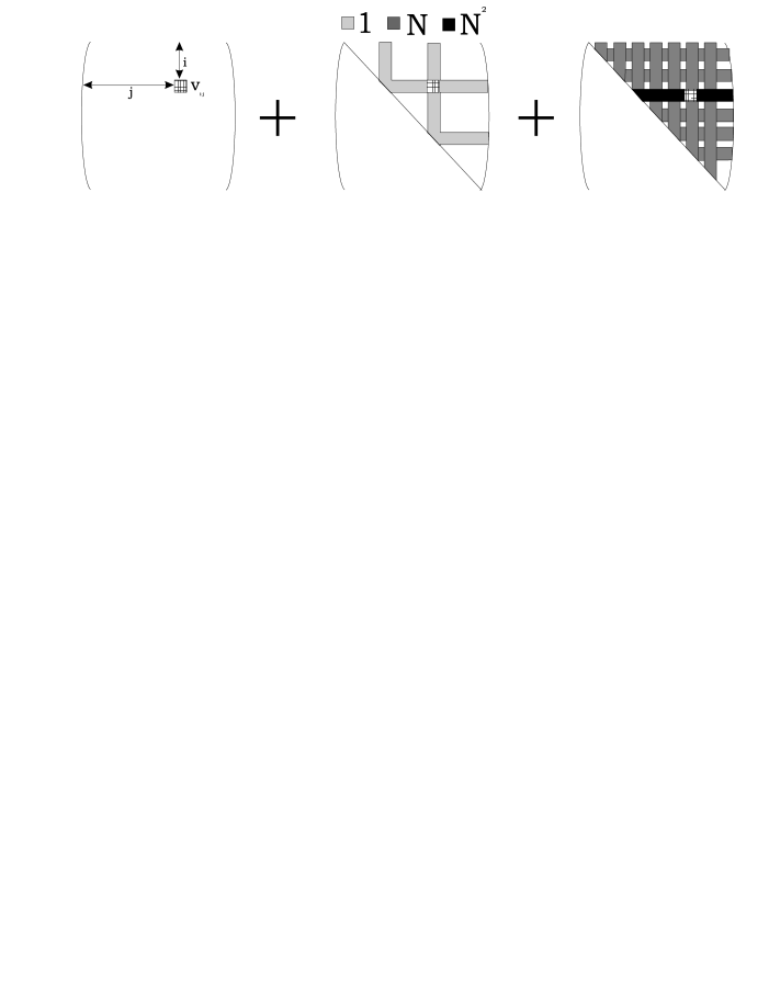
Figure 1.1: Coupling diagram illustrating how the off-diagonal element $v_{ij}$ depends on the other off-diagonal elements, order for order. Each colour is a different power of $N$, the dimension of the matrix. Since the Hamiltonian is hermitian, it is only necessary to display the upper-half of the matrix.

The perturbative solutions (1.17) and (1.18) also display in a concrete fashion the way in which the matrix elements are coupled and intermeshed to each other, by the constraint of remaining unitarily equivalent to the initial Hamiltonian. It is instructive to illustrate this by means of coupling diagrams, as in Fig. 1.1. The orders in perturbation theory for the off-diagonal elements are related schematically to the initial off-diagonal elements $V_{ij}$ by

$$v_{ij}(\ell)=gV_{ij}(\cdots)+g^{2}\sum_{k}{V_{ik}V_{kj}}(\cdots)+g^{3}\sum_{k,m}V_{ik}V_{im}V_{mk}(\cdots)+\cdots$$ (1.19)

Fig. 1.1 colours each matrix element according to the number of times it is counted in the above sum. The diagram offers a graphical illustration of the strength to which $v_{ij}$ is coupled to the other matrix elements, order for order.

1.3 Mathematics of flow equations

In this section the flow equations will be abstracted from their physical setting and discussed from a purely mathematical point of view.

Flow equations such as Wegner’s were, in fact, already discussed in the mathematical literature in 1983 [6], eleven years before Wegner’s paper. It is apparent from the physics literature that this fact is unknown. Although there are few mathematical papers that deal with the subject, there are some important aspects worth mentioning that classify precisely the status of a ‘flow equation’.

1.3.1 Preliminaries

Let us first review some basic notions of groups and manifolds. Let ${\cal G}$ be a group and ${\cal M}$ be a set. Then a map $\alpha:{\cal G}\times{\cal M}\rightarrow{\cal M}$ is an action of ${\cal G}$ on ${\cal M}$ if it satisfies the following conditions for all $g$, $h\in{\cal G}$ and $m\in{\cal M}$:

$$e\ast m=m\quad\mbox{and}\quad(gh)\ast m=g\ast(h\ast m),$$

where $e$ is the identity of the group $\cal G$. For $m\in{\cal M}$ let the orbit of $m$ be the action of the whole group ${\cal G}$ on $m$;

$$\mbox{Orbit}(m)={\cal G}\ast m=\{g\ast m:g\in{\cal G}\}.$$

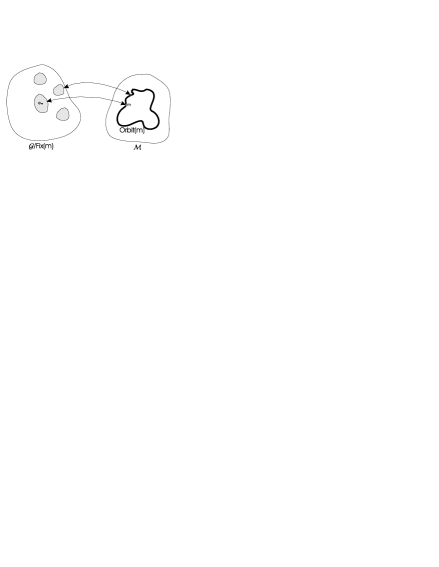
Figure 1.2: Orbit($m$) may be placed in one to one correspondence with ${\cal G}/\mbox{Fix}(m)$

Consider the set of elements of ${\cal G}$ that leave $m\in{\cal M}$ invariant:

$$\mbox{Fix}(m)=\{g\in{\cal G}:g\ast m=m\}.$$

It is easy to show that Fix($m$) is actually a normal subgroup of ${\cal G}$, so we may construct the quotient group ${\cal G}/$ Fix($m$). Now, every element in a given coset $g$Fix($m$) maps $m$ onto the same point in Orbit($m$). This gives us the following important 1-1 mapping between the elements of ${\cal G}/$ Fix($m$) and the orbit of $m$:

$${\cal G}/\mbox{Fix}(m)\rightarrow\mbox{Orbit}(m)\,:\,g\mbox{Fix}(m)\rightarrow g\ast m.$$

We are now in a position to state a well-known and important result [7].
Let ${\cal M}$ be a smooth manifold, and let ${\cal G}$ be a Lie group acting smoothly on ${\cal M}$, and let $m\in{\cal M}$. Then the orbit ${\cal G}\ast m$ of $m$ is a smooth homogeneous manifold of ${\cal M}$ with the following dimension:

$$\mbox{dim}({\cal G}\ast m)\,=\,\mbox{dim}({\cal G})-\mbox{dim Fix}(m).$$ (1.20)

1.3.2 The manifold of unitarily equivalent matrices

Let $H_{0}$ be a $n\times n$ Hermitian matrix and consider the class ${\cal C}$ of all matrices unitarily equivalent to it:

$${\cal C}(H_{0})=\{H\;:\;H\mbox{ is unitarily equivalent to }H_{0}\}.$$

Since two Hermitian matrices are unitarily equivalent if and only if there is a unitary transformation that connects the two, ${\cal C}$ is clearly equivalent to the action of the group of unitary matrices $U(n)$ on $\Lambda$, where $\Lambda$ is a diagonalized form of $H_{0}$ (there are $n!$ such forms if $H_{0}$ is nondegenerate since the eigenvalues may be shuffled down the diagonal) and the action is defined by $Q\ast\Lambda\equiv Q\Lambda Q^{\dagger}$. From the theorem (1.20) we now conclude that ${\cal C}(H_{0})$ is a smooth manifold. Let us now compute Fix($\Lambda$); that is, which unitary matrices $Q$ leave $Q\Lambda Q^{\dagger}=\Lambda$? Consider the case where the eigenvalues $\lambda_{i}$ of $\Lambda$ are all distinct. This is easy, since $Q\Lambda Q^{\dagger}=\Lambda$ $\Rightarrow$ $[Q,\Lambda]=0$ which means $Q$ must be diagonal. However, $QQ^{\dagger}=1$ thus

$$\mbox{Fix}(\Lambda)\,=\,\{\mbox{diag}(\alpha_{1},\alpha_{2},...,\alpha_{n})\,:\,|\alpha_{i}|=1\},$$

which is $n$-dimensional. If the eigenvalues are not distinct, say $\lambda_{i}=\lambda_{j}$, then care should be exercised since Q may have off diagonal entries at $q_{ij}$ and $q_{ji}$.

Since dim $U(n)=n^{2}$ we conclude that, providing the eigenvalues of $H_{0}$ are distinct, ${\cal C}(H_{0})$ is a smooth, compact, homogeneous manifold of dimension $n^{2}-n$. $\Box$

Indeed, this result could easily be anticipated since two $n\times n$ matrices $A$ and $B$ are unitarily equivalent if and only if their moments up to order $n$ are equal [44]:

$$\mbox{tr}(A^{i})\,=\,\mbox{tr}(B^{i}),\quad i=1..n$$ (1.21)

Since a complex Hermitian matrix has $n^{2}$ real degrees of freedom, these $n$ constraints gives the dimension of the set of matrices unitarily equivalent to $A$ as $n^{2}-n$. Unfortunately the equations in (1.21) do not help us to eliminate the redundant variables directly since the expressions in the traces are high order (up to $n$) polynomials in the matrix elements.

For those aficionados who think that all this effort to prove that the class of unitarily equivalent matrices is a smooth manifold is unnecessary, since just about all sets are manifolds anyway, consider the following counterexample. The set of unitarily equivalent $3\times 3$ tridiagonal matrices, in which two eigenvalues coincide, fails to be a manifold since it is homeomorphic to a figure eight [8].

Now that we have established that ${\cal C}(H_{0})$ is a manifold, we may go on to compute its Euler characteristic, its differential geometry and so on. We shall not follow this route, but simply mention two important examples:

• For $3\times 3$ real matrices the manifold is a sphere with 2 handles [9]. This is in contrast to the manifold of SO(3), a sphere with opposite points on the surface identified (Fig. 1.3(a)).

• For $3\times 3$ real tridiagonal matrices

  $$\left(\begin{array}[]{ccc}a_{1}&b_{1}&0\\ b_{1}&a_{2}&b_{2}\\ 0&b_{2}&a_{3}\end{array}\right),$$ (1.22)

  with distinct eigenvalues $\lambda_{1}>\lambda_{2}>\lambda_{3}$ the manifold breaks into four closed components $++$, $+-$, $-+$, $--$, depending on the signs of $b_{1}$ and $b_{2}$ ($+$$-$, for example, means $b_{1}\geq 0$, $b_{2}\leq 0$). The set $++$ is homeomorphic to a hexagon [8] (Fig. 1.3(b)).

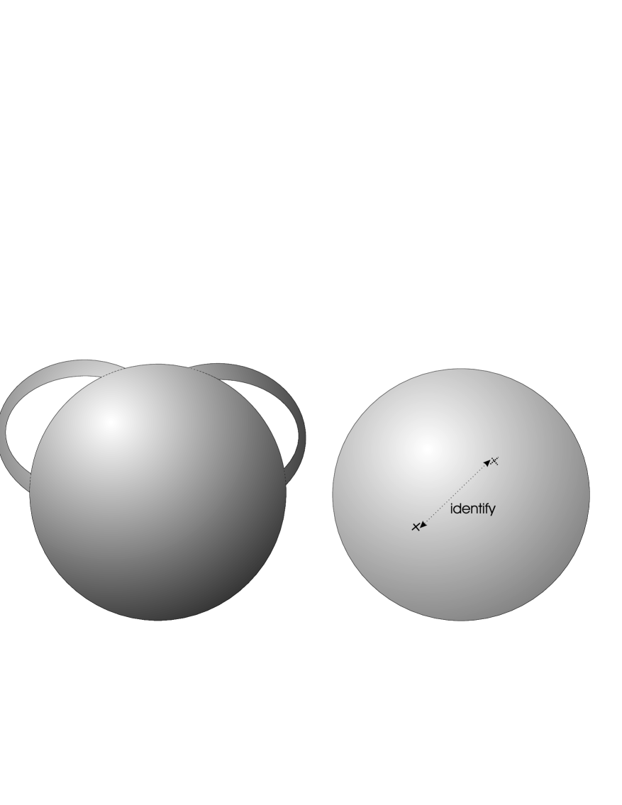
(a)

(b)

Figure 1.3: (a) The difference between the manifold of $3\times 3$ unitarily equivalent real matrices, and the manifold SO(3). (b) The $++$ section of $3\times 3$ real tridiagonal unitarily equivalent matrices is homeomorphic to a hexagon.

1.3.3 The steepest descent formulation

Here we follow the work of Refs. [10] and [11]. The flow equations can be placed into a more general framework based on the following problem:

Find $X\in{\cal C}(H_{0})$ that minimizes the function

$$F(X)=\|X-P(X)\|^{2}.$$ (1.23)

Here $\|\cdot\|$ means the Frobenius norm defined as

$$||X||=\sqrt{\left<X,X\right>},$$ (1.24)

where the standard trace inner product is intended, $\left<A,B\right>=\mbox{tr}(A^{\dagger}B)$. $P(X)$ is a projection of $X$ onto a subspace $\Phi$ of the space of $n\times n$ Hermitian matrices. In other words, we are trying to find the closest possible matrix to $\Phi$ under the constraint that it be unitarily equivalent to $H_{0}$. By choosing $\Phi$ appropriately the problem may be adapted to mathematical problems such as the inverse eigenvalue problem [12], Toda flows [13, 14] and displacement flows [14]. Physicists have yet to discover this formulation but it does define a precise framework for some problems, such as finding the Hamiltonian closest to block diagonal form, in a renormalization type scheme. The idea is simply to set up the steepest descent differential equations so as to maximally decrease $F(X)$ in each step. The flow may be viewed as taking place in the Hamiltonian space ${\cal C}(H_{0})$ and in the unitary matrix space SU($n$) simultaneously.

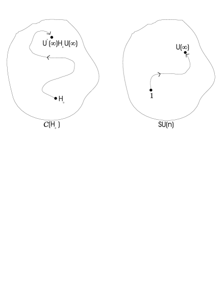
Figure 1.4: The flow may be viewed either on the level of the matrix elements themselves, or as a flow in the unitary matrices that accomplish the diagonalization.

In ${\cal C}(H_{0})$, the matrix begins at $H_{0}$ and ends when it is closest to $\Phi$. In SU($n$), the flow begins at the identity matrix and ends at the unitary matrix that accomplishes the job. We may restrict our attention to SU($n$) as opposed to U($n$) since any element of U($n$) can be written as $U=e^{i\phi}V$, with $V\in\mbox{U}(n)$, and the phase $\phi$ does not affect the transformed Hamiltonian.

It can easily be shown [10] that the only fixed point $X$ of the steepest descent of the objective function (1.23) in ${\cal C}(H_{0})$ occurs when $X$ commutes with its own projection:

$$\left[X,P(X)\right]=0$$

Thus to solve the eigenvalue problem, we may choose the subspace $\Phi$ to be either:
(1) the space of all diagonal matrices : $P(X)$ = Diag($X$), or
(2) a fixed diagonal matrix $N$ : $P(X)$ = $N$,
where $N$ is some arbitrary diagonal matrix with distinct entries chosen to ‘guide’ the equations. These choices work since

$$[X,D]_{ij}=0\;\Leftrightarrow\;X_{ij}(D_{jj}-D_{ii})=0,$$ (1.25)

where $D$ is a diagonal matrix. For (2) this implies that $X$ must be diagonal while in (1) $X_{ij}$ may still be non-zero for $i\neq j$, providing that the diagonal entries $X_{ii}$ and $X_{jj}$ are equal.

For completeness, we shall now illustrate the steps leading to the steepest descent flow equations for case (2). Let us then consider the objective function $\bar{F}$ in SU($n$),

$$\bar{F}(Q) = \|Q^{\dagger}H_{0}Q-N\|^{2}$$ (1.26)

$$= \mbox{tr}\left((Q^{\dagger}H_{0}Q-N)(Q^{\dagger}H_{0}Q-N)\right)$$ (1.27)

$$= \mbox{tr}(H_{0}^{2})+\mbox{tr}(N^{2})-2\mbox{tr}(Q^{\dagger}H_{0}QN).$$ (1.28)

Ignoring the terms which are independent of $Q$, the function we wish to maximize is tr($Q^{\dagger}H_{0}QN)$. The unitary matrix $Q$ will trace out a path $Q(\l)$. Consider a point $Q_{0}$ along this path. We parametrize its neighbourhood as

$$Q(\Omega)=Q_{0}\left(1+\Omega+\frac{\Omega^{2}}{2!}+\cdots\,\right)$$ (1.29)

with $\Omega$ anti-hermitian. To first order in $\Omega$ we have

$$\mbox{tr}\left((1-\Omega)Q_{0}^{\dagger}H_{0}Q_{0}(1+\Omega)N\right) = \mbox{tr}\left(Q_{0}^{\dagger}H_{0}Q_{0}\right)-\mbox{tr}\left(\Omega Q_{0}^{\dagger}H_{0}Q_{0}N\right)+$$ (1.31)

$$\qquad\qquad\qquad\mbox{tr}\left(Q_{0}^{\dagger}H_{0}Q_{0}\Omega.N\right)$$

Using the cyclic properties of the trace function gives

$$\mbox{tr}\left((1-\Omega)Q_{0}^{\dagger}H_{0}Q_{0}(1+\Omega)N\right)-\mbox{tr}\left(Q_{0}^{\dagger}H_{0}Q_{0}\right) = -\mbox{tr}(Q_{0}^{\dagger}H_{0}Q_{0}N\Omega)+\mbox{tr}(NQ_{0}^{\dagger}H_{0}Q_{0}\Omega)$$ (1.32)

$$= \mbox{tr}\left([N,Q_{0}^{\dagger}H_{0}Q_{0}]\Omega\right)$$ (1.33)

$$= \mbox{tr}\left([Q_{0}^{\dagger}H_{0}Q_{0},N]^{\dagger}\Omega\right)$$ (1.34)

$$= \left<[Q_{0}^{\dagger}H_{0}Q_{0},N],\,\Omega\right>.$$ (1.35)

Since we have worked to first order in $\Omega$ we see that $\left<[Q^{\dagger}H_{0}Q,N],\,\cdot\,\right>$ represents the gradient function at $Q$, in the sense that it accounts for the infinitesimal behavior of $\bar{F}$ there. Following the parameterization of the neighborhood (1.29), we choose $\dot{Q}=Q\Omega$, so now we can express the gradient flow as

$$Q^{\dagger}\dot{Q}=[Q^{\dagger}H_{0}Q,N],$$

or

$$\dot{Q}=Q[Q^{\dagger}H_{0}Q,N].$$ (1.36)

This equation evolves in SU($n$) and is cubic in $Q$. Let us now evaluate the projection of the flow equation in the space of hermitian matrices. Let $H=Q^{\dagger}H_{0}Q$. Then

$$\dot{H} = [N,Q^{\dagger}H_{0}Q]Q^{\dagger}H_{0}Q+Q^{\dagger}H_{0}Q[Q^{\dagger}H_{0}Q,N]$$ (1.37)

$$= -HNH+H^{2}N-HNH+NH^{2}$$ (1.38)

$$= \left[\,[N,H]\,,\,H\,\right],$$ (1.39)

which is the form of the flow equation we shall use for most of this work. Wegner’s original flow equation is recovered by choosing $\mbox{P}(X)=\mbox{Diag}(X)$ as in case(1) above. The analysis runs similarly to the one we have just presented. The flow equation in SU($n$) is

$$\dot{Q}=Q[Q^{\dagger}H_{0}Q,\mbox{Diag}(Q^{\dagger}H_{0}Q)],$$

while the corresponding flow in the Hermitian matrices is

$$\dot{H}=\left[[\mbox{Diag}(H),H],H\right],$$

which is precisely Wegner’s flow equation! To summarize, we see that Wegner’s flow equations determine steepest descent curves to diagonality in matrix space. The difference between the two cases presented above is that using $[N,H]$ as the generator produces steepest flow towards $N$, while $[\mbox{Diag}(H),H]$ produces steepest descent flow to the diagonalized form of $H_{0}$. Both generators cause $H$ to flow to diagonal form, with the latter achieving this slightly quicker. The advantage of the first formulation (using $N$) is that

• The equations are quadratic in $H$ and cubic in $Q$, while in the latter case they are cubic in $H$ and pentic in $Q$.

• By choosing an appropriate $N$ it may be possible to restrict the flow to some submanifold of ${\cal C}(H_{0})$, for instance the tridiagonal matrices. This is what we shall do in Chapter 3, in the context of the Lipkin model (see Eq. (3.14)).

• Whereas the only stable fixed point of the flow equations using $[N,H$] as generator is the final diagonal matrix, it is possible for the flow equations using $[\mbox{Diag}(H),H]$ to end with remaining offdiagonal elements between states with equal diagonal elements (see Secion 1.1). This is because these points are local minima in the objective function $F$, from which a steepest descent formulation will not escape.

• It can be shown [11] that the final diagonal matrix to which the flow proceeds has its eigenvalues listed down the diagonal in the same order as in $N$.

The last property follows from the fact that, if $H$ is diagonal,

$$F(H)\,=\,\|H-N\|^{2}=\sum_{i}(h_{ii}-n_{ii})^{2},$$

so that $F$ is minimized when $H$ is similarly ordered to $N$. This viewpoint clears up some of the confusion evident in the physics literature about these topics. Some authors have expressed reservations about using generators like $[N,H]$ instead of Wegner’s original choice [38]. Others, in order to gain the advantages mentioned above, have set up new generators [41]. In the mathematical framework we have presented here it has been shown that the flow equations are robust - quite generally, the differential equation to minimize the distance of $H$ to some subspace $P(H)$ is

$$\dot{H}=[[P(H),H],H].$$

1.4 Other methods

1.4.1 One step continuous unitary transformations

A simpler but less general diagonalization scheme is Safonov’s ‘one step’ unitary transformation [15, 16, 17, 18, 19]. The idea is to choose a fixed scalable generator instead of a completely dynamic generator as used in the steepest descent flow equations. We parametrize the transformations on the Hamiltonian as

$$H(\ell)=e^{\ell R}H_{0}e^{-\ell R},$$

where $R$ is a fixed anti-hermitian generator, and $\ell$ a parameter. This expression for $H(\ell)$ is a solution of the differential equation

$$\frac{dH}{d\ell}=[R,H(\ell)].$$ (1.40)

This should be compared to the more general steepest descent formulation

$$\frac{dH}{dl}=[\eta(l),H(l)]\qquad\eta(l)=[\mbox{Diag}(H(l)),H(l)].$$ (1.41)

It is clear that the steepest descent equation rotates $H$ around $\eta$ at each step, where $\eta$ evolves dynamically with $H$. Safonov’s method restricts $H$ to be rotated around a fixed $R$ at each step.

The method involves:

• parametrising the flow of $H$ in terms of operator combinations involving unknown $\ell$ dependent coefficients,

  $$H(\ell)=a_{1}(\ell)H_{1}+a_{2}(\ell)H_{2}+\cdots a_{N}(\ell)H_{N},$$ (1.42)

• Expanding the generator $R$ in terms of unknown ($\ell$ independent) anti-Hermitian terms,

  $$R=b_{1}R_{1}+b_{2}R_{2}+\cdots b_{M}R_{M}.$$ (1.43)

The two expansions (1.42) and (1.43) are then substituted into the flow equation (1.40), which results in a set of linear differential equations for the $a_{i}$. Solving these equations with the initial conditions provided by the parameter values in the initial Hamiltonian, we obtain the transformed Hamiltonian $H(\ell)$. In order to eliminate ‘inconvenient’ terms (i.e. the off-diagonal terms in a diagonalization scheme) one needs to set their coefficients (for example, for $\ell=1$) equal to zero; $a_{p}(1)=0$, for the unwanted $a_{p}$. This gives a second set of equations which determines the $b_{i}$ and hence $R$.

The advantage of Safonov’s one step scheme is that the differential equations to be solved are linear, since the generator is $\ell$-independent. The difficulty is that extra interaction terms are still generated, for almost any (useful) choice of $R$. Providing the transformation involved is reasonably small, these extra terms may be neglected. Another difficulty is that the static nature of the generator $R$ does not allow for the unitary transformation to change dynamically during the flow. This is evident when Safonov’s method is used to eliminate the electron-phonon interaction terms in an interacting electron system, as will be done in Section 2.2. It gives the same result as Fröhlich’s original expansion of the unitary transformation by the BCH formula, which is to be expected since the two approaches have much in common.

1.4.2 Block-diagonal flow equations

Perhaps it is asking too much to attempt to diagonalize the Hamiltonian of the relevant problem completely. One may impose a less grand requirement, by asking only that the Hamiltonian flows to block-diagonal form. The individual blocks may then be analysed separately. This manner of thinking lends itself to Hamiltonians in relativistic field theory, which do not conserve the number of particles. In this case one may attempt to find an effective Hamiltonian which decouples the Fock spaces with different number of particles from each other.

Wegner’s flow equation can be extended in a straightforward fashion for this purpose. The method is most clearly explained in Ref. [20], where it was applied to determine an effective $q\bar{q}$-interaction in QCD. A good overall reference can be found in Ref. [21], where it was applied to QED on the light front.

One divides the Hilbert space into two pieces, the $P$ and the $Q$ space. We have only used two spaces here for clarity but of course in a field theory one would divide it into an infinite number of $P_{i}$ Fock spaces, where $i$ labels the number of particles in the space. With a slight abuse of notation, let $P$ and $Q=1-P$ represent the projection operators onto the $P$ and $Q$ spaces respectively. We intend to transform the Hamiltonian using flow equations into block-diagonal form:

$$\left(\begin{array}[]{cc}PHP&PHQ\\ QHP&QHQ\end{array}\right)\rightarrow H(\infty)=\left(\begin{array}[]{cc}PH(\infty)P&0\\ 0&QH(\infty)Q\end{array}\right).$$ (1.44)

If we consider the $PHP$ and $QHQ$ blocks to be the “diagonal” part of the Hamiltonian $H_{d}$, and the $PHQ$ and $QHP$ blocks to be the “rest” $H_{r}$, then the usual Wegner formula would dictate that

$$\eta(\ell)=[H_{d}(\ell),H_{r}(\ell)]$$ (1.45)

is the choice of generator to employ. Indeed, this choice shall be proved shortly to propagate the Hamiltonian to block-diagonal form. Firstly note that the generator is always off-diagonal (in our block-diagonal sense of the term):

$$P\eta(\ell)P=Q\eta(\ell)Q=0.$$ (1.46)

Evaluating (1.45) in the two upper blocks gives

$$\frac{d}{d\ell}(PHP) = P\eta QHP-PHQ\eta P$$ (1.47)

$$\frac{d}{d\ell}(PHQ) = P\eta QHQ-PHP\eta Q.$$ (1.48)

To show that the Hamiltonian flows to block-diagonal form, we use a simple extension of the original Wegner matrix element proof from Section 1.1 by defining a measure of off-diagonality ${\cal O}=||PHQ||^{2}=\mbox{Tr}(PHQHP)$. Using the expressions for the flow in each block (1.47) and (1.48) we find its derivative to be

$$\frac{d{\cal O}}{d\ell} = \mbox{Tr}\left(P\eta Q(QHQHP-QHPHP)\right)+\mbox{Tr}\left((PHPHQ-PHQHQ)Q\eta P\right)$$ (1.49)

$$= 2\mbox{Tr}(P\eta Q\eta P)=-2\mbox{Tr}((Q\eta P)^{\dagger}Q\eta P)=-2||Q\eta P||^{2}\leq 0,$$ (1.50)

which proves that $H_{r}$ must decrease during the flow, leading to a block-diagonal Hamiltonian. This illustrates yet again how flexible double commutator flow equations such as Wegner’s can be.

It is important to compare the flow equations approach to constructing a block-diagonal effective Hamiltonian, and other previous approaches such as that of Lee and Suzuki [42]. This latter approach writes the transformed Hamiltonian as

$$H^{\prime}=e^{-\omega}He^{\omega}$$ (1.51)

and then requires that $H^{\prime}$ be block diagonal,

$$QH^{\prime}P=0$$ (1.52)

and that the generator only has nonzero entries in the bottom-left block,

$$\omega=Q\omega P$$ (1.53)

This latter requirement is inconsistent with the primed Hamiltonian $H^{\prime}$ remaining unitarily equivalent to $H$, since the generator $\omega$ is no longer anti-hermitian. The transformation though is still a similarity transformation, so that the eigenvalues of $H$ and $H^{\prime}$ coincide. The requirements (1.52) and (1.53) lead to a non-linear equation for the generator $\omega$, which must be solved perturbatively. The difference between this and the flow equations approach is that the latter remains a strictly unitary transformation. Furthermore, the differential flow equations constitute an approach whereby the Hamiltonian is transformed continuously. In contrast, the method of Lee and Suzuki attempts to find a one step transformation, although this is normally computed in a discrete iterative procedure.

Chapter 2 Examples of flow equations

For the benefit of the reader who is anxious to discover if flow equations have any merit with physical problems, we briefly review here two recent treatments. They have been chosen out of the myriad of other possibilities for pedagogical reasons, since the first is rather simple and rapidly leads to an exact but perturbative solution. The second is a good example of how flow equations can be applied in a condensed matter context, in order to find effective Hamiltonians. It illustrates the concepts of renormalization (this will be returned to in Section 4.3.2), and the ${\cal L}$ ordering operation, as well as dealing with unwanted newly-generated terms.

2.1 Foldy-Wouthuysen transformation

The Foldy-Wouthuysen transformation is a unitary transformation that decouples the upper and lower pairs of components in the Dirac equation. It is normally derived as an expansion in powers of $1/m$ [22]. We will derive it here using flow equations following Ref. [23], since it is a good example of a non-trivial problem that can be solved in a perturbative but exact treatment.

The initial Hamiltonian is (see eg. Ref. [22])

$$H_{0}=\vec{\alpha}\cdot\left(\vec{p}-\vec{A}(\vec{x})\right)+\beta m+eA_{0}(\vec{x}).$$

This Hamiltonian contains the $\vec{\alpha}$ terms which connect the upper and lower components of the Dirac spinor. The objective is to transform it to block-diagonal form. The key observation is that the matrix $\beta$ has the special property that

• The most general form of the Hamiltonian during the flow can be written as a sum of even and odd terms, which commute and anticommute respectively with $\beta$ (This statement will be justified shortly).

  $$H(\ell) = \cal{E}(\ell)+\cal{O}(\ell)$$ (2.1)

  $$\left[\cal{E}(\ell),\beta\right] = 0$$ (2.2)

  $$\{\cal{O}(\ell),\beta\} = 0.$$ (2.3)

• The required final Hamiltonian should commute with $\beta$ in order to be block-diagonal

  $$[H(\infty),\beta]=0.$$

To ensure steepest descent to block-diagonality we choose the generator as

$$\eta(\ell)=[\beta m,H(\ell)],$$ (2.4)

where the mass $m$ appears in order to formulate a perturbative solution in $1/m$. In this way we see that $\beta$ enters into both the generator (2.4) and into the form of the Hamiltonian during the flow, via the parity relations (2.2) and (2.3). Substituting the Hamiltonian (2.1) into the generator (2.4) gives

$$\eta(\ell)=2m\beta{\cal O}(\ell).$$

The initial even and odd components are

$${\cal E}(0) = \beta m+eA_{0}$$ (2.5)

$${\cal O}(0) = \vec{\alpha}\cdot(\vec{p}-e\vec{A}).$$ (2.6)

By applying the commutation relations (2.2) and (2.3) one sees that the flow equations can be written in the following closed form

$$\frac{d{\cal E}(\ell)}{d\ell} = 4m\beta{\cal O}^{2}(\ell)$$ (2.7)

$$\frac{d{\cal O}(\ell)}{d\ell} = 2m\beta[{\cal O}(\ell),{\cal E}(\ell)]$$ (2.8)

A word about such a closed form of equations is in order. ${\cal E}(\ell)$ and ${\cal O}(\ell)$ are not simply scalar coefficients but operator-valued functions of $\ell$. Nevertheless the usual rules of calculus can be used to treat (2.7) as if it was a system of differential equations in scalar variables. We now proceed to solve these equations perturbatively in $1/m$. In order to conveniently distinguish different orders we introduce the dimensionless flow parameter $s=m^{2}\ell$. Now we express ${\cal E}(s)$ and ${\cal O}(s)$ in orders of $1/m$. Since ${\cal E}(0)=\beta m+eA_{0}$ the expansion of ${\cal E}(s)/m$ contains terms starting with the zeroth order term

$$\frac{1}{m}{\cal E}(s)={\cal E}_{0}(s)+\frac{1}{m}{\cal E}_{1}(s)+\frac{1}{m^{2}}{\cal E}_{2}(s)+\cdots$$ (2.9)

while the expansion of ${\cal O}(s)$ starts with the first order

$$\frac{1}{m}{\cal O}(s)=\frac{1}{m}{\cal O}_{1}(s)+\frac{1}{m^{2}}{\cal O}_{2}(s)+\cdots$$ (2.10)

Substituting the expansions (2.9) and (2.10) into the flow equations (2.7), equating terms of the same order, and using the commutation relations (2.2) and (2.3) gives

$$\frac{d{\cal E}_{n}(s)}{ds} = 4\beta\sum_{k=1}^{n-1}{\cal O}_{k}(s){\cal O}_{n-k}(s)$$ (2.11)

$$\frac{d{\cal O}_{n}(s)}{ds} = -4{\cal O}_{n}(s)+2\beta\sum_{k=1}^{n-1}[{\cal O}_{k}(s),{\cal E}_{n-k}(s)].$$ (2.12)

These equations can be integrated to give the recursive type solution

$${\cal E}_{n}(s) = {\cal E}_{n}(0)+4\beta\int_{0}^{s}ds^{\prime}\sum_{k=1}^{n-1}{\cal O}_{k}(s^{\prime}){\cal O}_{n-k}(s^{\prime})$$ (2.13)

$${\cal O}_{n}(s) = {\cal O}_{n}(0)e^{-4s}+2\beta e^{-4s}\int_{0}^{s}ds^{\prime}e^{4s^{\prime}}\sum_{k=1}^{n-1}[{\cal O}_{k}(s^{\prime}),{\cal E}_{n-k}(s^{\prime})],$$ (2.14)

where the initial conditions are

$${\cal E}_{0}(0)=\beta,\;{\cal E}_{1}(0)=eA_{0}(\vec{x}),\;{\cal E}_{n}(0)=0\mbox{ if }n\geq 2$$ (2.15)

$${\cal O}_{1}(0)=\vec{\alpha}\cdot\left(\vec{p}-\vec{A}(\vec{x})\right),\;{\cal O}_{n}(0)=0\mbox{ if }n\geq 2.$$ (2.16)

As expected, we see that ${\cal O}_{n}(s)$ goes exponentially to zero as $s\rightarrow\infty$, so that the final Hamiltonian is indeed block diagonal. We may now proceed to evaluate ${\cal E}_{n}(\infty)$. From the recursive solution (2.13) we see that the first two even orders ${\cal E}_{0}$ and ${\cal E}_{1}$ are not affected by the flow. The first odd order term decays exponentially

$${\cal O}_{1}(s)=e^{-4s}\vec{\alpha}\cdot\left(\vec{p}-\vec{A}(\vec{x})\right).$$

Thus the second order even term is

$${\cal E}_{2}(\infty) = 4\beta\int_{0}^{\infty}ds^{\prime}e^{-8s^{\prime}}\left(\vec{\alpha}\cdot(\vec{p}-e\vec{A}(\vec{x}))\right)^{2}$$ (2.17)

$$= \frac{1}{2}\beta\left(\vec{\alpha}\cdot(\vec{p}-e\vec{A}(\vec{x}))\right)^{2}$$ (2.18)

$$= \frac{1}{2}\beta\left((\vec{p}-e\vec{A}(\vec{x}))^{2}-e\vec{\sigma}\cdot\vec{B}(\vec{x})\right),$$ (2.19)

where the last line follows from

$$(\vec{\sigma}\cdot\vec{a})(\vec{\sigma}\cdot\vec{b})=\vec{a}\cdot\vec{b}+i\vec{\sigma}\cdot(\vec{a}\times\vec{b}),$$

and the explicit construction of the $\vec{\alpha}$ matrices. The same type of index gymnastics gives rise to the third order term

$${\cal E}_{3}(\infty) = \frac{1}{8}\left[[{\cal O}_{1}(0),{\cal E}_{1}(0)],{\cal O}_{1}(0)\right]$$ (2.20)

$$= -\frac{ie}{8}\vec{\sigma}(\nabla\times\vec{E}(\vec{x}))-\frac{e}{4}\vec{\sigma}(\vec{E}(\vec{x})\times(\vec{p}-e\vec{A}(\vec{x}))-\frac{e}{8}\nabla\cdot\vec{E}(\vec{x}).$$ (2.21)

It is clear that the ${\cal E}_{n}(\infty)$ have term for term reproduced the standard Foldy-Wouthuysen transformation. One advantage of the flow equation approach is that all orders in $1/m$ can be computed in a standard way from the solutions (2.13) and (2.14). Another advantage is that whereas the standard treatment involves an ansatz for the generator [22]

$$U=U^{\dagger}=\sqrt{1-\frac{p^{2}}{4m^{2}}}\vec{\alpha}\cdot\vec{p}$$

the flow equation approach proceeds in a systematic fashion - the requirement that the final Hamiltonian commutes with $\beta$ basically fixes the generator. Although the level of computational complexity involved in each method is ultimately similar, this is a good example of how to solve the flow equations exactly, in a perturbative framework.

2.2 The electron-phonon interaction

One of the most intriguing applications of flow equations is the elimination of the electron-phonon interaction in favour of an effective electron-electron interaction. In 1957 Bardeen, Cooper and Schrieffer developed their famous theory of superconductivity [24], which involved an effective interaction between electrons of a many-particle system [25]. Fröhlich had showed in 1952 that this effective electron-electron interaction can have its origin in the interaction between the lattice phonons and the electrons [26, 27], in the sense that the effective electron-electron attraction term arises from eliminating the electron-phonon interaction term in the original Hamiltonian by a unitary transformation.

Fröhlich’s approach attempts to find the renormalized Hamiltonian up to quadratic order in the electron-phonon coupling coefficients. The unitary transformation employed is highly singular at certain points in electron momentum space and may become repulsive or even undefined, due to a vanishing energy denominator.

The electron-phonon elimination problem was treated in 1996 using flow equations by the father of flow equations, Franz Wegner, and a colleague Peter Lenz [28]. This paper unleashes the flow equations on a highly non-trivial problem in a thorough and comprehensive fashion. The objective is similar to that of Fröhlich : eliminate the electron-phonon interaction to second order in the electron-phonon coupling. The intriguing outcome is that the result differs slightly from Fröhlich’s. The transformation is less singular and always attractive for electrons belonging to a Cooper pair.

These statements will become clearer in what follows, where we shall present an overview of Wegner’s treatment. First though, we review Fröhlich’s treatment.

2.2.1 Fröhlich’s Transformation

The Hamiltonian we are concerned with is

$$H = \sum_{q}\omega_{q}a_{q}^{\dagger}a_{q}+\sum_{k}\epsilon_{k}c_{k}^{\dagger}c_{k}+\sum_{k,q}M_{q}(a_{-q}^{\dagger}+a_{q})c_{k+q}^{\dagger}c_{k}+E$$ (2.22)

$$= H_{0}+H_{e-p},$$ (2.23)

where the summation index $k=\{\mathbf{k},\sigma\}$ since the interaction is not spin-dependent. The $a_{q}^{(\dagger)}$ are bosonic annihilation (creation) operators for the phonons and the $c_{k}^{(\dagger)}$ are fermionic annihilation (creation) operators for the electrons. The $M_{q}(a_{-q}^{\dagger}+a_{q})c_{k+q}^{\dagger}c_{k}$ terms are the electron-phonon interactions we wish to somehow renormalize into an effective electron-electron interaction. There is no dependancy on the electron momentum in the initial coupling coefficients $M_{q}$ [29, 30]. The original Coulomb interaction has not been included as it plays no significant role in Fröhlich’s method. $E$ is a constant energy term which may be present.

The idea of Fröhlich’s transformation is a simple brute-force expansion up to order $M_{q}^{2}$ of a unitary transformation via the BCH formula

$$H^{F}=e^{S}He^{-S}=H+[S,H]+\frac{1}{2}[S,[S,H]]+\cdots$$ (2.24)

where the Fröhlich generator is

$$S=\sum_{k,q}M_{q}\left(\frac{1}{\epsilon_{k+q}-\epsilon_{k}+\omega_{q}}a^{\dagger}_{-q}+\frac{1}{\epsilon_{k+q}-\epsilon_{k}-\omega_{q}}a_{q}\right)c^{\dagger}_{k+q}c_{k}.$$ (2.25)

The fact that $S$ contains the coupling coefficient $M_{q}$ shows that Eq. (2.61) can be arranged in a power series in $M_{q}$, and explains the meaning of the phrase ‘up to order $M_{q}^{2}$’. The expression also contains denominators which may vanish, since the usual assumption is that $\epsilon_{k}$ is a quadratic dispersion while $w_{k}$ is linear. It is in this sense that the transformation is said to be highly singular in certain regions of momentum space. The motivation for using $S$ as a generator is that

$$H_{e-p}=-[S,H_{0}],$$ (2.26)

which shows that, at least for the first terms in the BCH expansion, the electron-phonon interaction term has been eliminated (This was the requirement that initially determined the form of $S$). In fact, the relation (2.26) shows that only one commutator needs to be explicitly evaluated. To see this, we arrange the terms appearing in (2.24) in powers of $M_{q}$

$$H+[S,H]+\frac{1}{2}[S,[S,H]]=$$ (2.28)

$$\underbrace{H_{0}}_{\mbox{zeroth order}}+\underbrace{H_{e-p}+[S,H_{0}]}_{\mbox{first order}}+\underbrace{[S,H_{e-p}]+\frac{1}{2}[S,[S,H_{0}]]}_{\mbox{second order}}$$

$$= H_{0}-\frac{1}{2}[S,H_{e-p}].$$ (2.29)

The evaluation of $[S,H_{e-p}]$ will yield (schematically)

$$[(a^{\dagger}+a)c^{\dagger}c,(a^{\dagger}+a)c^{\dagger}c]\rightarrow c^{\dagger}c^{\dagger}cc+(aa+a^{\dagger}a+a^{\dagger}a^{\dagger})c^{\dagger}c.$$ (2.30)

We will ignore the two-phonon-processes on the right and concentrate only on the new electron-electron interaction term. The transformed Hamiltonian reads

$$H^{F}=\sum_{q}\omega_{q}^{F}a_{q}^{\dagger}a_{q}+\sum_{k}\epsilon_{k}^{F}c_{k}^{\dagger}c_{k}+\sum_{k,k^{\prime},\delta}V^{F}_{k,k^{\prime},\delta}c^{\dagger}_{k+\delta}c_{k^{\prime}-\delta}^{\dagger}c_{k^{\prime}}c_{k},$$ (2.31)

where $V^{F}_{k,k^{\prime},\delta}$ is independent of $k^{\prime}$ and is given by

$$V^{F}_{k,k^{\prime},\delta}=-|M_{q}|^{2}\frac{\omega_{q}}{\omega_{q}^{2}-(\epsilon_{k+q}-\epsilon_{k})^{2}}.$$ (2.32)

Providing $(\epsilon_{k+q}-\epsilon_{k})<|\omega_{q}|$ we have thus generated an effective attractive interaction amongst the electrons. The nature of the denominator shows, however, that for certain regions of momentum space the interaction may become repulsive or singular.

2.2.2 Flow equations approach

The starting point is always to choose some kind of parametrization of the Hamiltonian during the flow. We choose the simplest possible form

$$H(\ell) = H_{0}(\ell)+H_{e-e}(\ell)+H_{e-p}(\ell)$$ (2.33)

$$= \sum_{q}\omega_{q}(\ell)a_{q}^{\dagger}a_{q}+\sum_{k}\epsilon_{k}(\ell)c_{k}^{\dagger}c_{k}+\sum_{k,k^{\prime},\delta}V_{k,k^{\prime},\delta}(\ell)c_{k+\delta}^{\dagger}c_{k^{\prime}-\delta}^{\dagger}c_{k^{\prime}}c_{k}+$$ (2.35)

$$\qquad\sum_{k,q}\left(M_{k,q}(\ell)a_{-q}^{\dagger}+M^{*}_{k+q,-q}(\ell)a_{q}\right)c_{k+q}^{\dagger}c_{k},$$

where we have made clear our intention to track only the most important terms during the flow. Note the special arrangement of indices for the coupling $M_{k,q}(\ell)$ which is done for later convenience. The initial conditions on the coefficients are

$$M_{k,q}(0)=M^{*}_{k+q,-q}(0)=M_{q},\quad\quad\omega_{q}(0)=\omega_{q},\quad\epsilon_{k}(0)=\epsilon_{k},\quad V_{k,k^{\prime},\delta}(0)=0.$$ (2.36)

The next step is to choose the generator $\eta$. Our intention is to remove the electron-phonon interaction terms, which is equivalent to the requirement that the final Hamiltonian $H(\infty)$ should commute with the total number operators for the phonon and electron fields. It is more convenient to require the similar restriction that $H(\infty)$ commutes with $H_{0}$. Strictly speaking, the flow equation program instructs us to then adopt as our generator $\eta(\ell)=[H_{0},H(\ell)]$, where the full $H(\ell)$ should be used on the right hand side. In the name of simplicity Wegner preferred

$$\eta(\ell)=[H_{0},H_{e-p}(\ell)]$$ (2.37)

as the generator. Of course, the physics is never violated by choice of generator since the transformation is still strictly unitary (up to the given order). It remains to be proved however that this choice of generator is optimal (in the sense of removing the electron-phonon interaction) in this case. Evaluating (2.37) gives

$$\eta(\ell)=\sum_{k,q}\left(M_{k,q}(\ell)\alpha_{k,q}a^{\dagger}_{-q}+M^{*}_{k+q,-q}(\ell)\beta_{k,q}a_{q}\right)c^{\dagger}_{k+q}c_{k},$$ (2.38)

where $\alpha_{k,q}$ and $\beta_{k,q}$ are the familiar constants appearing previously,

$$\alpha_{k,q}=\varepsilon_{k+q}-\varepsilon_{k}+\omega_{q},\quad\beta_{k,q}=\varepsilon_{k+q}-\varepsilon_{k}-\omega_{q}.$$

Evaluating the commutator $[\eta,H]$ gives rise to various new interactions of the form displayed in Eq. (2.30), which are ignored. Additional terms of the form $a^{\dagger}a^{\dagger}+aa$ also appear. Wegner showed that these can be transformed away by adding new terms to the flow and choosing coefficients carefully. After normal ordering, we are finally left with a system of differential equations for the renormalization of the Hamiltonian parameters [28],

$$\frac{dM_{k,q}}{dl} = -\alpha_{k,q}^{2}M_{k,q}$$ (2.39)

$$-2\cdot\sum_{\delta}V_{k,k+q+\delta,\delta}M_{k+\delta,q}\alpha_{k+\delta,q}\cdot\left(n_{k+q+\delta}-n_{k+\delta}\right)$$

$$-2M_{k,q}\alpha_{k,q}\cdot\sum_{\delta}\left(n_{k+\delta}V_{k,k+\delta,\delta}-n_{k+q+\delta}V_{k+q,k+q+\delta,\delta}\right)$$

$$+2\cdot\sum_{k^{\prime}}V_{k,k^{\prime}+q,q}M_{k^{\prime},q}\alpha_{k^{\prime},q}\cdot\left(n_{k^{\prime}+q}-n_{k^{\prime}}\right)$$

$$-\frac{M^{*}_{k+q,-q}}{\omega_{q}}\sum_{k^{\prime}}M_{k^{\prime},q}M_{k^{\prime}+q,-q}\beta_{k^{\prime},q}\cdot(n_{k^{\prime}+q}-n_{k^{\prime}})$$

$$\frac{dV_{k,k^{\prime},q}}{dl} = M_{k,q}M^{*}_{k^{\prime}-q,q}\beta_{k^{\prime},-q}-M^{*}_{k+q,-q}M_{k^{\prime},-q}\alpha_{k^{\prime},-q}$$ (2.40)

$$\frac{d\omega_{q}}{dl} = 2\cdot\sum_{k}|M_{k,q}|^{2}\alpha_{k,q}\cdot(n_{k+q}-n_{k})$$ (2.41)

$$\frac{d\varepsilon_{k}}{dl} = -\sum_{q}(2n_{q}|M_{k+q,-q}|^{2}\beta_{k,q}+2(n_{q}+1)|M_{k,q}|^{2}\alpha_{k,q}),$$ (2.42)

where $n_{q}$ is a bosonic occupation number whereas $n_{k}$ and $n_{k}+q$ denote the fermionic ones.

The aim is to solve these equations up to order $|M_{k,q}|^{2}$, in order to compare the results with Fröhlich’s treatment. In this way lines two to five in the flow of $M_{k,q}$ (2.39) are irrelevant, and we are left with

$$\frac{dM_{k,q}}{d\ell}=-\alpha_{k,q}^{2}M_{k,q}$$

with solution

$$M_{k,q}(\ell)=M_{q}e^{-\left(\varepsilon_{k+q}(0)-\varepsilon_{k}(0)+\omega_{k}(0)\right)^{2}\ell},$$ (2.43)

which shows that the goal of eliminating $H_{e-p}$ is achieved as $\ell\rightarrow\infty$. This solution is substituted directly into Eqs. (2.40)-(2.42). Integrating the resulting differential equations is easy and gives the same values for the renormalized single-particle energies as in Fröhlich’s treatment (i.e. $\omega_{k}(\infty)=\omega_{k}^{F},\quad\varepsilon_{k}(\infty)=\varepsilon_{k}^{F}$). The result for the electron-electron interaction is

$$V_{k,k^{\prime},q}(\infty)=|M_{q}|^{2}\left(\frac{\beta_{k^{\prime},-q}}{\alpha^{2}_{k,q}+\beta^{2}_{k^{\prime},-q}}-\frac{\alpha_{k^{\prime},-q}}{\beta^{2}_{k,q}+\alpha^{2}_{k^{\prime},-q}}\right),$$ (2.44)

which is explicitly a function of $k$, $k^{\prime}$ and $q$. Since Fröhlich’s interaction is independent of $k^{\prime}$ we must choose a value for $k^{\prime}$ for purposes of comparison. The natural choice is to compare the interaction between the electrons of a Cooper pair($k^{\prime}=-k$), where it becomes

$$V_{k,-k,q}(\infty)=-|M_{q}|^{2}\frac{\omega_{q}}{(\varepsilon_{k+q}-\varepsilon_{k})^{2}+\omega_{q}^{2}}.$$ (2.45)

The corresponding Fröhlich value is

$$V^{F}_{k,k^{\prime},q}=V^{F}_{k,-k,q}=-|M_{q}|^{2}\frac{\omega_{q}}{\omega_{q}^{2}-(\varepsilon_{k+q}-\varepsilon_{k})^{2}}\quad.$$ (2.46)

At this point we realize that a remarkable difference has arisen between the flow equations approach and the Fröhlich transformation, which is depicted in the relative signs in the denominators of (2.45) and (2.46).

2.2.3 ${\cal L}$ Ordering and the generator expansion

The flow equation

$$\frac{dH}{d\ell}=[\eta(\ell),H(\ell)]$$ (2.47)

looks formally like the Heisenberg equation of motion with an explicitly time dependent Hamiltonian. Recall from Section 1.1 that the generator $\eta(\ell)$ can be expressed in terms of the unitary transformation $U(\ell)$ appearing in $H(\ell)=U(\ell)H(0)U^{\dagger}(\ell)$ via

$$\eta(\ell)=\frac{dU}{d\ell}U^{\dagger}.$$ (2.48)

Thus the differential equation for $U(\ell)$ is

$$\frac{dU}{d\ell}=\eta(\ell)U(\ell),$$ (2.49)

with the familiar implicit solution

$$U(\ell)=1+\int_{0}^{\ell}d\ell^{\prime}\eta(\ell^{\prime})U(\ell^{\prime}).$$

This can be written as a formal series

$$U(\ell) = 1+\int_{0}^{\ell}d\ell^{\prime}\eta(\ell^{\prime})+\int_{0}^{\ell}\int_{0}^{\ell^{\prime}}d\ell^{\prime}d\ell^{\prime\prime}\eta(\ell^{\prime})\eta(\ell^{\prime\prime})+\cdots$$ (2.50)

$$= 1+\int_{0}^{\ell}d\ell^{\prime}\eta(\ell^{\prime})+\frac{1}{2!}\int_{0}^{\ell}\int_{0}^{\ell}d\ell^{\prime}d\ell^{\prime\prime}{\cal L}\left[\eta(\ell^{\prime})\eta(\ell^{\prime\prime})\right]+\cdots$$ (2.51)

$$= {\cal L}e^{\int_{0}^{\ell}d\ell^{\prime}\eta(\ell^{\prime})},$$ (2.52)

where the $\ell$-ordering operator $\cal L$ has been introduced which orders products of $\ell$-dependent operators in order of decreasing $\ell$.

In order to compare Fröhlich’s result with the result from flow equations, we must first solve the following general problem : Find an equivalent generator $S(\ell)$ which accounts for the entire $\ell$-evolution of the generator $\eta(\ell)$ in the sense that

$$e^{S(\ell)} = U(\ell)$$ (2.53)

$$= 1+\int_{0}^{\ell}d\ell^{\prime}\eta(\ell^{\prime})+\frac{1}{2!}\int_{0}^{\ell}\int_{0}^{\ell}d\ell^{\prime}d\ell^{\prime\prime}{\cal L}\left[\eta(\ell^{\prime})\eta(\ell^{\prime\prime})\right]+\cdots$$ (2.54)

In this way one could compare the $l$-independent flow equations generator $S(\infty)$ and Fröhlich’s generator $S_{F}$. To solve this problem, we first artificially insert a $\theta$ dependence into the expansion (2.54) so that we can group terms of the same order. In the electron-phonon problem, this process is not artificial since $M_{q}$ would serve the role of $\theta$ as it appears linearly in the generator. The obvious way to insert $\theta$ is

$$U(\theta,\ell)=1+\theta\int_{0}^{\ell}d\ell^{\prime}\eta(\ell^{\prime})+\frac{\theta^{2}}{2!}\int_{0}^{\ell}\int_{0}^{\ell}d\ell^{\prime}d\ell^{\prime\prime}{\cal L}\left[\eta(\ell^{\prime})\eta(\ell^{\prime\prime})\right]+\cdots$$ (2.55)

Now we view the generator $S$ as a function of $\theta$ and $\ell$ , expand it in a power series, and insert this series into the exponential in (2.53)

$$S(\theta,\ell) = \theta S_{1}(\ell)+\theta^{2}S_{2}(\ell)+\cdots$$ (2.56)

$$e^{S(\theta,\ell)} = 1+(\theta S_{1}+\theta^{2}S_{2}+\cdots)+\frac{1}{2!}(\theta S_{1}+\theta^{2}S_{2}+\cdots)^{2}+\cdots$$ (2.57)

After grouping terms order by order, and setting $\theta=1$, we are faced with simplifying sums of ${\cal L}$-ordered products and conventional products. For instance, for $S_{2}(\ell)$ we have

$$S_{2}(\ell) = \frac{1}{2}\int_{\ell_{1}=0}^{\ell_{1}=\ell}\int_{\ell_{2}=0}^{\ell_{2}=\ell}d\ell_{1}d\ell_{2}\bigg{(}{\cal L}[\eta(\ell_{1})\eta(\ell_{2})]-\eta(\ell_{1})\eta(\ell_{2})\bigg{)}$$ (2.58)

$$= \frac{1}{2}\int_{\ell_{1}=0}^{\ell_{1}=\ell}\int_{\ell_{2}=0}^{\ell_{2}=\ell_{1}}d\ell_{1}d\ell_{2}\left[\eta(\ell_{1}),\eta(\ell_{2})\right].$$ (2.59)

In this spirit we obtain, to second order

$$S(\ell)=\int_{0}^{\ell}d\ell_{1}\eta(\ell_{1})+\frac{1}{2}\int_{0}^{\ell}\int_{0}^{\ell_{1}}d\ell_{1}d\ell_{2}\left[\eta(\ell_{1}),\eta(\ell_{2})\right]+\cdots$$ (2.60)

2.2.4 Comparison with Fröhlich’s Results

We are now in a position to compare the approaches of Fröhlich and the flow equations. Fröhlich expanded

$$U_{F}=e^{S_{F}}$$ (2.61)

up to second order in $M_{q}$, where $S_{F}$ was an $\ell$-independent generator. To compare results we must simply compute $S=S(\infty)$ up to second order. Since we know $\eta(\ell)$ precisely up to second order from Eq. (2.43), there is no inconsistency in our approach and we simply substitute (2.43) into the generator expansion (2.60). The first order term returns precisely Fröhlich’s transformation:

$$S=S_{F}+S_{2}+\cdots$$ (2.62)

The second order term involves the commutator $[\eta(\ell_{1}),\eta(\ell_{2})]$ which is of the schematic form $[(a^{\dagger}+a)c^{\dagger}c,(a^{\dagger}+a)c^{\dagger}c]$. This commutator has been encountered before in Eq. (2.30). The result is a complicated sum of products of the single-particle energy differences $\alpha_{k,q}$ and $\beta_{k,q}$:

$$S_{2} = -\frac{1}{2}\sum_{k,k^{\prime},q}|M_{q}(0)|^{2}$$ (2.63)

$$\left\{\frac{\alpha_{k,q}}{\beta_{k^{\prime},-q}(\alpha_{k,q}^{2}+\beta_{k^{\prime},-q}^{2})}-\frac{1}{\alpha_{k,q}\beta_{k^{\prime},-q}}-\frac{\beta_{k,q}}{\alpha_{k^{\prime},-q}(\beta_{k,q}^{2}+\alpha_{k^{\prime},-q}^{2})}+\frac{1}{\beta_{k,q}\alpha_{k^{\prime},-q}}\right\}$$

$$\times c^{\dagger}_{k+q}c_{k}c^{\dagger}_{k^{\prime}-q}c_{k^{\prime}-q}.$$

$$+\mbox{ terms of the structure }a^{\dagger}ac^{\dagger}c.$$

We can now perform a consistency check on our calculations. We do this by simply exponentiating our result (2.62) up to second order in $M_{q}$

$$e^{S_{1}+S_{2}}H_{0}e^{-(S_{1}+S_{2})}=H_{0}+[S_{1}+S_{2},H]+\frac{1}{2}[[S_{1}+S_{2},[S_{1}+S_{2},H]]+\cdots$$ (2.64)

If we have kept track of all orders consistently, we should be able to account for the difference between Fröhlich’s effective electron-electron interaction, and the effective interaction from the flow equations, by appealing to the extra term $S_{2}$ in our generator. Up to order $M_{q}^{2}$ the only extra commutator we need to calculate is $[S_{2},\sum_{k}\varepsilon_{k}c_{k}^{\dagger}c_{k}]$. Indeed we find

$$[S_{2},\sum_{k}\varepsilon_{k}c^{\dagger}_{k}c_{k}]=\sum_{k,k^{\prime},q}(V_{k,k^{\prime},q}(\infty)-V_{k,k^{\prime},q}^{F})c^{\dagger}_{k+q}c^{\dagger}_{k^{\prime}-q}c_{k^{\prime}}c_{k}.$$ (2.65)

Thus we have demonstrated the important result that the flow of $\eta(\ell)$ has dynamically altered the unitary transformation. This is because the flow equations are steepest descent curves which change their direction in operator space as the flow proceeds. In this way we see that there is no conflict between Fröhlich’s transformation and the flow equations : they are expanding two different unitary transformations. The flow equations result is more accurate since it proceeds further up to order $M_{q}^{2}$, by including more terms. This gives a result which is less singular and always attractive.

Up to now we have always worked only up to order $M_{q}^{2}$. Lenz and Wegner [28] go on to show that a study of the full problem in the asymptotic limit ($\ell\rightarrow\infty$) is indeed tractable if one makes the ansatz

$$M_{k,q}(\ell)=M_{q}(0)e^{{-\int_{0}^{\ell}d\ell^{\prime}\left(\varepsilon_{k+q}-\varepsilon_{k}+\omega_{q}(\ell^{\prime})\right)}^{2}},$$ (2.66)

which by including $\ell$-dependency in $\omega_{q}(\ell)$ considers terms of all orders in $M_{q}(0)$. In this way it is possible to show that the electron-phonon coupling is always eliminated, even in the case of degeneracies.

We will return to the electron-phonon problem in Chapter 4.

Chapter 3 The Lipkin model

3.1 Introduction

Originally introduced in nuclear physics in 1965 by Lipkin, Meshkov and Glick [31, 32, 33], the Lipkin model is a toy model that describes in its simplest version two shells for the nucleons and an interaction between nucleons in different shells. It has proved to be a traditional testing ground for new approximation techniques [34, 35] since it is numerically solvable. There has been renewed interest in it recently in the context of finite temperatures and as a test of self-consistent RPA-type approximations [36, 37]. In this chapter we will give a short introduction to the Lipkin model and present some exact numerical results for the flow equations. This will be followed by three recent approaches to the model via flow equations [38, 43, 39]. Finally we shall present our own work on the Lipkin model, which attempts to find an effective Hamiltonian valid for the entire coupling range by tracking the ground state during the flow. This is achieved firstly by employing a variational calculation as an auxiliary step. A more sophisticated method then dispenses with this requirement by utilizing a self-consistent calculation, which delivers good results.

3.1.1 The model

In the Lipkin model $N$ fermions distribute themselves on two $N$-fold degenerate levels which are separated by an energy $\xi_{0}$. The interaction $V_{0}$ introduces scattering of pairs between the two shells.

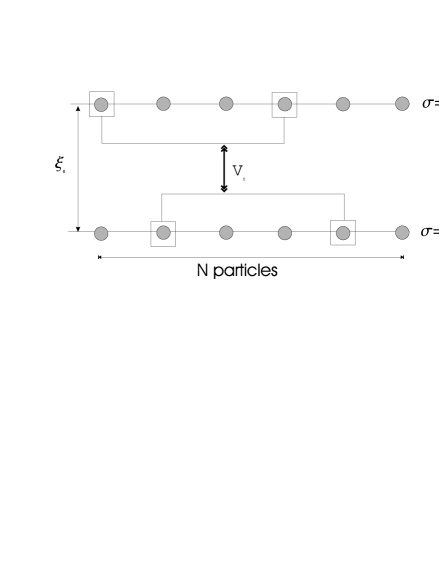
Figure 3.1: The Lipkin model. Note how the interaction only couples states in the lower level to states in the upper level.

The Hamiltonian is

$${\cal H}(\xi_{0},V_{0})=\frac{1}{2}\xi_{0}\sum_{\sigma,p}\sigma a^{\dagger}_{p\sigma}a_{p\sigma}+\frac{1}{2}V_{0}\sum_{pp^{\prime},\sigma}a^{\dagger}_{p\sigma}a^{\dagger}_{p^{\prime}\sigma}a_{p^{\prime}-\sigma}a_{p-\sigma},$$ (3.1)

where $\sigma=\pm 1$ labels the levels (see Fig. 3.1).

A spin representation for $\cal H$ may be found by setting

$$J_{z}=\frac{1}{2}\sum_{p,\sigma}\sigma a^{\dagger}_{p\sigma}a_{p\sigma},\ J_{+}=\sum_{p}a^{\dagger}_{p,+1}a_{p,-1},\ J_{-}=\sum_{p}a^{\dagger}_{p-1}a_{p+1},$$ (3.2)

which satisfy the SU(2) algebra

$$[J_{z},J_{\pm}]=\pm J_{\pm}\;,\;[J_{+},J_{-}]=2J_{z}.$$ (3.3)

The resulting Hamiltonian,

$${\cal H}(\xi_{0},V_{0})=\xi_{0}J_{z}+\frac{1}{2}V_{0}(J_{+}^{2}+J_{-}^{2}),$$ (3.4)

commutes with $J^{2}$ and its irreducible representation breaks up into blocks of size $2j+1$, where $j$ is the total angular momentum quantum number. The low-lyings states occur in the multiplet $j=N/2$ [31], which is a matrix of dimension $N+1$. This is the reason that the model is numerically solvable. Without a quasi-spin representation the dimension of the bare Hamiltonian (3.1) scales exponentially with the number of particles since there are $2^{N}$ basis states, which have the form

$$\prod\nolimits^{N}_{i=1}a_{i\pm}^{+}\left|0\right>.$$ (3.5)

The Hamiltonian (3.4) depends linearly on two parameters. To remove a trivial scaling factor, from now on we divide by $\xi_{0}$ and for convenience drop the prime on the rescaled Hamiltonian (i.e. all our results will be expressed in units of $\xi_{0}$). Defining $\beta_{0}=2jV_{0}/\xi_{0}$ we obtain

$${\cal H}(\beta_{0})=J_{z}+\frac{\beta_{0}}{4j}(J_{+}^{2}+J_{-}^{2}).$$ (3.6)

With no interaction the ground state is the product state of all particles in the lower level $\left|\psi_{0}\right>=\prod\nolimits^{N}_{i=1}a_{i-}^{+}\left|0\right>$ which is written in the spin basis as $\left|\psi_{0}\right>=\left|-j\right>$, and $<\psi_{0}|{\cal H}_{0}|\psi_{0}>=-j$.

3.1.2 Phase transition

The model shows a phase change in the $N\rightarrow\infty$ limit above $\beta_{0}=1$ where the ground state becomes a condensate of pairs, where each pair consists of one particle from the lower level ($\sigma=-1$) and one particle from the upper level ($\sigma=+1$). To see this, we use the Holstein-Primakoff representation of SU(2) to cast the problem in bosonic language,

$$(J_{z})_{B}=-j+b^{\dagger}b,\quad(J_{+})_{B}=(J_{-})^{\dagger}_{B}=b^{\dagger}\sqrt{2j-b^{\dagger}b}.$$ (3.7)

Substituting these into the Hamiltonian (3.6) gives the bosonized version

$${\cal H}_{0}(\beta_{0})=b^{\dagger}b+\beta_{0}(bb+b^{\dagger}b^{\dagger})+O(1/N),$$ (3.8)

where we have also dropped constant terms. Now we perform a standard Bogolubov transformation to rewrite the Hamiltonian (3.8) in terms of new boson operators $B$ and $B^{\dagger}$,

$$b=\cosh\!\phi\,B+\sinh\!\phi\,B^{\dagger},\quad b^{\dagger}=\sinh\!\phi\,B+\cosh\!\phi\,B^{\dagger},$$ (3.9)

where $B$ and $B^{\dagger}$ satisfy $[B,B^{+}]=1$. Choosing $\phi$ so that the $BB$ and $B^{+}B^{+}$ terms vanish gives

$${\cal H}_{0}(\beta_{0})=\sqrt{1-\beta_{0}^{2}}\;B^{\dagger}B+O(1/N)$$ (3.10)

from which we conclude that in the limit $N\rightarrow\infty$, the energy gap $\Delta$ between the ground and first excited states is given by

$$\Delta(\beta_{0})=\left\{\begin{array}[]{r@{\quad\quad}l}\sqrt{1-\beta_{0}^{2}}&\beta_{0}\leq 1\\ 0&\beta_{0}>1\end{array}\right..$$ (3.11)

clearly showing a non-analytic phase transition at $\beta_{0}=1$.

3.2 Some preliminary numerics

3.2.1 Brute force diagonalization

In order to make completely clear the dynamics behind the model, and eliminate any possible confusion that may be lingering in the reader’s mind at this point, we present numerical results for the ground state energy $E_{0}$ and the band gap $\Delta$, as functions of $\beta_{0}$ in Fig. 3.2 and Fig. 3.3. These were obtained by numerical diagonalization routines in the case of $N=50$ particles, so that the $j=N/2$ multiplet is a matrix of dimension $51$. It is clear that there is a sharp change in the nature of the ground state, and in the value of the band gap, around the phase transition line $\beta_{0}=1$. This is made explicit by diagrams of the ground state for two representative $\beta_{0}$ values. These diagrams are to be understood as the components of the ground state $\left<m|\Psi\right>$. In the first phase the ground state has almost all particles on the lower level (i.e. $m=-j$ amplitude is dominant), with only a few excitations. In the second (deformed) phase the ground state is a condensate of pairs (i.e. values of $m$ around zero are dominant). It is important to note that there are no components of the ground state for $m=-j+i$, where $i$ is odd, since the dynamics of the model only promotes/demotes particles in pairs.

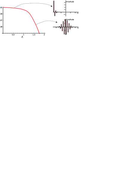
Figure 3.2: Exact ground state energy and its associated state, as a function of $\beta_{0}$, for $N=50$ particles.

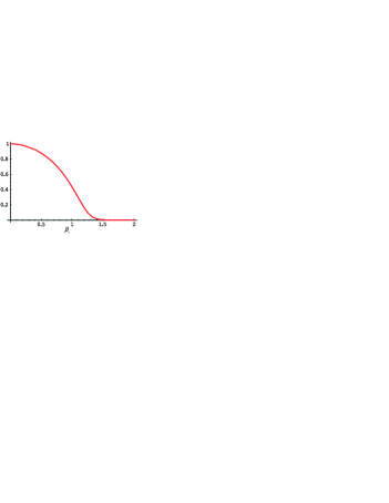
Figure 3.3: Band gap $E_{1}-E_{0}$ as a function of $\beta_{0}$, for $N=50$ particles.

3.2.2 Exact numerical solution of flow equations

The exact solution for the flow equations in certain important cases will now be obtained numerically. This exercise is highly instructive as it shows which operators are important during the flow, as a function of the interaction $\beta_{0}$.

Choice of generator

The first step is to choose a parametrisation of ${\cal H}(\ell)$ that is closed under the flow. The answer to this question depends largely on the choice of generator $\eta(\ell)$. In this model we are interested in the energy spectrum and thus we want to completely diagonalize the Hamiltonian, and not just reduce it into block-diagonal form. Now the operator $X$ in

$$\eta(\ell)=[X,{\cal H}(\ell)]$$ (3.12)

represents the destination of the steepest descent flow (see Chapter 1.3). This presents us with two natural choices:

1. $X=\mbox{Diag}\left({\cal H}(\ell)\right)$ - the original Wegner prescription, or

2. $X=J_{z}$,

both of which will ensure flow to diagonality (the former slightly faster). To make our decision we appeal to the form of the original Hamiltonian (3.6), which is band diagonal (see Fig. 3.4). By “band diagonal” we mean that there are only three bands of nonzero entries in the matrix:

$${\cal H}_{ij}=0\mbox{ unless }i=j\mbox{ or }i=j\pm 2.$$ (3.13)

Figure 3.4: The matrix elements $\left<i\right|H_{0}\left|j\right>$ are zero except for $i=j$, $i=j\pm 2$.

We shall employ the second option and choose our generator as

$$\eta(\ell)=[J_{z},{\cal H}(\ell)]\quad\eta_{ij}=(i-j){\cal H}_{ij}$$ (3.14)

since, contrary to $\eta=[\mbox{Diag}({\cal H}),{\cal H}]$ , this choice preserves the band-diagonal structure of the Hamiltonian. This can be proved directly from multiplying out the types of matrices involved [40]. A more illuminating procedure is to show that the following parametrization of ${\cal H}(\ell)$

$${\cal H}(\ell)=\sum_{\mbox{\scriptsize odd }i}\lambda_{i}(\ell)J_{z}^{i}+\sum_{i}\chi_{i}(\ell)(J_{z}^{i}J_{+}^{2}+J_{-}^{2}J_{z}^{i})$$ (3.15)

remains closed after utilizing (3.14) as the generator. This is the most general matrix of band-diagonal form, as defined above, except that no even powers of $J_{z}$ need be included. The reason for this is as follows. The initial Hamiltonian (3.6) can be rewritten in terms of the $J_{x}$ and $J_{y}$ angular momentum operators

$$J_{x}=\frac{1}{2}(J_{+}+J_{-}),\,J_{y}=\frac{1}{2i}(J_{+}-J_{-})$$ (3.16)

in the following way,

$${\cal H}(\beta_{0})=J_{z}+\frac{\beta_{0}}{2j}(J_{x}^{2}-J_{y}^{2}).$$ (3.17)

The rotational symmetry operation

$$J_{x}\rightarrow J_{y},\,J_{y}\rightarrow J_{x},\,J_{z}\rightarrow-J_{z}$$ (3.18)

transforms ${\cal H}_{0}$ into $-{\cal H}_{0}$, so if $E$ is an eigenvalue of $H_{0}$, then so is $-E$. Consequently the eigenvalues must occur in positive/negative pairs symmetrically situated around the zero point energy. In this way we see that no even powers of $J_{z}$ need be included in (3.15), as such terms would shift the center of the eigenspectrum positively, away from zero, violating the initial symmetry shown in Eq. (3.17).

To show that the parametrisation (3.15) remains closed we consider substituting it into the flow equation $\frac{d{\cal H}}{d\ell}=[[J_{z},{\cal H}],{\cal H}]$. Since the commutator of $J_{z}$ with a power of $J_{\pm}$ takes the schematic form

$$[J_{z},J_{\pm}^{i}]=f_{i}^{\pm}(J_{z})J_{\pm}^{i},$$ (3.19)

where $f_{i}^{\pm}$ is some computable function of $J_{z}$, we see that no new terms will be generated during the flow. In this way the problem has been simplified as the flow has been restricted only to the band-diagonal matrix elements.

Numerical results

Let us first tidy up things by normalizing the diagonal coefficients (powers of $J_{z}$) to the scale of $J_{z}$, and the off-diagonal coefficients to the scale of $J_{+}^{2}+J_{-}^{2}$:

$${\cal H}(\ell)=\sum_{\mbox{\scriptsize odd }i}\lambda_{i}(\ell)\frac{||J_{z}||}{||J_{z}^{i}||}J_{z}^{i}+\sum_{i}\chi_{i}(\ell)\frac{||J_{+}^{2}+J_{-}^{2}||}{||J_{z}^{i}J_{+}^{2}+J_{-}^{2}J_{z}^{i}||}(J_{z}^{i}J_{+}^{2}+J_{-}^{2}J_{z}^{i}).$$ (3.20)

The idea is to get a feeling for the path of the Hamiltonian through operator space. The normalization employed above attempts to eliminate artificial effects due to some of the operators in the basis having larger matrix elements than the others.

The next step is to numerically integrate the flow equation

$$\frac{d{\cal H}}{d\ell}=[[J_{z},{\cal H}],{\cal H}],\quad{\cal H}(0)={\cal H}_{0}(\beta_{0})=J_{z}+\frac{\beta_{0}}{4j}(J_{+}^{2}+J_{-}^{2}).$$ (3.21)

Since the matrices are $N+1$ dimensional, this may be viewed as a set of $N+1+N-1=2N$ nonlinear coupled ordinary differential equations in the diagonal matrix elements $\varepsilon_{i}$ and the two-off-the-diagonal matrix elements $b_{i}$, of the form

$$\dot{\varepsilon}_{i} = 4(b_{i-2}^{2}-b_{i}^{2})$$ (3.22)

$$\dot{b}_{i} = 2b_{i}(\varepsilon_{i}-\varepsilon_{i+2}).$$ (3.23)

After integrating these equations numerically, we perform a change of variables to $\lambda_{i}$ and $\chi_{i}$, to make it clear which operators are excited during the flow. The results are graphed in Fig. 3.5 and Fig. 3.6. In this plot we chose $N=20$ particles, a number large enough to show the general trend but small enough to discriminate meaningfully between the operators.

Fig. 3.5(a) informs us that the powers of $J_{z}$ which constitute the final Hamiltonian $\cal H(\infty)$ are very different in the two phases. In the first phase ($\beta_{0}<1$) the final Hamiltonian is completely dominated by $J_{z}$, while in the second phase ($\beta_{0}>1$) it is dominated by the high powers of $J_{z}$, which occur with large coefficients. Fig. 3.5(b) graphs the path of the Hamiltonian through operator space for $\beta_{0}=1$, the phase change line. The initial part of the flow is characterized by a gradual increase in $J_{z}$, and it is only later that the flow direction changes, and the higher powers of $J_{z}$ are excited. This is a good illustration of the $\ell$-dependency of the generator, and the non-linear nature of the flow equations.

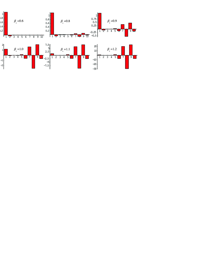
(a) Powers of $J_{z}$ in ${\cal H}(\infty)$

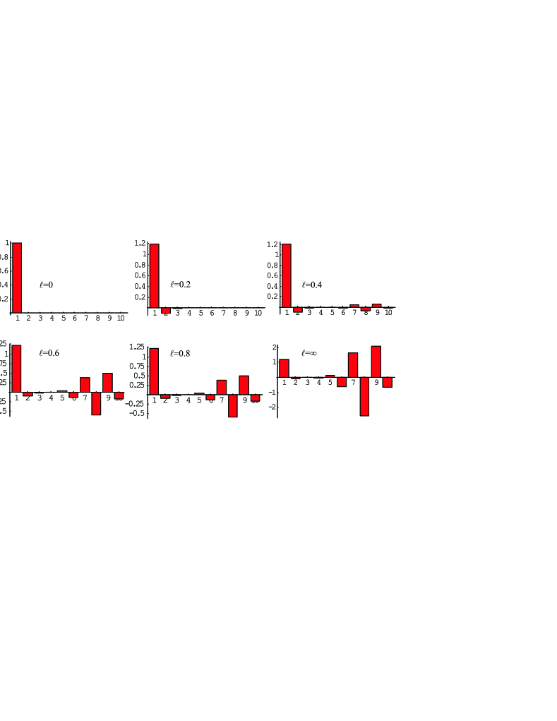
(b) Flow of different powers of $J_{z}$ for $\beta_{0}=1.0$

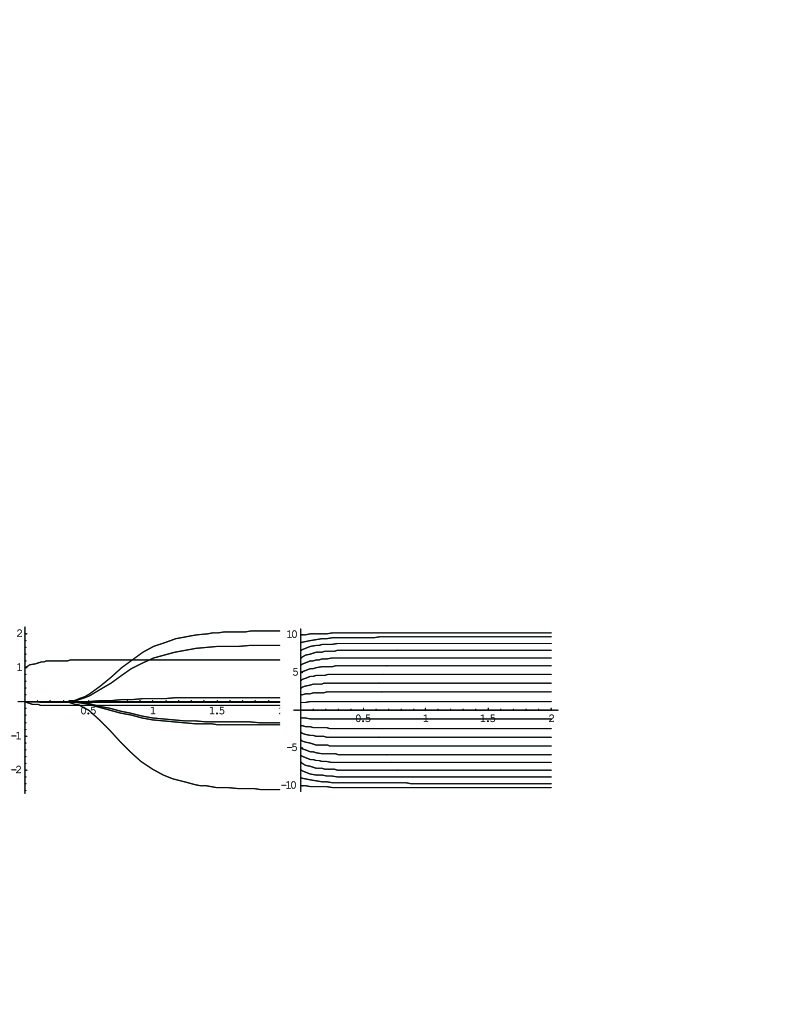
(c) Flow of powers of $J_{z}$ (left) vs flow of diagonal matrix elements (right) for $\beta_{0}=1.0$

Figure 3.5: The powers of $J_{z}$ present for various coupling strengths $\beta_{0}$ and stages $\ell$ during the flow, for $N=20$ particles. The numbers $1\ldots 10$ label the powers of $J_{z}$. Only odd powers need be considered.

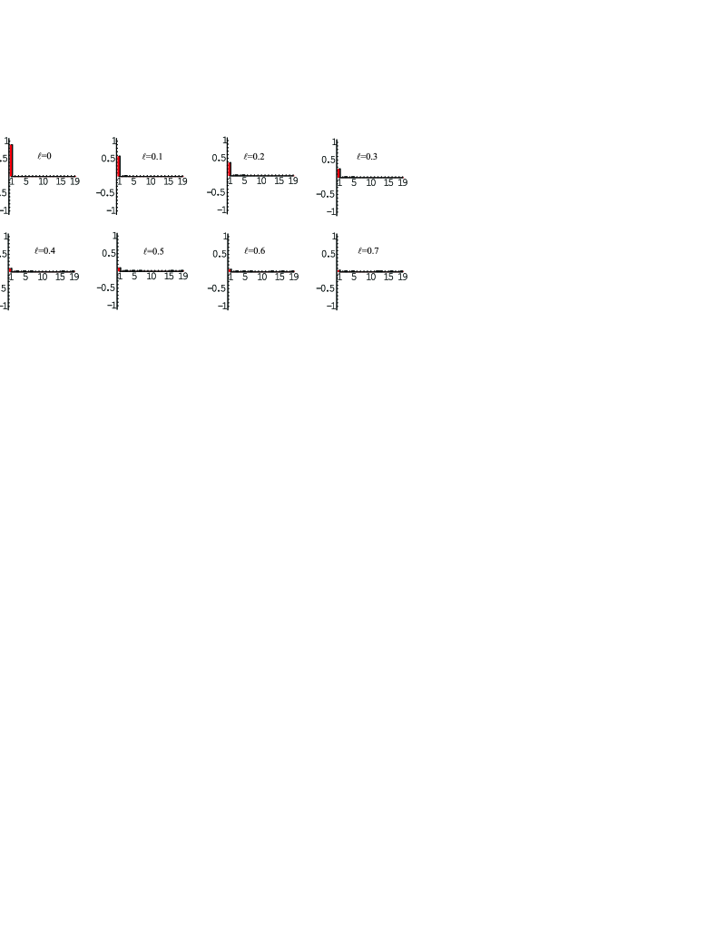
(a) $\beta_{0}=0.9$

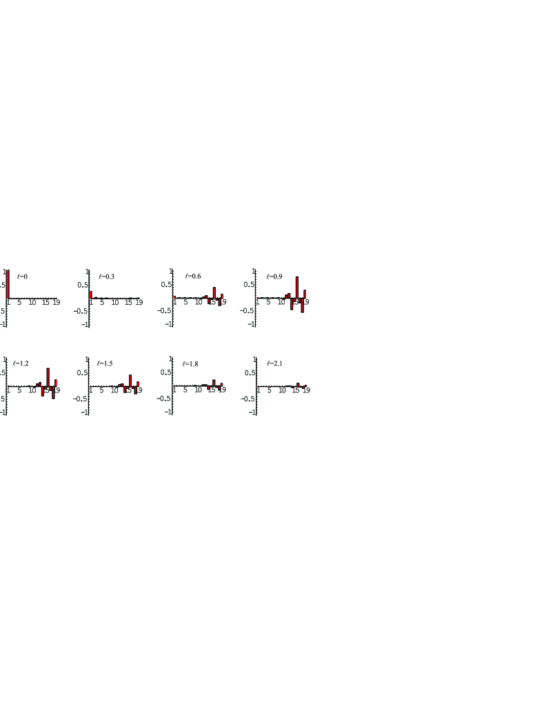
(b) $\beta_{0}=1.1$

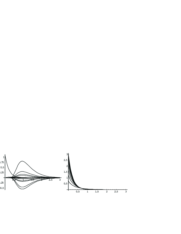
(c) Flow of ${\cal H}_{\mbox{\scriptsize off-diagonal}}$ in $J_{z}$ basis (left) and in terms of actual matrix elements (right) for $\beta_{0}=1.1$

Figure 3.6: Flow of ${\cal H}_{\mbox{\scriptsize off-diagonal}}$ for (a) $\beta_{0}=0.9$ and (b) $\beta_{0}=1.1$. The numbers $1\ldots 20$ label the powers of $J_{z}$ in $(J_{z}^{i}J_{+}^{2}+J_{-}^{2}J_{z}^{i})$. Figure (c) contrasts flow in two different bases.

Fig. 3.5(c) contrasts the flow in the powers of $J_{z}$ basis ($\lambda_{i}$) with the flow of the actual matrix elements ($\varepsilon_{i}$). The former shows the different regimes of the flow referred to above. It is clear that the transformation between the two is “highly geared” since a small change in the matrix elements basis may manifest itself as a large change in the powers of $J_{z}$ basis. Notice again how only the odd powers of $J_{z}$ participate in the flow.

The same analysis is done for the flow of the off-diagonal elements in Fig. 3.6. Since the final Hamiltonian is always diagonal, we have concentrated here on the flow of the off-diagonal elements for two values of the interaction parameter on either side of the phase change boundary, $\beta_{0}=1.0\pm 0.1$. For $\beta_{0}=0.9$ the $J_{+}^{2}+J_{-}^{2}$ term is by far the dominant term in the flow and decreases to zero very quickly, with the higher order terms $J_{z}^{i}J_{+}^{2}+J_{-}^{2}J_{z}^{i}$ hardly participating. For $\beta_{0}=1.1$ the first section of the flow is again dominated by the decrease of $J_{+}^{2}+J_{-}^{2}$, but later on in the flow the higher order terms are highly excited, until they eventually flow to zero too.

This process is made explicit in Fig. 3.6(c), which, similarly to Fig. 3.5(c), contrasts the off-diagonal flow in the $J_{z}^{i}J_{+}^{2}+J_{-}^{2}J_{z}^{i}$ basis ($\chi_{i}$) with the flow of the actual off-diagonal matrix elements ($b_{i}$), for $\beta_{0}=1.1$. It is important to note the distinction that, while the actual matrix elements must decrease monotonically from the analysis presented in Section 1.1, various operator terms may be excited during the flow.

After this preliminary numerical exercise, there should hopefully be no confusion left in the readers minds as to the flow equations program. It has also become clear that the problem will be far more difficult to handle in the second phase, where the flow displays its non-linear behaviour and enlists a range of higher order operators as it evolves. With this in the back of our minds, let us now review some recent treatments of the Lipkin model using flow equations.

3.3 Pirner and Friman’s treatment

Pirner and Friman were the first to apply flow equations to the Lipkin model [38]. Their method was to deal with unwanted newly generated operators by linearizing them around their ground state expectation value. There are two schemes, the second more sophisticated than the first in that it includes a new operator into the flow. The idea, as always, is not to try to solve the Lipkin model (this can be done numerically) or even to try to solve the flow equations in the Lipkin model exactly (this was done in Section 3.2). Rather, one is more interested in finding an effective Hamiltonian for the lower lying states, in such a way that shows promise for application to other systems.

3.3.1 First scheme

The first step is to choose a parametrisation of the flow. For the first scheme we will employ

$${\cal H}(\ell) = \alpha(\ell)J_{z}+\beta(\ell)\frac{1}{4j}(J_{+}^{2}+J_{-}^{2})+\delta(\ell)j$$ (3.24)

$$\alpha(0) = 1$$ (3.25)

$$\beta(0) = \beta_{0}$$ (3.26)

$$\delta(0) = 0,$$ (3.27)

which simply makes the couplings in front of the original Hamiltonian (3.6) $\ell$-dependent. In addition a $\delta$ term proportional to the identity, normalized to the scale of $\alpha$, has been included. In the exact case such a term is never present in the flow since it would shift the centre of the eigenspectrum away from zero. However, an approximation that will be made later will generate such a term(see Eq. (3.31)), and it is necessary if we want to compute the ground state energy. It was not included in the original Pirner and Friman treatment where they were only interested in the gap $\Delta$ between the ground state and the first excited state. We have inserted it here for completeness.

Linearizing newly generated operators

We now employ the generator choice (3.14) in the flow equations. That is, we attempt to solve the differential equation

$$\frac{d{\cal H}(\ell)}{d\ell}=[[J_{z},{\cal H}(\ell)],{\cal H}(\ell)],\;{\cal H}(0)={\cal H}_{0}(\beta_{0}).$$ (3.28)

The first commutator $\eta(\ell)=[J_{z},{\cal H}(\ell)]$ gives

$$\eta(\ell)=\frac{\beta(\ell)}{2}(J_{+}^{2}-J_{-}^{2}).$$ (3.29)

Inserting the Hamiltonian (3.24) into the flow equation (3.28) yields

$$[[Jz,{\cal H}(\ell)],{\cal H}(\ell)]=\beta^{2}\frac{2j(j+1)-1}{4j^{2}}J_{z}-\beta^{2}\frac{1}{2j^{2}}J_{z}^{3}-4\alpha\beta\frac{1}{4j}(J_{+}^{2}+J_{-}^{2}),$$ (3.30)

in which a term $\sim J_{z}^{3}$ has been generated. This generation of ever new operators during the flow is a generic feature of the flow equations; indeed to fully capture the flow we must use many more parameters in the Hamiltonian as in Eq. (3.15). Pirner and Friman dealt with such operators by linearizing them around the ground state expectation value, and neglecting higher-order fluctuations:

$$J_{z}^{3}\mapsto 3\langle J_{z}\rangle^{2}J_{z}-2\langle J_{z}\rangle^{3}.$$ (3.31)

In this way we aim to provide an effective theory for the low-lying states, where the approximation (3.31) is most valid. If we are interested only in the ground state energy, then there is a more accurate linearisation scheme (see Appendix LABEL:LinApp). In the present case we are interested also in properties like the band gap $\Delta$ between the first excited state and the ground state, which makes the linearization (3.31) the best choice. Notice that the term $-2\langle J_{z}\rangle^{3}$ on the RHS of (3.31) has generated a term proportional to the identity, as promised earlier. The presence of this term attests to the fact that we are finding an effective Hamiltonian for the lower lying states, and hence our window must be ‘displaced’ from zero in order to center on the ground state.

It is clear that some further approximation must be employed to evaluate the expectation value in the linearization (3.31), since the ground state is unknown. In Pirner and Friman’s treatment, the expectation value of $J_{z}$ was evaluated with respect to the zero interaction ground state, that is $\left|\Psi\right>=\left|-j\right>$ which gives

$$\left<J_{z}\right>=-j.$$ (3.32)

Substituting the approximation (3.31) into the double commutator (3.30) yields

$$\dot{\alpha} = -\beta^{2}(\frac{6\left<J_{z}\right>^{2}-2j(j+1)+1}{j^{2}})$$ (3.33)

$$\dot{\beta} = -4\alpha\beta$$ (3.34)

$$\dot{\delta} = 4\beta^{2}\frac{\left<J_{z}\right>^{3}}{j^{3}}.$$ (3.35)

The second equation implies that the magnitude of the off-diagonal matrix element $\beta$ decreases in the course of the evolution, providing $\alpha$ remains positive. These equations may easily be combined to give two invariants of the evolution:

$$\delta=(\alpha-1)\frac{4j^{2}}{4j^{2}-2j+1}\,,\qquad\alpha^{2}-\beta^{2}\frac{4j^{2}-2j+1}{4j^{2}}=1-\beta_{0}^{2}\frac{4j^{2}-2j+1}{4j^{2}}.$$ (3.36)

The $j$ dependent terms approach unity for large $j$ (large $N$).

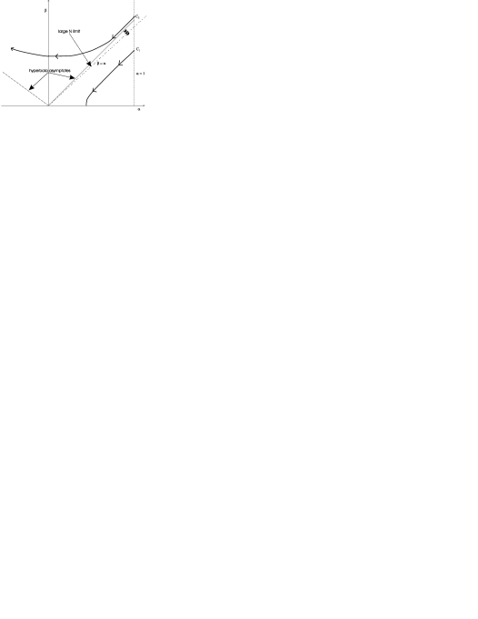
Figure 3.7: The flow of the Hamiltonian parameters in the $\alpha$-$\beta$ plane for the first scheme.

Since $\delta$ is related to $\alpha$ in a simple way, it is instructive to consider the projection of the flow on the $\alpha$-$\beta$ plane. This is illustrated in Fig. 3.7. The Hamiltonian begins at the point $(1,\beta_{0})$. Providing $\beta_{0}<\sqrt{\frac{4j^{2}}{4j^{2}-2j+1}}\sim 1$, as in $C_{1}$, it flows down the hyperbola (3.36), thereby reducing the off-diagonal $\beta$ term to zero and asymptotically intercepting the $\alpha$ axis at $(\alpha(\infty),0)$. If $\beta_{0}>\sqrt{\frac{4j^{2}}{4j^{2}-2j+1}}\sim 1$, as in $C_{2}$, flow occurs along the other branch of the hyperbola and diverges to infinity. This failure of the linearization approximation (3.31) and the expectation value approximation (3.32) will be discussed later. For the first phase the final Hamiltonian is of the form

$${\cal H}(\infty)=\alpha(\infty)J_{z}+j\delta(\infty),$$ (3.37)

which gives the expressions for the ground state energy $E_{0}$ and the gap $\Delta$, for large $N$, as

$$E_{0} = \left<-j\right|{\cal H}(\infty)\left|-j\right>$$ (3.38)

$$= \frac{-4j^{3}+j(2j-1)\sqrt{1-\beta_{0}^{2}(1-\frac{2j-1}{4j^{2}})}}{2j(2j-1)+1}$$ (3.39)

$$\Delta = \left<-j+1\right|{\cal H}(\infty)\left|-j+1\right>-\left<-j\right|{\cal H}(\infty)\left|-j\right>$$ (3.40)

$$= \sqrt{1-\beta_{0}^{2}\frac{4j^{2}-2j+1}{4j^{2}}}$$ (3.41)

$$\approx \sqrt{1-\beta_{0}^{2}}\qquad\mbox{(large $j$)},$$ (3.42)

where the gap $\Delta$ agrees with the exact result (3.11) in the large $N$ limit.

3.3.2 Second scheme

In the second scheme we attempt more accuracy by including a $J_{z}^{3}$ term in our parametrization of the Hamiltonian:

$${\cal H}(\ell)=\alpha(\ell)J_{z}+\gamma(\ell)\frac{1}{j^{2}}J_{z}^{3}+\beta(\ell)\frac{1}{4j}(J_{+}^{2}+J_{-}^{2})$$ (3.43)

$$\alpha(0)=1,\quad\gamma(0)=0,\quad\beta(0)=\beta_{0}.$$ (3.44)

The $\delta$ identity term has been dropped as our linearization scheme will not generate such a term. Substitution into the double bracket commutators of the flow equations will yield the same generator (3.45), since $J_{z}^{3}$ commutes with $J_{z}$:

$$\eta(\ell)=\frac{\beta(\ell)}{2}(J_{+}^{2}-J_{-}^{2}).$$ (3.45)

For the second commutator we will be faced with evaluating

$$[J_{+}^{2}-J_{-}^{2},J_{z}^{3}].$$ (3.46)

However, applying our rule $J_{z}^{3}\rightarrow 3\left<J_{z}\right>^{2}J_{z}-2\left<J_{z}\right>^{3}$ does not commute with applying the commutator:

$$[\cdot,\cdot]\circ\mbox{linearize} \rightarrow -6\left<J_{z}\right>^{2}(J_{+}^{2}+J_{-}^{2})$$ (3.47)

$${}\mbox{linearize}\circ[\cdot,\cdot] \rightarrow \left(12(1-\left<J_{z}\right>)J_{z}+6\left<J_{z}\right>^{2}-8\right)J_{+}^{2}+conj.$$ (3.48)

The operators are understood to be applied from right to left, as is conventional. We choose to linearize first, as Pirner and Friman did. Linearizing second generates additional off-diagonal terms. This point will be discussed later in Section 3.6. As promised, in either case no term proportional to the identity is generated. An interesting difference with the first scheme is that in the second scheme the approximation $J_{z}^{3}\rightarrow 3\left<J_{z}\right>^{2}J_{z}-2\left<J_{z}\right>^{3}$ gets tagged with the off-diagonal elements while in the first scheme it gets tagged with the diagonal elements. The flow equations are

$$\dot{\alpha} = \beta^{2}\left(\frac{2j(j+1)-1}{j^{2}}\right)$$ (3.49)

$$\dot{\beta} = -4\left(\alpha\beta+\frac{3\beta\gamma\left<J_{z}\right>^{2}}{j^{2}}\right)$$ (3.50)

$$\dot{\gamma} = -2\beta^{2}.$$ (3.51)

Combining the first and third equations gives

$$\gamma=\frac{2j^{2}}{2j(j+1)-1}(1-\alpha).$$ (3.52)

Eliminating $\gamma$ gives rise to another more complicated invariant

$$(4k-24)\alpha^{2}+48\alpha+k^{2}\beta^{2}=4k+24+k^{2}\beta_{0}^{2},$$ (3.53)

where

$$k=\frac{2j(j+1)-1}{j^{2}}\rightarrow 2\mbox{ (large j)}.$$ (3.54)

The invariant (3.53) may be interpreted as a shifted hyperbola by setting $\bar{\alpha}=\alpha-\frac{24}{24-4k}$

$$(24-4k)^{2}\bar{\alpha}^{2}-(24-4k)k^{2}\beta^{2}=4k^{3}\beta_{0}^{2}-24k^{2}\beta_{0}^{2}+16k^{2}.$$ (3.55)

The asymptotes of this hyperbola are given by the lines

$$\beta_{\mbox{\scriptsize asymptotes}}^{(2)}=\pm\left(-2\frac{6-k}{k^{2}}\alpha+\frac{12}{\sqrt{6-k}\,k^{2}}\right)\rightarrow\pm\left(-2\alpha+3\right)\mbox{ (large j)}.$$ (3.56)

The analysis runs similarly as before, and the flow in the $\alpha$-$\beta$ plane is illustrated in Fig. 3.8. It begins at $(1,\beta_{0})$, but this time $\alpha$ is set to increase. Providing

$$\beta_{0}<\beta_{\mbox{\scriptsize asymptotes}}^{(2)}(1)=\frac{2j}{\sqrt{4j^{2}-2j+1}}\rightarrow 1\mbox{ (large $j$)},$$ (3.57)

as in ${\cal C}_{1}$, the Hamiltonian flows down the lower branch of the hyperbola,

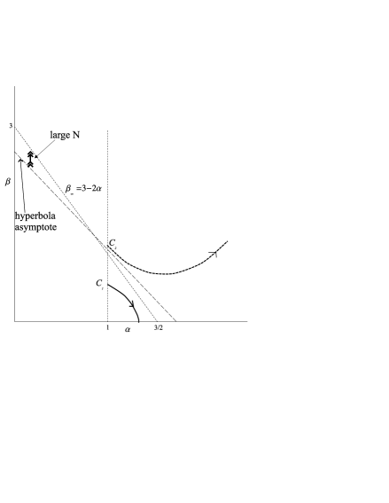
Figure 3.8: The flow of the Hamiltonian parameters in the $\alpha$-$\beta$ plane for the second scheme.

decreasing the off-diagonal term $\beta$, and intercepts the $\alpha$ axis at

$$\alpha(\infty)=\frac{6}{6-k}-\frac{k\sqrt{4-(6-k)\beta_{0}^{2}}}{2(6-k)}.$$ (3.58)

If $\beta_{0}>\frac{2j}{\sqrt{4j^{2}-2j+1}}$ as in ${\cal C}_{2}$, the Hamiltonian flows along the upper hyperbola and diverges to infinity.

In the first phase, the final Hamiltonian is of the form

$${\cal H}(\infty)=\alpha(\infty)J_{z}+\gamma(\infty)\frac{1}{j^{2}}J_{z}^{3},$$ (3.59)

which together with the $\alpha$-intercept (3.58) and the $\gamma$ invariant (3.52) gives

$$E_{0} = \frac{-4j^{3}+j(2j-1)\sqrt{1-\beta_{0}^{2}(1-\frac{2j-1}{4j^{2}})}}{2j(2j-1)+1}$$ (3.60)

$$\Delta = \left((-j+1)\alpha(\infty)+{\frac{(-j+1)^{3}}{j^{2}}}\gamma(\infty)\right)-\left(-j\alpha(\infty)+{\frac{-j^{3}}{j^{2}}}\gamma(\infty)\right)$$ (3.61)

$$= \frac{6j-2+(4j(j-2)+3)\sqrt{1-\beta_{0}^{2}\left(1-\frac{2j-1}{4j^{2}}\right)}}{2j(2j-1)+1}$$ (3.62)

$$\approx \sqrt{1-\beta_{0}^{2}}\mbox{ (large $j$)}.$$ (3.63)

The result for the ground state is the same as in the first scheme (3.39). Due to the $J_{z}^{3}$ term, the new gap (3.62) differs from the previous result (3.41).

3.3.3 Discussion

At this stage it is instructive for purposes of comparison to consider an exact power series expansion of the ground state energy in the coupling $\beta_{0}$. Only even powers of $\beta_{0}$ will appear due to the symmetry of the Hamiltonian (as explained underneath Eq. (3.15) . To fourth order, the result from perturbation theory is [31]

$$E_{0}^{\mbox{ex}}(\beta_{0},j)=-j+\frac{1}{8}(\frac{1}{j}-2)\beta_{0}^{2}-\-\frac{(2j-1)(4j^{2}-14j+9)}{32j^{3}}\beta_{0}^{4}+\cdots$$ (3.64)

On the other hand, a series expansion of our result (both schemes gave the same value for the ground state energy) gives:

$$E_{0}(\beta_{0},j)=-j+\frac{1}{8}(\frac{1}{j}-2)\beta_{0}^{2}+\frac{(2j-1)(4j^{2}-2j+1)}{128j^{2}}\beta_{0}^{4}+\cdots$$ (3.65)

The flow equations result is correct up to order $\beta_{0}^{2}$. This fact is not entirely trivial since it is not clear precisely how many orders of $\beta_{0}$ are accounted for by the linearization procedure (3.31) and the expectation value approximation (3.32). The fourth order term as a function of $N=2j$ in the exact case and in the flow equations result, for both the ground state energy and the gap energy, are plotted in Fig. 3.9(g) and Fig. 3.9(h). The flow equations result is close to the exact value, but becomes less accurate with increasing particle number.

The results for the ground state energy (3.60), (3.39) and the energy gap (3.41), (3.62) are plotted in Fig. 3.9, where the exact results are also shown. Figs. 3.9(a) and (b) plot the ground state energy, and the gap against $\beta_{0}$, for $N=30$ particles. For small $\beta_{0}$ both schemes deliver accurate results. As $\beta_{0}$ increases to unity, the ground state energy starts to diverge. The gap energy from the second scheme is more accurate than the result in the first scheme.

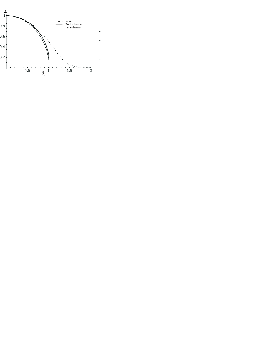
(a) Gap $\Delta$ vs $\beta_{0}$ for $N=30$ particles.

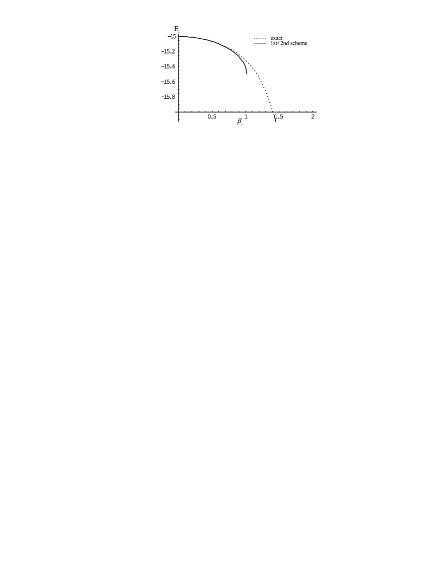
(b) Ground state $E_{0}$ vs $\beta_{0}$ for $N=30$ particles.

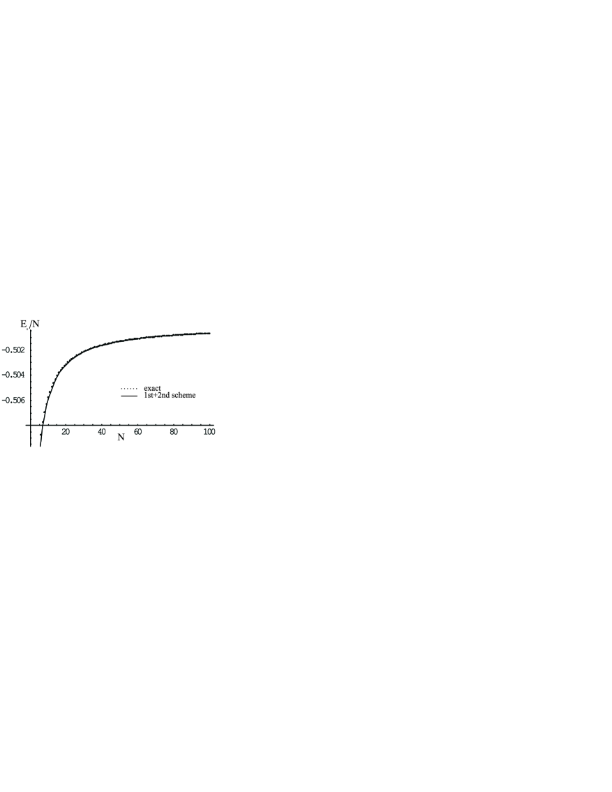
(c) Ground state energy per particle vs $N$. $\beta_{0}=0.5$.

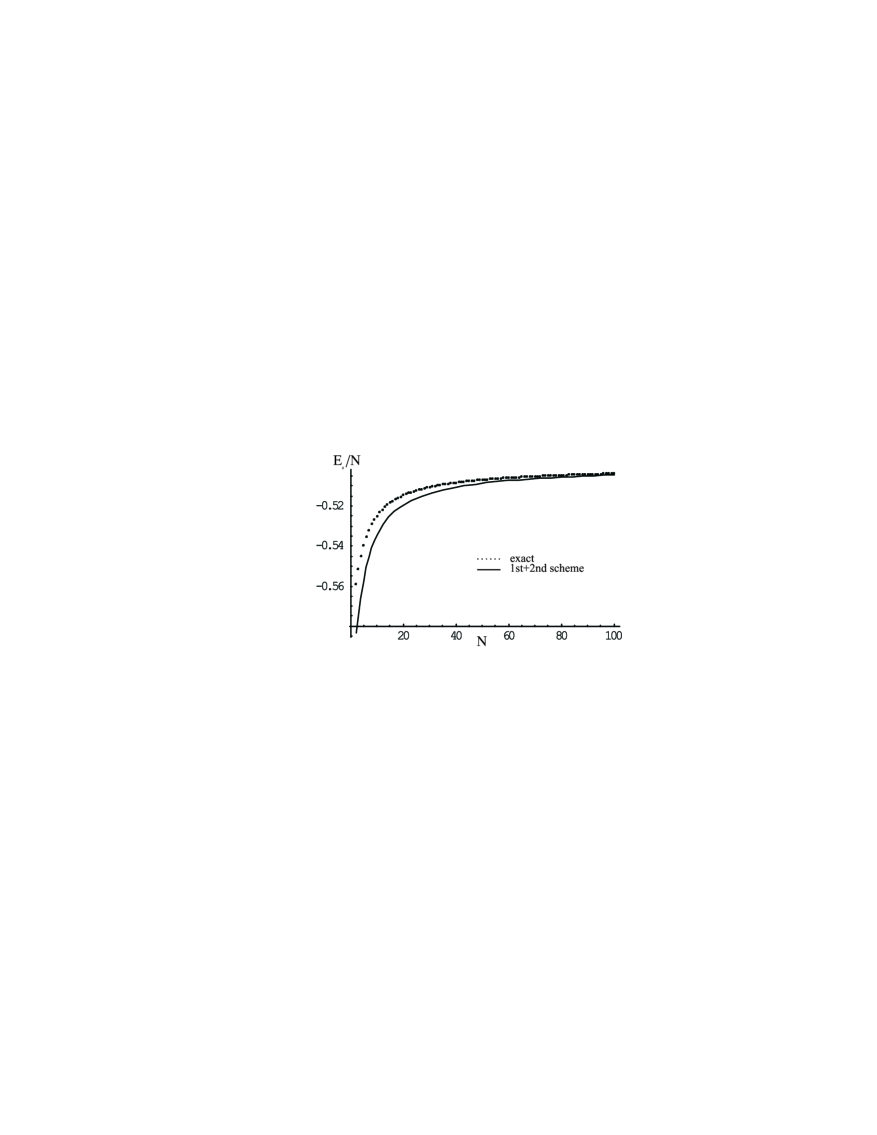
(d) Ground state energy per particle vs $N$. $\beta_{0}=1.0$.

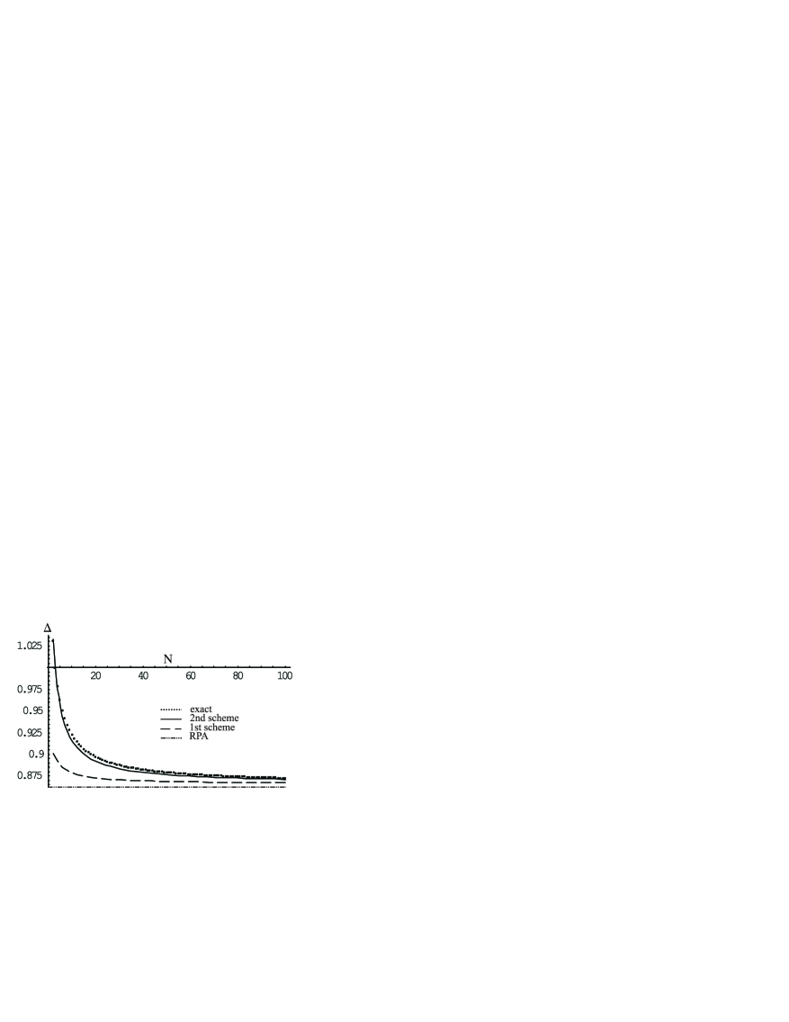
(e) Gap $\Delta$ vs $N$. $\beta_{0}=0.5$

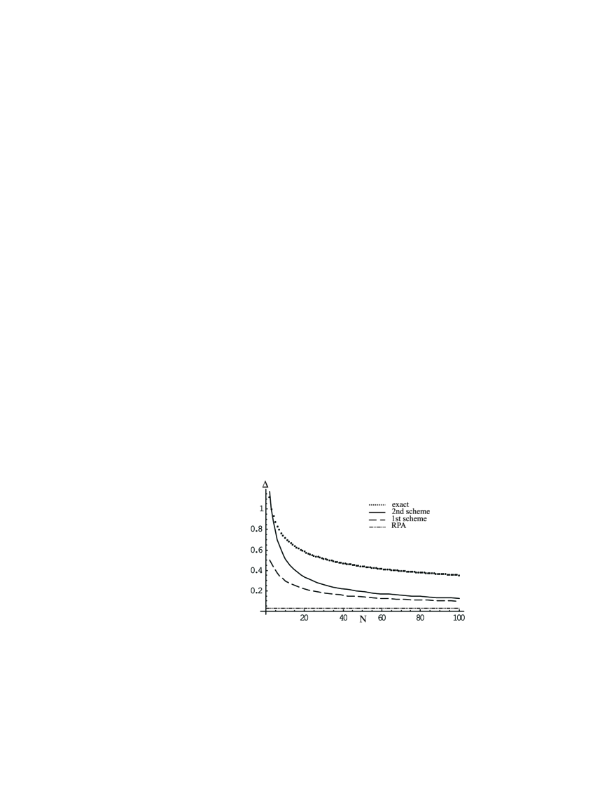
(f) Gap $\Delta$ vs $N$. $\beta_{0}=1.0$

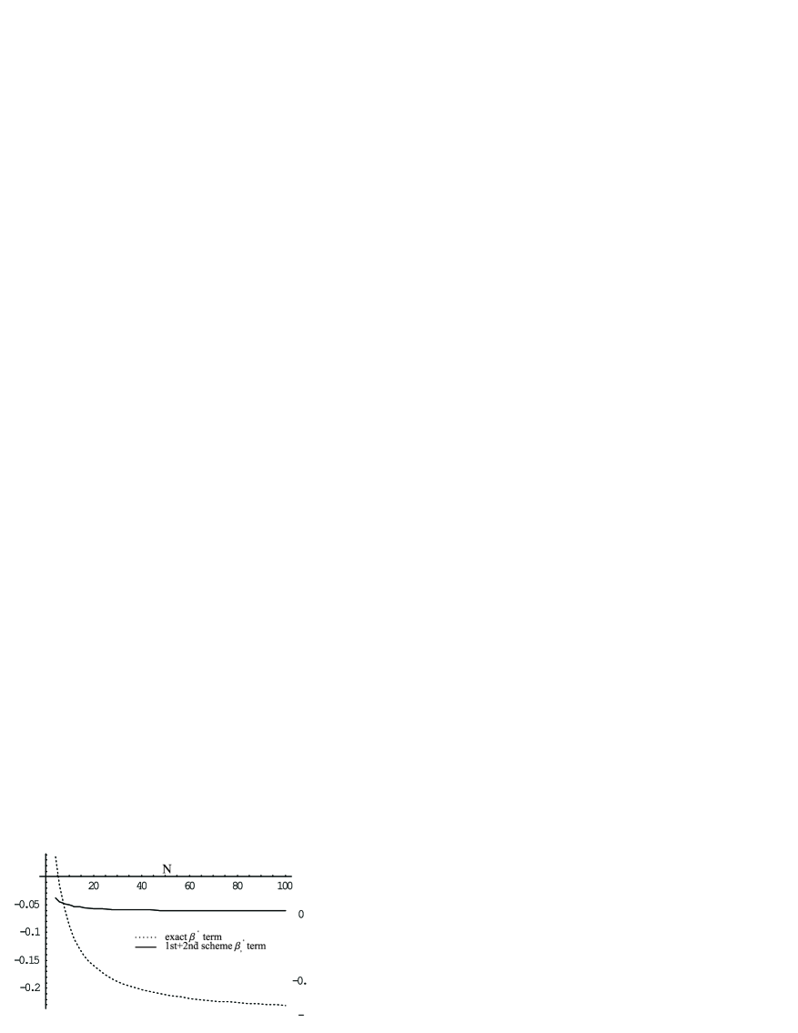
(g) Coefficient of $\beta_{0}^{4}$ for ground state $E_{0}$.

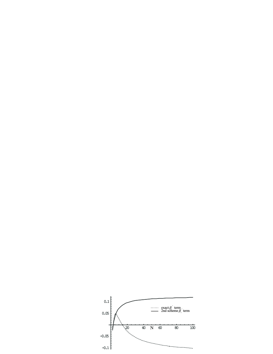
(h) Coefficient of $\beta_{0}^{4}$ for gap $\Delta$.

Figure 3.9: Comparison of exact results and the two flow equations schemes. Both schemes give divergent results in the second phase $\beta_{0}>1$.

This is made more apparent in Figs. 3.9(c)-(f) which plot the behavior of the ground state energy per particle, and the gap, as a function of $N$, for fixed $\beta_{0}$. For comparison the RPA result [32] is also shown. We see that including a $J_{z}^{3}$ term during the flow has considerably improved the accuracy of the method. A perturbative treatment here would require an expansion of the ground state energy as a function of $1/N$, for fixed $\beta_{0}$. This is not possible using ordinary perturbation theory since $1/N$ enters into the Hamiltonian (3.6) in both the coupling and implicitly in the dimensions of the matrices involved. It is here that flow equations have an advantage since they successfully interpolate between perturbation theory for small $N$ and RPA for large $N$ [38]. Indeed, instead of expanding the flow equations result in $\beta_{0}$ as in Eq. (3.65), one may expand it in $1/j$. This exercise gives

$$E_{0}(\beta_{0},j)=-j-\frac{1}{2}(1-\sqrt{1-\beta_{0}^{2}})+\frac{\beta_{0}^{2}}{8\sqrt{1-\beta_{0}^{2}}}\frac{1}{j}+\cdots$$ (3.66)

The failure of the linearisation scheme when $\beta_{0}>1$ is due to the fluctuations in $J_{z}$ becoming stronger, so the expansion of the new operators in powers of fluctuating operators is not so good anymore. This point becomes clearer from examining the powers of $J_{z}$ involved in the flow in the second phase, from Section 3.2.2. Nevertheless, we have developed a simple way to modify the linearisation scheme to be able to deal with this phase, which will be presented in Section 3.6 . For now we continue our review of treatments of the Lipkin model using flow equations.

3.4 Mielke’s matrix element treatment

Dissatisfied with the fact that the original Wegner generator $\eta=[\mbox{Diag}({\cal H}),{\cal H}]$ did not conserve the band structure of a matrix, Mielke proposed in 1998 a new choice of generator [41],

$$\eta_{ij}=\mbox{sign}(i-j){\cal H}_{ij},$$ (3.67)

constructed to ensure that band diagonality is preserved. This choice of generator cannot be written as a commutator of some matrix with ${\cal H}$. The proof that it conserves band diagonality follows from

$$\frac{d{\cal H}_{ij}}{d\ell}=[\eta,{\cal H}]_{ij}=-\mbox{sign}(i-j)({\cal H}_{ii}-{\cal H}_{jj}){\cal H}_{ij}+\sum_{k\neq(n,m)}\left(\mbox{sign}(i-k)+\mbox{sign}(j-k)\right){\cal H}_{ik}{\cal H}_{kj}.$$ (3.68)

If the Hamiltonian is band diagonal (${\cal H}_{ij}=0$ if $|i-j|>M$) then the sum of the sign functions in the second term will vanish for the matrix elements outside the band. Mielke was obviously not aware that precisely this problem had been studied before in the mathematical literature [40], where it was proved that writing the generator as the commutator of ${\cal H}$ with a diagonal matrix with a constant difference between its diagonal elements would conserve band diagonality. In the Lipkin model, $J_{z}$ is an operator with such a property. Indeed,

$$\eta_{ij}=[J_{z},{\cal H}]_{ij}=(i-j){\cal H}_{ij}$$ (3.69)

clearly resembles Mielke’s generator (3.67) and also causes the second term in Eq. (3.68) to vanish. For a matrix with a single band (i.e. only one band other than the diagonal is non-zero), the two choices of generator will differ only by a constant factor. Therefore, rather than discussing Mielke’s generator, we shall focus on his direct method of solving the flow equations for the Lipkin model.

We want to consider the flow equations directly from the matrix elements. The Hamiltonian is

$${\cal H}(\beta_{0})=J_{z}+\frac{\beta_{0}}{4j}(J_{+}^{2}+J_{-}^{2}).$$ (3.70)

Since the interaction only connects $\left|m\right>$ with $\left|m\pm 2\right>$, we now rearrange the basis $\{\left|-j\right>,\left|-j+1\right>,\cdots,\left|+j\right>\}$ into odd and even $m$. For example, for even $N$ we form

$$\{\left|-j\right>,\left|-j+2\right>,\cdots,\left|+j\right>\}\cup\{\left|-j+1\right>,\left|-j+3\right>,\cdots,\left|j-1\right>\}.$$ (3.71)

In this way $\cal H$ splits into two tridiagonal (${\cal H}_{ij}=0$ if $|i-j|>1$) submatrices, the dimension of which depends on $N$. If $N$ is even, one of the matrices has dimension $N/2+1$, and the other $N/2$. If $N$ is odd, both matrices have dimension $\frac{N+1}{2}$. We write the matrix elements as

$$\varepsilon_{n}={\cal H}_{nn},\quad\theta_{n}={\cal H}_{nn+1},\quad n=0\ldots\mbox{Dim}({\cal H}).$$ (3.72)

The initial values are easily computed to be

$$\varepsilon_{n}(0) = -j+2n$$ (3.73)

$$\theta_{n}(0) = \frac{\beta_{0}}{4j}\sqrt{j(j+1)-(j-2n)(j-2n-1)}\sqrt{j(j+1)-(j-2n-1)(j-2n-2)},$$ (3.74)

or

$$\varepsilon_{n}(0) = -j+2n+1$$ (3.75)

$$\theta_{n}(0) = \frac{\beta_{0}}{4j}\sqrt{j(j+1)-(j-2n-1)(j-2n-2)}\sqrt{j(j+1)-(j-2n-2)(j-2n-3)}.$$ (3.76)

Using our generator as $\eta=[J_{z},{\cal H}]$, where ${\cal H}$ is expressed in the rearranged basis, the flow equations are in both cases

$$\frac{d\varepsilon_{n}}{d\ell} = -2(\theta_{n}^{2}-\theta_{n-1}^{2})$$ (3.77)

$$\frac{d\theta_{n}}{d\ell} = -\theta_{n}(\varepsilon_{n+1}-\varepsilon_{n}),$$ (3.78)

which are a simple modification of the direct matrix element equations for the original combined matrix (3.22). The problem is now to solve these equations. As Mielke pointed out, a first possibility is to solve them iteratively, by starting with the ansatz $\varepsilon_{n}^{(0)}(\ell)=\varepsilon(0)$ and $\theta_{n}^{(0)}(\ell)=\theta_{n}(0)e^{-2\ell}$. These expressions could then be inserted onto the right hand side of Eqs. (3.77) and (3.78), which would yield a first iterative solution, which could again be inserted onto the right hand side and so on. This procedure rapidly becomes more complex. It follows the philosophy of perturbation theory, and works well for small $\beta_{0}$ and small $N$. A non-perturbative solution can be obtained in the limit of large $N$, which is the regime we are interested in. The first step is noticing that the off-diagonal matrix elements initially satisfy

$$\theta_{n}(0)^{2}-\theta_{n-1}(0)^{2}=2\beta_{0}^{2}(n+\frac{1}{4})(1+\mbox{O}(1/j))$$ (3.79)

in the first case 3.74, or

$$\theta_{n}(0)^{2}-\theta_{n-1}(0)^{2}=2\beta_{0}^{2}(n+\frac{3}{4})(1+\mbox{O}(1/j))$$ (3.80)

in the second case 3.76. The reason this is important is because this expression is used in the right hand side of the flow equations (3.77). The idea is to use the large $N$ limit to reduce our set of dynamical variables:

$$\underbrace{\{\varepsilon_{n}(\ell),\theta_{n}(\ell)\}}_{\mbox{\scriptsize$N/2+1+N/2-1=N$ variables}}\rightarrow\qquad\underbrace{\{a(\ell),b(\ell),f(\ell)\}}_{\mbox{\scriptsize$3$ variables}}.$$ (3.81)

This is achieved by making the ansatz:

$$\varepsilon_{n}(\ell) = na(\ell)+b_{1,2}(\ell)$$ (3.82)

$$\theta_{n}(\ell) = f(\ell)\theta_{n}(0),$$ (3.83)

where the subscript on $b_{1,2}$ refers to the submatrix being diagonalized. This ansatz attempts to track the flow of the diagonal part of $\cal H$ in a linear fashion. This is illustrated in Fig. 3.10, which also shows for comparison the exact

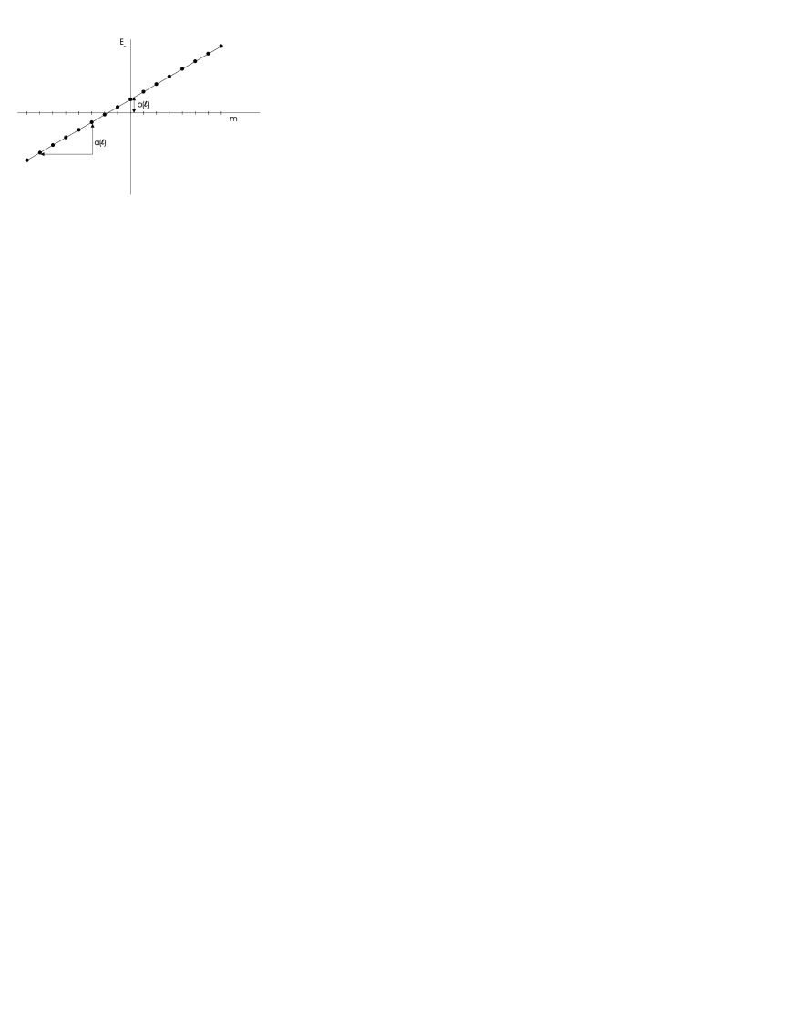
(a)

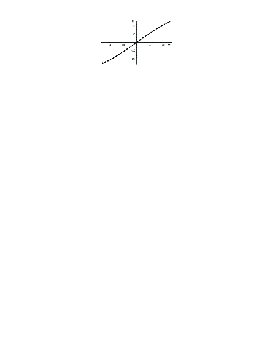
(b)

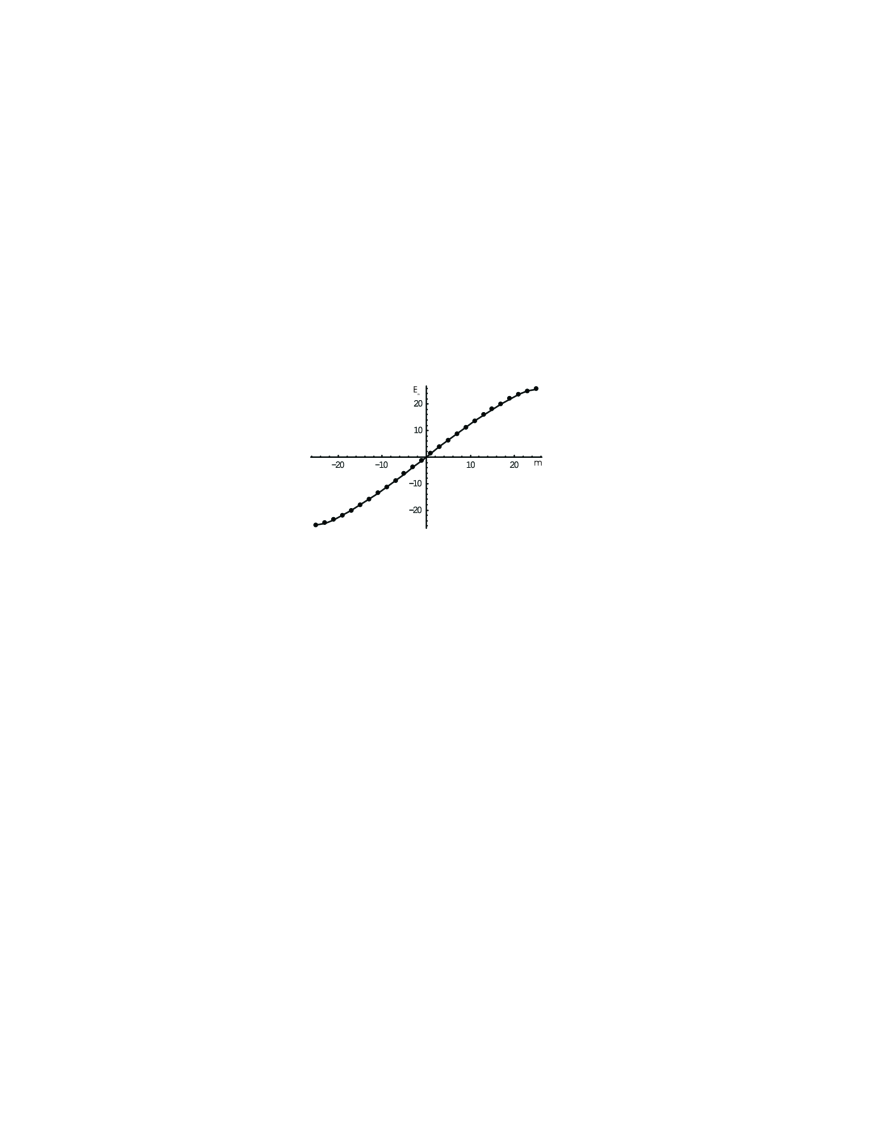
(c)

Figure 3.10: (a) Schematic illustration of ansatz (3.82). (b) Exact spectrum for $\beta_{0}=0.8$. (c) Exact spectrum for $\beta_{0}=1.2$. $N=50$ particles. Note how boundary effects enter for larger $\beta_{0}$.

numerical calculation of the form of the eigenvalues, for the odd $m$ submatrix, with $N=50$ particles and two values of the coupling on either side of the phase boundary, $\beta_{0}=0.8$ and $\beta_{0}=1.2$. This figure shows that the linear ansatz (3.82) should work well in the first phase, but poorly in the second phase where there are boundary effects.

The ansatz (3.82), in the large $N$ limit, leads to the following differential equations for $a$, $b_{1,2}$ and $f$:

$$\frac{df}{d\ell} = -af$$ (3.84)

$$\frac{da}{d\ell} = -4\beta_{0}^{2}f^{2}$$ (3.85)

$$\frac{db_{1}}{d\ell} = \frac{1}{4}\frac{da}{d\ell}\mbox{(using \ref{offs1}),}\qquad\frac{db_{2}}{d\ell}=\frac{3}{4}\frac{da}{d\ell}\mbox{(using \ref{offs2})}$$ (3.86)

$$f(0) = 1,\quad a(0)=2,\quad b_{1}(0)=-j,\quad b_{2}(0)=-j+1.$$ (3.87)

Since the first two equations leave $a^{2}-4\beta_{0}^{2}$ invariant, and since $f\rightarrow 0$ as $\ell\rightarrow\infty$, this yields directly

$$a(\infty)=2\sqrt{1-\beta_{0}^{2}},$$ (3.88)

which, for one thing, shows that the reduction of variables for large $N$, using (3.81), is only valid in the first phase, $\beta_{0}<1$. This result also yields immediately, from the initial conditions (3.87) and the equations (3.86)

$$b_{1}(\infty) = -j-\frac{1}{2}+\frac{1}{2}\sqrt{1-\beta_{0}^{2}}$$ (3.89)

$$b_{2}(\infty) = -j-\frac{1}{2}+\frac{3}{2}\sqrt{1-\beta_{0}^{2}}.$$ (3.90)

In this way the spectrum for large $N$ is given as

$$\varepsilon_{n1,2}=2\sqrt{1-\beta_{0}^{2}}(n+\frac{1}{2}\pm\frac{1}{4})-j-\frac{1}{2},$$ (3.91)

which yields the ground state as

$$E_{0}=\varepsilon_{0,2}=-j-\frac{1}{2}(1-\sqrt{1-\beta_{0}^{2}}),$$ (3.92)

and the gap

$$\Delta=\sqrt{1-\beta_{0}^{2}}.$$ (3.93)

This expression for the gap corresponds to Eq. (3.11), obtained from a Bogolubov transformation. The expression for the ground state verifies the power series obtained from the flow equations previously in Eq. (3.66). Mielke’s direct approach to the flow equations via the matrix elements themselves has readily yielded the correct results for large $N$ in the first phase. Extending the approach to the next order in $1/N$ would require a polynomial ansatz for $\varepsilon_{n}$ as opposed to the linear one in Eq. (3.82), and extending the expression for $\theta_{n}^{2}(0)-\theta_{n-1}^{2}(0)$ to the corresponding power of $1/N$. The complexity of this approach rapidly increases and, although systematic, it cannot be viewed as a miracle method for the $1/N$ expansion of the properties of the model.

3.5 Stein’s bosonization method

Stein [43] has recently employed the flow equations in the Lipkin model by considering the flow in the Holstein-Primakoff boson representation of the angular momentum operators. In this way it is possible to systematically solve the flow to any order in $1/N$. In this section we review his procedure, presenting it in a unified and improved manner.

Since we will be studying properties such as the ground state in the large $N$ limit, we firstly rescale our Hamiltonian to ensure that the ground state energy is of the order of unity : ${\cal H}^{\prime}=\frac{1}{j}{\cal H}$. This means that

$$\frac{d{\cal H}^{\prime}}{d\ell}=\frac{1}{j}\frac{d{\cal H}}{d\ell}=\frac{1}{j}[[J_{z},{\cal H}],{\cal H}]=[[jJ_{z},{\cal H}^{\prime}],{\cal H}^{\prime}],$$ (3.94)

from which it is clear that if we wish to maintain the traditional double bracket form of the flow equations, we must rescale $J_{z}$ by a factor of $j$. Dropping primes in our subsequent work, our by now familiar Hamiltonian reads

$${\cal H}_{0}=\frac{1}{j}J_{z}+\frac{\beta_{0}}{4j^{2}}(J_{+}^{2}+J_{-}^{2}).$$ (3.95)

We now employ the Holstein-Primakoff realization of angular momentum(as in Eq. (3.7))

$$(J_{z})_{B}=-j+a^{\dagger}a,\quad(J_{+})_{B}=(J_{-})^{\dagger}_{B}=\sqrt{2j}a^{\dagger}\sqrt{1-\frac{1}{2j}a^{\dagger}a},$$ (3.96)

where $b^{(\dagger)}$ are bosonic annihilation (creation) operators. Expanding the square root to order $\frac{1}{j^{2}}$ gives

$${\cal H}_{0}=-1+\frac{1}{j}\left(a^{\dagger}a+\frac{\beta_{0}}{2}(1-\frac{1}{4j})(a^{\dagger}a^{\dagger}+aa)\right)-\frac{1}{j^{2}}\frac{\beta_{0}}{4}\left((a^{\dagger}a^{\dagger}a^{\dagger}a+a^{\dagger}aaa)\right)-\cdots$$ (3.97)

where we have announced our intention to normal order all terms, and also to list each operator in the series only once - at that order of $1/j$ where it first appeared. Subsequent generations of the same operator from normal ordering or the flow will be grouped together with the initial one. As the Hamiltonian evolves, we will track it in the following form

$${\cal H}(\ell)=-1+\sum_{k=1}^{\infty}\frac{:{\cal H}^{D}_{k}(\ell)+{\cal H}^{\pm 2}_{k}(\ell):}{j^{k}}.$$ (3.98)

Since we choose $\eta=[jJ_{z},{\cal H}]$ as the generator, the Hamiltonian will remain tridiagonal, or in bosonic language, only contain functions of the number operator (${\cal H}_{k}^{D}$) or operators that change the occupation number by two (${\cal H}_{k}^{\pm 2}$). This point has been confused in Ref. [43] where extra terms were added to the generator for each order of $1/j$ in order to conserve tridiagonality. The choice $\eta=[jJ_{z},{\cal H}]$ produces these extra terms automatically. To be explicit, the flow of ${\cal H}$ up to order $\frac{1}{j^{2}}$ will be parameterized as

$${\cal H}(\ell)=-1+\frac{1}{j}\left(E(\ell)+f(\ell)a^{\dagger}a+\frac{\beta_{0}}{2}g(\ell)(a^{\dagger}a^{\dagger}+aa)\right)+\frac{\beta_{0}}{j^{2}}\left(h(\ell)a^{\dagger}a^{\dagger}aa-\frac{1}{4}\zeta(\ell)(a^{\dagger}a^{\dagger}a^{\dagger}a+a^{\dagger}aaa)\right).$$ (3.99)

Due to our policy of listing each operator only once, the flow coefficients must also be viewed as being $j$ dependent, and hence can be arranged as a power series in $1/j$.

We first compute everything up to order $1/j$. In this case the initial conditions are, from (3.97),

$$f(0)=1,\quad g(0)=1,\quad E(0)=0.$$ (3.100)

The generator is

$$\eta=[ja^{\dagger}a,{\cal H}]=\beta_{0}g(a^{\dagger}a^{\dagger}+aa).$$ (3.101)

The computation of the flow equations commutator yields, to order $1/j$,

$$[\eta,{\cal H}]=\frac{1}{j}\left(-2\beta_{0}^{2}g^{2}-4\beta_{0}^{2}g^{2}a^{\dagger}a-\frac{\beta_{0}}{2}4\beta_{0}fg(a^{\dagger}a^{\dagger}+aa)\right).$$ (3.102)

The identity term arises from the normal ordering of $[a^{\dagger}a^{\dagger}-aa,a^{\dagger}a^{\dagger}+aa]$, and is not generated in higher orders. Comparison with the Hamiltonian (3.99) gives

$$\frac{df}{d\ell} = -4\beta_{0}^{2}g^{2}$$ (3.103)

$$\frac{dg}{d\ell} = -4fg$$ (3.104)

$$\frac{dE}{d\ell} = -2\beta_{0}^{2}g^{2}.$$ (3.105)

We have seen similar equations before (Eqs. (3.33), (3.34), (3.84) and (3.85)). The familiar asymptotic behavior is, providing $\beta_{0}<1$,

$$f(\infty)=\sqrt{1-\beta_{0}^{2}},\quad g(\infty)=0,\quad E(\infty)=-\frac{1}{2j}(1-\sqrt{1-\beta_{0}^{2}}).$$ (3.106)

The final Hamiltonian takes the form

$${\cal H}(\infty)=-1+\frac{1}{j}(E(\infty)+f(\infty)a^{\dagger}a),$$ (3.107)

and since the lowest two states are $\left|0\right>$ and $\left|1\right>$, we recover our previous expressions(Eqs. (3.92) and (3.93)) for the ground state energy $E_{0}$ and the gap $\Delta$ to order $1/j$.

We now work to order $1/j^{2}$. In this case the relevant initial conditions are

$$f(0)=1,\quad g(0)=1-\frac{1}{4j},\quad E(0)=0,\quad h(0)=0,\quad\zeta(0)=1.$$ (3.108)

We only need to evaluate the generator up to order $1/j$ since the second commutator introduces another $1/j$:

$$\eta=\beta_{0}g(a^{\dagger}a^{\dagger}-aa)-\frac{\beta_{0}\zeta}{2j}(a^{\dagger}a^{\dagger}a^{\dagger}a-a^{\dagger}aaa).$$ (3.109)

Evaluation of the second commutator yields

$$[\eta_{,}{\cal H}]=\frac{1}{j}\left(-2\beta_{0}^{2}g^{2}+(-4\beta_{0}^{2}g^{2}+\frac{6\beta_{0}^{2}g\zeta}{j})a^{\dagger}a-\frac{\beta_{0}}{2}(4fg+\frac{4\beta_{0}gh}{j})(a^{\dagger}a^{\dagger}+aa)\right)$$ (3.110)

$$-\frac{\beta_{0}}{j^{2}}\left(6\beta_{0}g\zeta(a^{\dagger}a^{\dagger}aa)-(4f\zeta-16\beta_{-}gh)\frac{1}{f}(a^{\dagger}a^{\dagger}a^{\dagger}a+a^{\dagger}aaa)\right).$$ (3.111)

In evaluating this commutator, interactions of the form $a^{\dagger}a^{\dagger}a^{\dagger}a^{\dagger}+aaaa$ were generated. These terms were cancelled by similar terms arising from extending the generator to order $1/j$. This important observation will be elaborated on later. For now we content ourselves with writing down the differential equations, using (3.110) and the expression for the Hamiltonian (3.99),

$$\frac{df}{d\ell}=-4\beta_{0}^{2}g^{2}+\frac{1}{j}6\beta_{0}^{2}g\zeta \frac{dg}{d\ell}=-4fg-\frac{1}{j}4\beta_{0}gh$$ (3.112)

$$\frac{dE}{d\ell}=-2\beta_{0}^{2}g^{2} \frac{dh}{d\ell}=6\beta_{0}g\zeta$$ (3.113)

$$\frac{d\zeta}{d\ell}=-4f\zeta+16\beta_{0}gh.$$ (3.114)

These equations may be solved explicitly for all $\ell$ by finding an integral basis and subsequent lengthy algebra [43]. We are only interested in the asymptotic values. As expected, the off-diagonal terms go to zero while the diagonal terms obey

$$f(\infty) = \sqrt{1-\beta_{0}^{2}}+\frac{1}{j}\frac{\beta_{0}^{2}(3\sqrt{1-\beta_{0}^{2}})}{2(1-\beta_{0}^{2})}$$ (3.115)

$$h(\infty) = \frac{3\beta_{0}}{4(1-\beta_{0}^{2})}.$$ (3.116)

From glancing at the differential equations (3.113) and (3.112) one sees that $-2E+f-\frac{1}{j}\beta_{0}h=1$ is an invariant of the flow. Using the asymptotic forms of $f(\ell)$ (3.115) and $h(\ell)$ (3.116), and remembering that the final Hamiltonian takes the form

$${\cal H}(\infty)=-1+\frac{1}{j}\left(E(\infty)+f(\infty)a^{\dagger}a\right)+\frac{\beta_{0}}{j^{2}}h(\infty)a^{\dagger}a^{\dagger}aa,$$ (3.117)

gives the ground state energy and gap, up to order $1/j$ (not $1/j^{2}$ since we express our final results in the original unprimed Hamiltonian ${\cal H}=j{\cal H}^{\prime}$), as

$$E_{0} = -j-\frac{1}{2}(1-\sqrt{1-\beta_{0}^{2}})+\frac{1}{8j}\frac{\beta_{0}^{2}(3-2\sqrt{1-\beta_{0}^{2}})}{1-\beta_{0}^{2}}$$ (3.118)

$$\Delta = \sqrt{1-\beta_{0}^{2}}+\frac{1}{2j}\frac{\beta_{0}^{2}(3-\sqrt{1-\beta_{0}^{2}})}{1-\beta_{0}^{2}}.$$ (3.119)

Expressing the Hamiltonian in the Holstein-Primakoff representation has allowed for a systematic solution of the flow equations in $1/N$. One may ask if the same result could have been obtained with the Dyson mapping

$$(J_{z})_{B}=-j+a^{\dagger}a,\quad(J_{+})_{B}=a^{\dagger}(2j-a^{\dagger}a),\quad(J_{-})_{B}=a,$$ (3.120)

which would, for example, deliver as initial Hamiltonian

$${\cal H}(0)=-1+\beta_{0}(1-\frac{1}{2j})a^{\dagger}a^{\dagger}+\frac{1}{j}\left(a^{\dagger}a+\beta_{0}(\frac{1}{2j}-1)a^{\dagger}a^{\dagger}a^{\dagger}a\right)+\frac{1}{j^{2}}\frac{\beta_{0}}{4}(aa+a^{\dagger}a^{\dagger}a^{\dagger}a^{\dagger}aa).$$ (3.121)

Of course, any method when carefully and correctly executed will give the same results. The question here is ease of computability. There are two problems with the Dyson mapping. The first is that, although the initial Hamiltonian is given by a finite expression, the orders in $1/j$ are misleading. In other words, when calculating $E_{0}$ to a desired order in $1/j$, one will have to take into account higher order terms. This is due to the second problem, which is that the flow equations are not closed order for order in $1/j$. The remarkable property of the Holstein-Primakoff mapping, as commented on later(see (3.110)), is that one in fact obtains a closed set of equations for each order in $1/j$ since newly generated terms cancel out.

The same problem appears if one attempts to use the Schwinger mapping, which uses two boson types $a$ and $b$:

$$(J_{z})_{B}=\frac{1}{2}(a^{\dagger}a-b^{\dagger}b),\quad(J_{+})_{B}=a^{\dagger}b,\quad(J_{-})_{B}=b^{\dagger}a.$$ (3.122)

The initial Hamiltonian would be

$${\cal H}(0)=\frac{1}{j}\left(\frac{1}{2}(a^{\dagger}a-b^{\dagger}b)+\frac{1}{4j}(a^{\dagger}a^{\dagger}bb-b^{\dagger}b^{\dagger}aa)\right).$$ (3.123)

After substituting this into the flow equations one generates boson interaction terms of the form $a^{\dagger}a^{\dagger}aa+b^{\dagger}b^{\dagger}bb$. While in the Holstein-Primakoff picture these terms come with their $1/j$ dependence “built-in”, it is far from clear in the Schwinger mapping, since the equations are not closed.

But why can’t one apply the order for order method with the Hamiltonian expressed in the customary angular momentum form? Here it is even more difficult, because as in the Dyson mapping, the equations are not closed order for order in $1/j$. The other problem is that the commutators themselves can produce new orders of $j$, eg.

$$[J_{+}^{2},J_{-}^{2}]=\left(8j(j+1)-4\right)J_{z}-8J_{z}^{3},$$ (3.124)

which result in rational $j$ dependent fractions as in the flow equations (3.33). This makes it difficult, but of course not impossible, to systematically solve the flow equations order for order. Having reviewed three recent approaches to the Lipkin model via flow equations, we now present some extensions of our own.

3.6 Tracking the ground state

The original method of Pirner and Friman was dealt with in Section 3.3. The basic idea was to close the flow equations by linearizing newly generated operators around the ground state expectation value. Specifically, the operator $J_{z}^{3}$ was replaced by

$$J_{z}^{3}\mapsto 3\langle J_{z}\rangle^{2}Jz-2\langle J_{z}\rangle^{3}.$$ (3.125)

The expectation value was taken with respect to the zero-interaction ground state, $\left|\Psi\right>=\left|-j\right>$, which more importantly is the ground state of ${\cal H}(\infty)$. Since the Hamiltonian is undergoing a continuous unitary transformation, the ground state also undergoes a continuous unitary transformation. The flow equations must be viewed as transforming the Hamiltonian while keeping the basis vectors constant. In this way the true ground state of the system evolves from $\left|\Psi_{0}\right>$ at $\ell=0$ to $\left|-j\right>$ at $\ell=\infty$. To be strictly correct, the expectation value of $J_{z}$ should be taken with respect to the dynamical ground state.

This observation leads one to consider a simple approximate scheme for tracking the ground state during the flow, and adjusting the expectation value accordingly. We shall employ a variational calculation $\left|\psi_{v}(\alpha(l),\beta(l))\right>$ to continuously modify the ground state used in Eq. (3.125) as the flow proceeds.

3.6.1 First scheme

The variational ansatz we will use is the familiar coherent state [45],

$$\left|\psi_{v}(z)\right>=e^{zJ_{+}}\left|-j\right>,$$ (3.126)

which is simple to evaluate and fairly reliable (see Appendix LABEL:AVarCalc). The value of the complex parameter $z$ which minimizes the energy is

$$z_{v}(\alpha,\beta)=\left\{\begin{array}[]{c@{\quad\quad}l}0&\beta\leq\frac{1}{1-1/N}\alpha\\ \pm i\sqrt{\frac{1-\alpha/\beta-1/N}{1+\alpha/\beta-1/N}}&\beta>\frac{1}{1-1/N}\alpha\end{array}\right..$$ (3.127)

There is an $N$ dependent phase separation line $\beta_{\mbox{\scriptsize variational}}^{(1)}=\frac{1}{1-1/N}\alpha$ across which there is a continuous but non-analytic jump in the behaviour of $z_{v}$. In the deformed phase, the two variational states are degenerate in energy and we artificially break the symmetry by choosing the positive imaginary value. This plays no role in what follows since the relevant quantity $\left<z_{v}\right|J_{z}\left|z_{v}\right>$ is invariant under conjugation $z_{v}\rightarrow z_{v}^{*}$. The result for $\left<J_{z}\right>$ is

$$\left<z_{v}(\alpha,\beta)\right|J_{z}\left|z_{v}(\alpha,\beta)\right>=\left\{\begin{array}[]{c@{\quad\quad}l}-j&\beta\leq\beta_{\mbox{\scriptsize variational}}^{(1)}\\ -j(\frac{\alpha}{\beta})(\frac{1}{1-1/N})&\beta>\beta_{\mbox{\scriptsize variational}}^{(1)}\end{array}\right..$$ (3.128)

In the first phase $\left<J_{z}\right>=-j$, the exact unperturbed ground state value used by Pirner and Friman. In the deformed phase $\left<J_{z}\right>$ increases and approaches zero for large $\beta$. This is due to the pairing interaction which promotes particles from the lower to the higher level until both levels are equally filled and the resulting expectation value of $J_{z}$ is zero due to the structure of its original definition (3.2). Substituting the variational result (3.128) into the flow equations (3.33)-(3.35), results in the following differential equations

$$\begin{array}[]{rcl@{\quad\quad}rcl}\lx@intercol\hfil\beta\leq\beta_{\mbox{\scriptsize variational}}^{(1)}\hfil\lx@intercol&\lx@intercol\hfil\beta>\beta_{\mbox{\scriptsize variational}}^{(1)}\hfil\lx@intercol\\ \hline\cr\dot{\alpha}&=&-\beta^{2}(\frac{4j^{2}-2j+1}{4j^{2}})&\dot{\alpha}&=&2(\beta^{2}\frac{j^{2}+j-1/2}{j^{2}}-3\alpha^{2}\frac{4j^{2}}{4j^{2}-4j+1})\\ \dot{\beta}&=&-4\alpha\beta&\dot{\beta}&=&-4\alpha\beta\\ \dot{\delta}&=&-4\beta^{2}&\dot{\delta}&=&-4\frac{(\alpha^{3}/\beta)}{(1-1/2j)^{3}}\end{array}.$$ (3.129)

The first phase equations are identical to those obtained previously, so that the variational scheme does not deliver any new results in this region.

We refer the reader to Fig 3.11, where the flow is plotted for three different values of $\beta_{0}$. For finite $N$, there are three lines of interest, which listed in increasing order are

$$\beta_{\mbox{\scriptsize asymptotes}}^{(1)} = \pm\sqrt{\frac{4j^{2}}{4j^{2}-2j+1}}\alpha$$ (3.130)

$$\beta_{\mbox{\scriptsize variational}}^{(1)} = \frac{1}{1-1/{2j}}\alpha$$ (3.131)

$$\beta_{\mbox{\scriptsize attractor}}^{(1)} = \frac{4j^{2}(2j(2+j)-1)}{2j(4j^{2}-j-1)+1}\alpha.$$ (3.132)

The asymptotes of the hyperbola followed in the first phase are

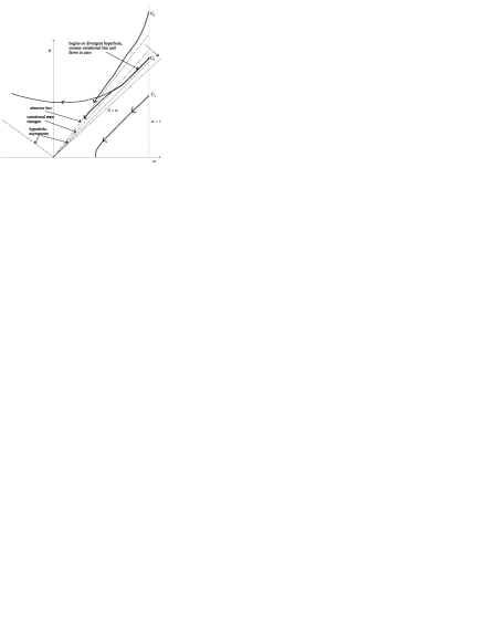
Figure 3.11: Phase space diagram for finite $N$ in the first scheme, with tracking of the ground state expectation value.

familiar from the original Pirner and Friman scheme. The variational line is the point at which the variational state changes from the constant $\left|\Psi\right>=\left|-j\right>$ everywhere in the first phase into a continuously varying paired state in the second phase, as in the variational result (3.127). Above this line the new equations on the right hand side of Eqs. (3.129) come into play. Although there is no simple first integral for these equations, as there are for the first phase, it is not difficult to show that the attractor line serves as an attractor for the flow, along which the flow will remain. Thus we have removed the original divergent results of Pirner and Friman, since now in the second phase all curves must eventually end at the origin. The only complication is that, since $\beta_{\mbox{\scriptsize asymptotes}}<\beta_{\mbox{\scriptsize variational}}$ for finite $N$, there is a small region of $\beta_{0}$ close to $1$ in which the flow initially starts out on the divergent branch of the hyperbola, only to flow to zero when the variational state begins to change (this shall be termed the initial hyperbola effect). All three lines tend toward $\beta=\alpha$ for large $N$.

In this way tracking the evolution of the ground state during the flow has led to sensible results for all $\beta_{0}$. The ground state energy $E^{1}_{N}(\beta_{0})$ and the gap $\Delta^{1}_{N}(\beta_{0})$ reproduce Pirner and Friman’s results (3.39) and (3.41) in the first phase, as the variational state is not sensitive to changes there. $E_{0}$ must be calculated numerically in the second phase, while $\Delta$ is identically zero there (see Fig. 3.12).

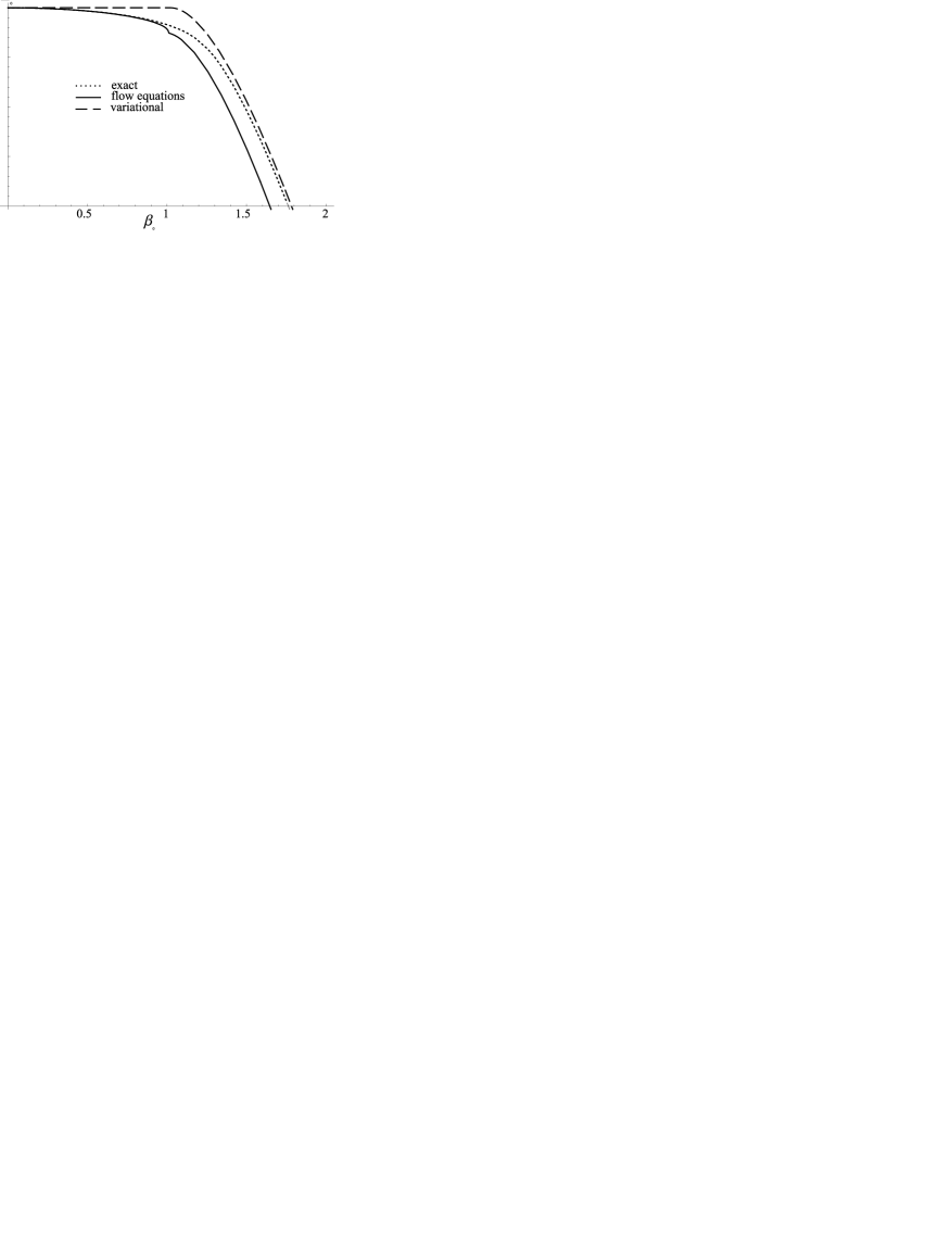
(a)

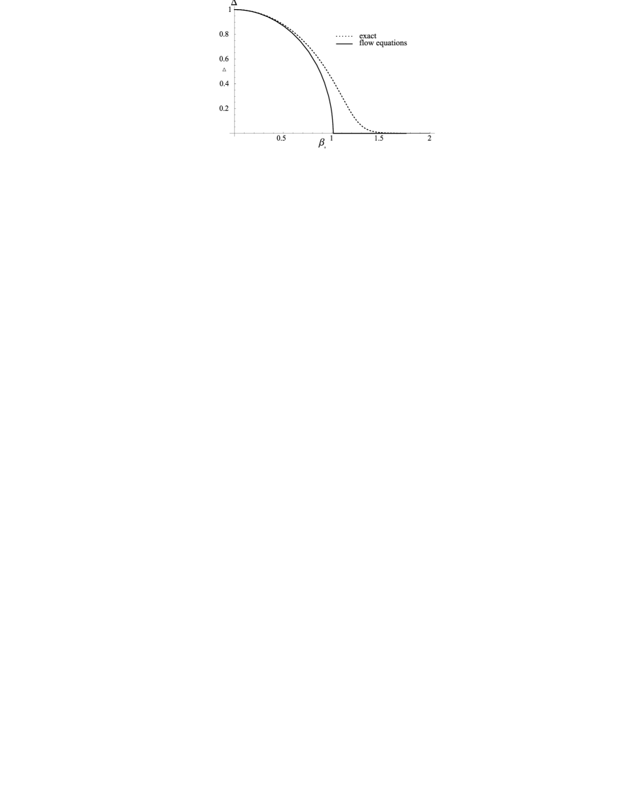
(b)

Figure 3.12: (a) Ground state energy $E_{0}$ and (b) gap $\Delta$ for $N=50$ particles. The squiggle which occurs for finite $N$ is due to initial hyperbola effect.

3.6.2 Second scheme

The same game can now be played for the second scheme where we include a $J_{z}^{3}$ term in the flow with coefficient $\gamma$, as we did before in Eq. (3.43). The variational state must be recalculated since the form of the Hamiltonian has changed. The result from Appendix LABEL:AVarCalc shows that there is again a line

$$\beta_{\mbox{\scriptsize variational}}^{(2)}=g(j)\alpha+f(j)$$ (3.133)

across which the variational state begins to change,

$$\left<z_{v}(\alpha,\beta)\right|J_{z}\left|z_{v}(\alpha,\beta)\right>=\left\{\begin{array}[]{c@{\quad\quad}l}-j&\beta\leq\beta_{\mbox{\scriptsize variational}}^{(2)}\\ -j\left(1-2\frac{h(\alpha,\beta,j)^{2}}{1+h(\alpha,\beta,j)^{2}}\right)&\beta>\beta_{\mbox{\scriptsize variational}}^{(2)}\end{array}\right.,$$ (3.134)

with $f,g,h$ having a rather complicated $j$-dependency:

$$f(j) = \frac{2j(6j^{2}-6j+2)}{4j^{3}+2j^{2}-4j+1}=3+{\cal O}(1/j)$$ (3.135)

$$g(j) = \frac{-2j(4j^{2}-8j+3)}{4j^{3}+2j^{2}-4j+1}=-2+{\cal O}(1/j)$$ (3.136)

$$h(\alpha,\beta,j) = \sqrt{\frac{3-4\alpha+\sqrt{12(\alpha-1)\alpha+\beta^{2}}}{3-2\alpha+\beta}}+{\cal O}(1/j).$$ (3.137)

Before we use 3.134, we shall first eliminate the $J_{z}^{3}$ coefficient $\gamma$ from the flow equations using Eq. (3.52) so as to reduce our variables only to $\alpha$ and $\beta$. The flow equations (3.49), (3.50) and (3.51) become

$$\dot{\alpha} = \beta^{2}\left(\frac{2j(j+1)-1}{j^{2}}\right)$$ (3.138)

$$\dot{\beta} = -4\beta\left(\alpha-\frac{6(\alpha-1)\left<J_{z}\right>^{2}}{2j(j+1)-1}\right).$$ (3.139)

Now we use the variational result (3.134) to obtain the

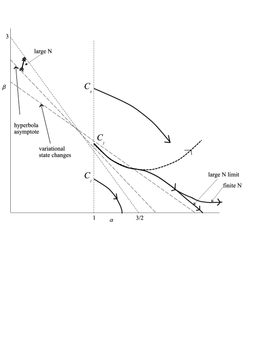
Figure 3.13: Phase space diagram for finite $N$ in the second scheme, with tracking of the ground state expectation value.

flow equations on both sides of the $\beta_{\mbox{\scriptsize variational}}$ line. The equations shall only be displayed in the large $N$ limit for simplicity; the reader is welcome to inspect the full $j$-dependent expression for $h(\alpha,\beta,j)$ (LABEL:Bigh) if desired!

$$\begin{array}[]{rcl@{\quad\quad}rcl}\lx@intercol\hfil\beta\leq\beta_{\mbox{\scriptsize variational}}\hfil\lx@intercol&\lx@intercol\hfil\beta>\beta_{\mbox{\scriptsize variational}}\hfil\lx@intercol\\ \hline\cr\dot{\alpha}&=&2\beta^{2}&\dot{\alpha}&=&2\beta^{2}\\ \dot{\beta}&=&-4\left(\alpha\beta+3\beta(1-\alpha)\right)&\dot{\beta}&=&-4\left(\alpha\beta+3\beta(1-\alpha)\left(\frac{\beta+2\alpha-\sqrt{12\alpha(\alpha-1)+\beta^{2}}}{\beta-6\alpha+6+\sqrt{12\alpha(\alpha-1)+\beta^{2}}}\right)^{2}\right)\end{array}.$$ (3.140)

The structure of the phase space is shown in Fig. 3.13. The first phase equations (the left hand side of (3.140)) are identical to those obtained previously in Eqs. (3.49)-(3.51). For $\beta_{0}<\beta_{\mbox{\scriptsize asymptotes}}^{(2)}$ as in ${\cal C}_{1}$ the flow begins at $(1,\beta_{0})$ and flows to the right along the lower branch of the hyperbola with asymptote

$$\beta_{\mbox{\scriptsize asymptotes}}^{(2)}=\frac{12j^{4}}{(2j(j+1)-1)^{2}}.$$ (3.141)

The off-diagonal $\beta$ term decreases and $\cal H$ is diagonalized as $\ell\rightarrow\infty$. For $\beta_{\mbox{\scriptsize asymptotes}}^{(2)}<\beta_{0}<\beta_{\mbox{\scriptsize variational}}^{(2)}$, the flow begins to flow to infinity along the upper divergent hyperbola. Soon it crosses the line $\beta_{\mbox{\scriptsize variational}}^{(2)}$ and starts to obey the flow equations on the RHS of (3.140). At this point the flow changes direction, and begins to flow toward diagonal form (i.e. towards the $\alpha$ axis).

At this point it is crucial to investigate the behaviour of the RHS of the $\dot{\beta}$ equation in (3.140), so as to determine if $\beta$ will ultimately decrease to zero (thus diagonalizing ${\cal H}$), or if $\beta$ will somehow diverge away as before. The answer to this question lies in Fig. 3.14, which plots the sign of $\dot{\beta}$ in the phase space. For finite $N$ there is a small sliver just above the $\alpha$ axis in which $\dot{\beta}$ becomes positive. Thus, for finite $N$, the matrix approaches diagonal form very closely, only

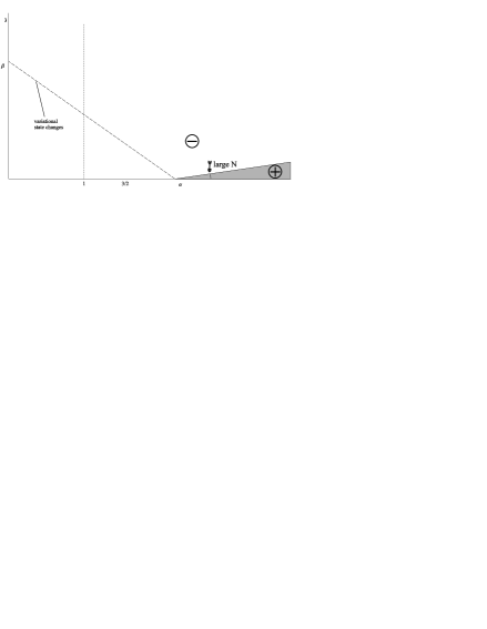
Figure 3.14: The sign of the full $j$ dependent $\dot{\beta}$.

to diverge away at the last moment, as shown in ${\cal C}_{2}$. The positive region becomes ever thinner as $N$ increases, so that in the large $N$ limit ${\cal H}$ does indeed flow to diagonal form, as in ${\cal C}_{3}$. In this case we produce the same results for $E_{0}$ and $\Delta$ as in Fig. 3.12.

The task remains to explain why our method, of tracking the ground state during the flow and adjusting the linearization accordingly, has come close but failed to diagonalize $\cal H$ in the second phase. The answer probably lies in the linearization step (3.47). Recall that the order in which linearization or commutation is applied makes a difference:

$$[\cdot,\cdot]\circ\mbox{linearize} \rightarrow -6\left<J_{z}\right>^{2}(J_{+}^{2}+J_{-}^{2})$$ (3.142)

$${}\mbox{linearize}\circ[\cdot,\cdot] \rightarrow \left(12(1-\left<J_{z}\right>)J_{z}+6\left<J_{z}\right>^{2}-8\right)J_{+}^{2}+conj.$$ (3.143)

To obtain a measure of which order is more accurate, we define

$$A_{\mbox{\scriptsize first}}(\alpha) = ||\,[J_{+}^{2}-J_{-}^{2},J_{z}^{3}]\Psi-\left(-6\left<J_{z}\right>^{2}(J_{+}^{2}+J_{-}^{2})\right)\Psi||$$ (3.144)

$$A_{\mbox{\scriptsize second}}(\alpha) = ||\,[J_{+}^{2}-J_{-}^{2},J_{z}^{3}]\Psi-\left(\left(12(1-\left<J_{z}\right>)J_{z}+6\left<J_{z}\right>^{2}-8\right)J_{+}^{2}+conj.\right)\Psi||,$$ (3.145)

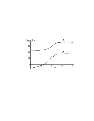
Figure 3.15: The error involved in linearizing first ($A_{\mbox{\scriptsize first}}$) or linearizing second ($A_{\mbox{\scriptsize second}}$). $N=50$ particles.

where the subscripts refer to whether linearization is applied first or second with respect to commutation. $\Psi$ is the exact ground state of the Hamiltonian. The $\alpha$ dependency enters because we intend to evaluate these functions along the line $(\beta=1,\alpha=0\ldots 2)$, which passes through both regions of phase space. Along this line $\Psi$ will change, and so too will $\langle J_{z}\rangle$ since it is a function of $\alpha$ and $\beta$ from Eq. (3.134). The idea is simply to measure which method comes closest to approximating the action of $[J_{+}^{2}-J_{-}^{2},J_{z}^{3}]$ on the ground state. The results are plotted on a logarithmic scale in Fig. 3.15. It is clear that linearizing second is orders of magnitude more accurate than linearizing first. This was to be expected, since it is theoretically the sounder scheme. Unfortunately it is not easy to implement, as it necessarily involves adjoining new operators to the flow ($J_{z}J_{+}^{2}+J_{-}^{2}J_{z}$), which themselves produce new operators, and so on. Fig. 3.15 also clearly shows how the linearization procedure is poorer in the second phase ($\beta_{0}>1$), where the structure of the ground state is more complex.

In conclusion we see that the algebraic structure of the Hamiltonian has made it difficult to consistently follow a linearization procedure, when a $J_{z}^{3}$ term is added to the flow. One is forced to linearize in an ad hoc fashion, which introduces finite $N$ errors that ultimately prevent the Hamiltonian from being diagonalized in the second phase.

3.7 Self-consistent linearization

The drawback of the previous scheme is that a variational calculation was necessary as an outside addition to the process. It would be desirable to eliminate this step by calculating $\langle J_{z}\rangle(\ell)$ in a self-consistent manner. This is indeed possible, in a scheme that has recently been outlined by one of the supervisors of this work [46]. To do this we note that it cannot have an explicit dependence on $\ell$, but rather can only depend on $\ell$ implicitly though its dependence on the $\ell$-dependent parameters $\alpha(\ell)$ and $\beta(\ell)$. This in turn is because the dynamical ground state $\left|G(\alpha(\ell)\right>$ cannot have an explicit dependence on $\ell$ since the Hamiltonian $H(\alpha(\ell),\beta(\ell),\delta(\ell))$ does not have such a dependence. Furthermore, we note that $\langle J_{z}\rangle(\ell)$ can only be a function of the dimensionless coupling constant $x(\ell)\equiv\beta(\ell)/\alpha(\ell)$, since the constant $\delta$ and rescaling by $1/\alpha$ do not affect expectation values. This implies that we can write

$$\langle J_{z}\rangle(\ell)\equiv\langle G,\ell|J_{z}|G,\ell\rangle\equiv f(\beta(\ell)/\alpha(\ell)).$$ (3.146)

Now we differentiate $f(\beta(\ell)/\alpha(\ell))$ with respect to $\ell$, and use the flow equations (3.33)-(3.35) to obtain

$$\left[\frac{\beta^{3}}{j^{2}\alpha^{2}}\left(6f^{2}(\beta/\alpha)-2j(j+1)+1\right)-4\beta\right]f^{\prime}(\beta/\alpha) = -\langle G,\ell|[\eta,J_{z}]|G,\ell\rangle$$ (3.147)

$$= 4(E_{g}-\alpha f(\beta/\alpha)-j\delta)$$ (3.148)

where the second line follows from substituting the form of the generator $\eta$ from 3.45 and the parameterization of the original Hamiltonian 3.6. Now we differentiate this result again with respect to $\ell$ and use the flow equations (3.33)-(3.35) again. The remarkable result is that we now obtain a closed differential equation for $f(x)$, where $x=\beta/\alpha$ is the dimensionless coupling constant,

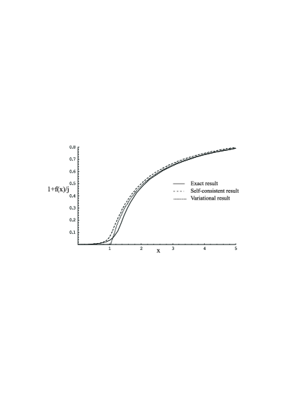
Figure 3.16: Order parameter $1+f(x)/j$ as a function of the dimensionless coupling constant $x$, for $N=30$ particles. The legend distinguishes the exact result, variational result and self-consistent result.

$$\left[\frac{x^{2}}{j^{2}}\left(6f^{2}(x)-2j(j+1)+1\right)-4\right]^{2}f^{\prime\prime}(x)+(\frac{2x^{3}}{j^{4}}-\frac{8x}{j^{2}})\left(6f^{2}(x)-2j(j+1)+1\right)^{2}f^{\prime}(x)$$

$$+\frac{12x^{4}}{j^{4}}\left(6f^{2}(x)-2j(j+1)+1\right)f^{\prime 2}(x)f(x)-\frac{48x^{2}}{j^{2}}f^{\prime 2}(x)f(x)\hskip 85.35826pt$$

$$-\frac{4}{j^{2}}\left(6f^{2}(x)-2j(j+1)+1\right)f(x)+\frac{16}{j^{2}}f^{3}(x)=0.\hskip 113.81102pt$$ (3.149)

This is a non-linear differential equation that uniquely determines the function $f(x)$ once boundary conditions have been specified. It is useful to define $1+f(x)/j$ as an order parameter, since in the thermodynamic limit this quantity vanishes everywhere for $x<1$ and is equal to unity for $x>1$. This last statement follows from the fact that the expectation value $\langle J_{z}\rangle$ scales linearly with $j$ in the weakly coupled system($x<1$) but does not scale with $j$ in the strongly coupled system($x>1$). In principle Eq. (3.149) contains all information on the phase structure of the system. All that remains is to determine the boundary conditions on $f(x)$. These are easily derived by noting that at $x=0$ the Hamiltonian is ${\cal H}=J_{z}$ so that $f(0)=-j$. Furthermore, since $f(-x)=f(x)$, one easily sees that $f(x)$ attains its minimum value at $x=0$. Thus we have the boundary conditions

$$f(0)=-j,\quad f^{\prime}(0)=0$$ (3.150)

In Fig. 3.16 the order parameter $1+f(x)/j$ is plotted as a function of $x$ for $j=15$. The exact result(from numerical diagonalization) and the variational result from (3.128) is also shown for comparison. We note excellent agreement, even in the transitional regions where the fluctuations are large. In the two different phases where the fluctuations are expected to be small, the self-consistent result indeed converges to the exact result. The variational result is a marginally better approximation in the second phase, but is noticeably poorer in the transitional region.

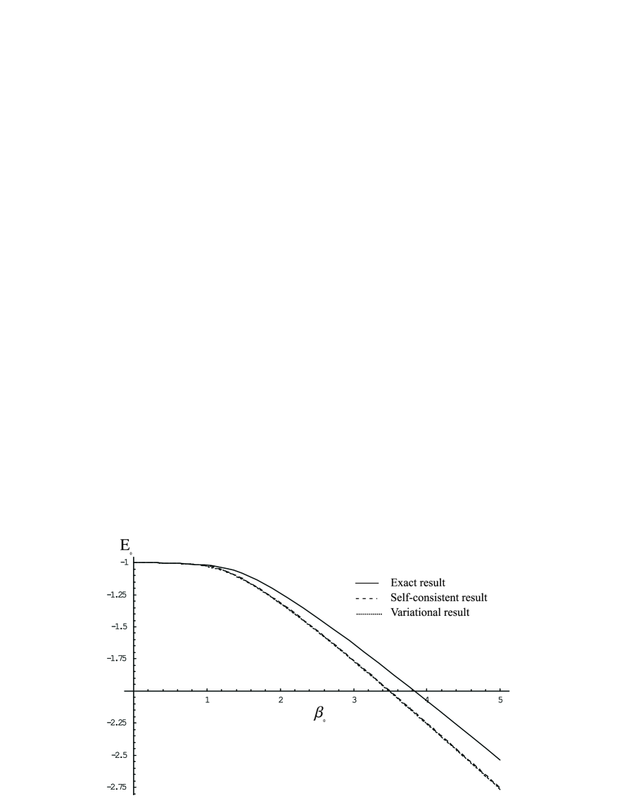
(a)

(b)

Figure 3.17: (a) Ground state energy $E_{0}$ and (b) gap $\Delta$ for $N=30$ particles. The legend distinguishes the exact result, the flow equations result using the variational calculation, and the flow equations result using the self-consistent calculation.

Once $f(x)=\langle J_{z}\rangle$ has been numerically computed from (3.149), the flow equations (3.33)-(3.35) can be integrated, as was done previously in Section 3.6 using the variational calculation of $\langle J_{z}\rangle$. This allows us to compare the results for the ground state energy and the gap, which are presented in Fig. 3.17(a) and Fig. 3.17 (b). The result for the ground state is virtually indistinguishable from that obtained previously when a variational calculation was employed. This is a remarkable success of the method, since it used no external information and had to generate “its own” $\langle J_{z}\rangle$. However the result from the gap, while faring better than that obtained from a variational calculation in the first phase, fares markedly poorer in the second phase. This result shows how the small difference in $\langle J_{z}\rangle$ present between the two approaches in Fig. 3.16 can create a notable difference after the flow equations have been integrated. Both the self-consistent and variational calculations approach the exact result in the limit of large $N$.

Clearly the success of the method can be generalized to many other systems. The central idea is that the flow equations are closed by linearizing around ground state expectation values. These expectation values are always only implicitly dependent on $\ell$, and can only be an explicit function of one less than the number of parameters in the Hamiltonian, since they are invariant under multiplication of the Hamiltonian by a constant factor. This means that differentiation of these functions together with the use of the flow equations should yield a closed differential equation for the order parameter(in this case the expectation value), in a self-consistent manner. Integration of this equation then provides one with accurate knowledge of the order parameter and ground state energy, without ever diagonalizing the Hamiltonian or performing an auxiliary calculation.

3.8 Other flow equations approaches to the Lipkin model

Besides the method of tracking the ground state during the flow, we have also investigated other approaches. Although they did not lead to concrete results, they are listed here since all of them are new methods of dealing with the flow equations that haven’t been attempted before.

3.8.1 Operator differential equations

Instead of parameterizing the Hamiltonian during the flow with scalar coefficients, we might try to track the flow with operator valued coefficients. To be precise, we will write the Hamiltonian during the flow as

$${\cal H}(\ell)=f(J_{z},\ell)J_{z}+g(J_{z},\ell)J_{+}^{2}+J_{-}^{2}g(J_{z},\ell).$$ (3.151)

The functions $f(J_{z},\ell)$ and $g(J_{z},\ell)$ are operator valued and have initial conditions

$$f(J_{z},0)=J_{z},\quad g(J_{z},0)=\beta_{0}/4j.$$ (3.152)

Evaluating the double bracket yields

$$[[J_{z},{\cal H}],{\cal H}]=4\left[g^{2}(J_{z})B(J_{z})+A(J_{z})A(J_{z}+1)(g^{2}(J_{z})-g^{2}(J_{z}+2))\right]$$ (3.153)

$$-\left[2g(J_{z})(f(J_{z})-f(J_{z}-2))\right]J_{+}^{2}-J_{-}^{2}\left[2g(J_{z})(f(J_{z})-f(J_{z}-2))\right],$$ (3.154)

where $B(J_{z})=-8J_{z}^{3}+(8j(j+1)-4)J_{z}$ and $A(J_{z})=-J_{z}^{2}-J_{z}+j(j+1)$. We have thus obtained a closed set of differential equations for $f$ and $g$:

$$\frac{\partial f(J_{z},\ell)}{\partial\ell} = 4\left[g^{2}(J_{z})B(J_{z})+A(J_{z})A(J_{z}+1)(g^{2}(J_{z})-g^{2}(J_{z}+2))\right]$$ (3.155)

$$\frac{\partial f(J_{z},\ell)}{\partial\ell} = -2g(J_{z})(f(J_{z})-f(J_{z}-2)).$$ (3.156)

The fact that the equations are closed was to be expected since Eq. (3.151) is the most general band-diagonal matrix, and we have already shown that the Hamiltonian remains band-diagonal during the flow. It is important to compare Eqs. (3.155) and (3.156) with the direct equations for the diagonal elements $\varepsilon_{n}$ and off-diagonal elements $\theta_{n}$, as in Mielke’s treatment(Eqs. (3.77) and (3.78)),

$$\frac{d\varepsilon_{n}}{d\ell} = 4(\theta_{n+2}^{2}-\theta_{n}^{2})$$ (3.157)

$$\frac{d\theta_{n}}{d\ell} = -2\theta_{n}(\varepsilon_{n}-\varepsilon_{n-2}).$$ (3.158)

If we write $f_{m}=\langle m|f(J_{z})|m\rangle$ and $g_{m}=\langle m|g(J_{z})|m\rangle$, then the two are related by a change of variables

$$\varepsilon_{m}=mf_{m},\quad\theta_{m}=\sqrt{(j-m+2)(j-m+1)(j+m)(j+m-1)}g_{m}.$$ (3.159)

What we have gained, though, in writing the flow equations in the variables $f_{m}$ and $g_{m}$, is that the initial conditions are much simpler. This is illustrated in Fig. 3.18, for the case of the off-diagonal entries.

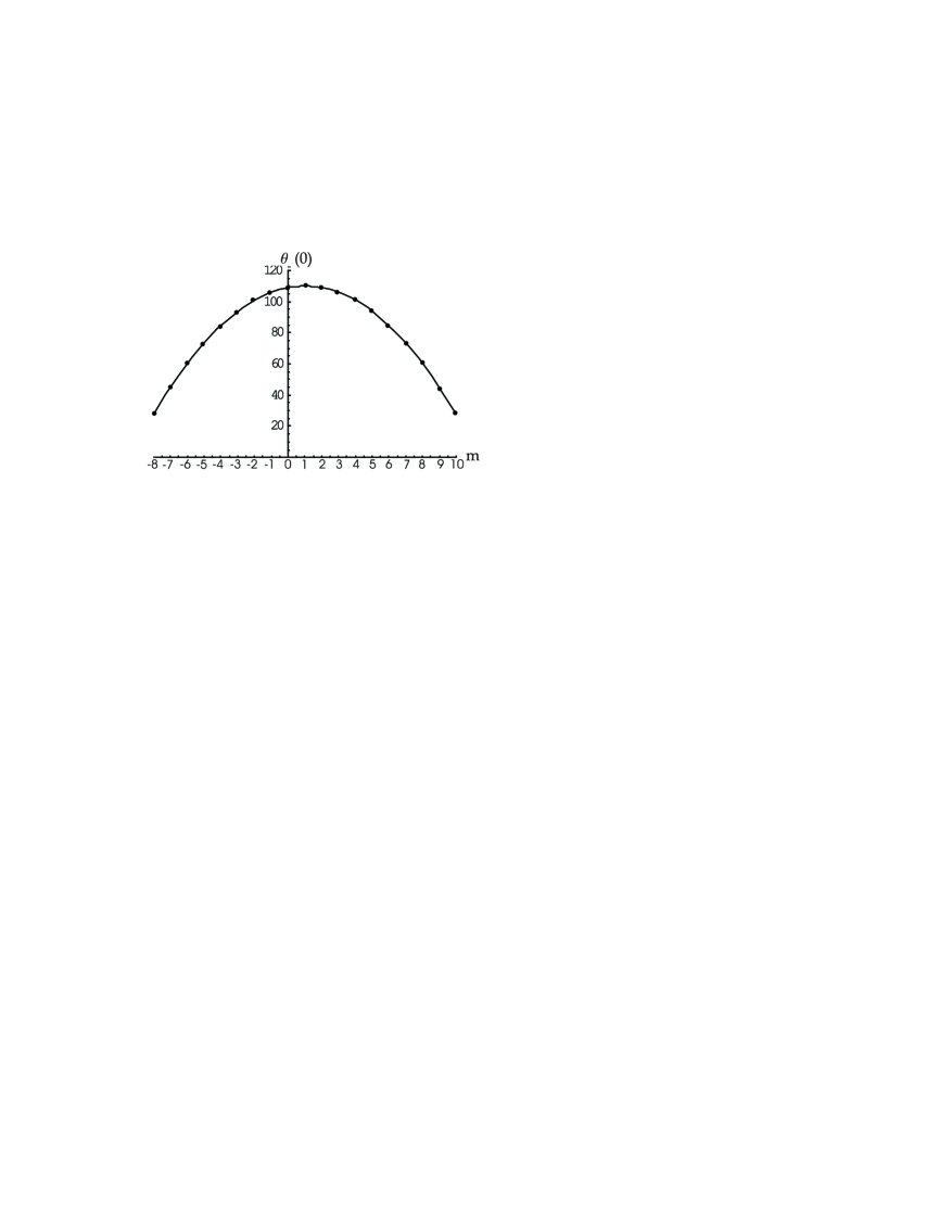
(a)

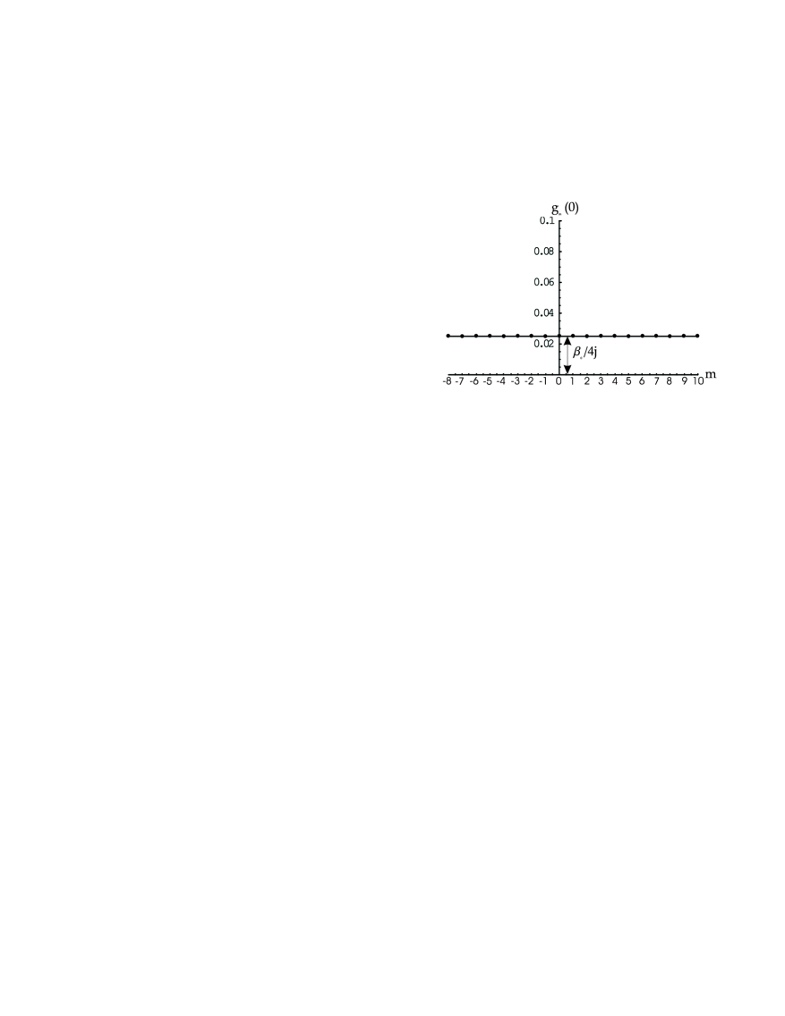
(b)

Figure 3.18: Comparison between initial conditions, contrasting the curve (a) $\theta_{m}(0)$ with (b) the horizontal line $g_{m}(0)$.

Nevertheless, the new system of equations (3.155)-(3.156), was still unable to cope with the second phase($\beta_{0}>1$) in a powerful way, after using the same type of nonperturbative approximation that Mielke used in Section 3.4. The reason is that in the second phase, though $g_{m}$ begins as a straight horizontal line at $\ell=0$, the exact solution shows that it rapidly develops two sharp bumps on each end, which invalidate the approximation made. This can be traced back to the boundary effects present in Fig. 3.9.

In a more general context, by writing the Hamiltonian using $\ell$ dependent operators instead of scalars it may be possible to find a closed operator form of the Hamiltonian during the flow. This immediately eliminates redundant parameters and may give a deeper insight into the problem.

3.8.2 Moment preservation

Under the exact unitary flow of the Hamiltonian, all moments will remain invariant:

$$\mbox{Tr}({\cal H}^{i}(\ell))=\mbox{Tr}({\cal H}_{0}).$$ (3.160)

Indeed, this can be regarded as a definition of unitary equivalence. When approximations are made in the flow equations, the invariance of the moments is lost and the traces begin to change. One may attempt to choose the parameters in the Hamiltonian in such a way as to strictly maintain one of the moments during the flow. Out of the myriads of possible schemes that present themselves in this way, we will focus here on the simplest choice. We use the first scheme parametrization of the Hamiltonian,

$${\cal H(\ell)}=\alpha J_{z}+\frac{\beta}{4j}(J_{+}^{2}+J_{-}^{2})+\delta.$$ (3.161)

$\alpha(\ell)$ and $\beta(\ell)$ are taken from the first scheme solution to the flow equations when the ground state is tracked during the flow, as in Eq. (3.129). However, $\delta(\ell)$ is chosen so that the second order moment

$$\mbox{Tr}({\cal H}^{i})=\alpha^{2}\frac{(2j+1)(j+1)j}{3}+\beta^{2}\frac{(2j+3)(2j+1)(2j-1)(j+1)}{60j}+\delta^{2}(2j+1)(j)$$ (3.162)

is preserved. The second order moment is chosen due to its relative simplicity; other orders are obviously also possible. Explicitly, we set

$$\delta=-\frac{\sqrt{20j^{2}(2j+1)(j+1)(1-\alpha^{2})+(4j(1+j)-3)(\beta_{0}^{2}+\beta^{2})}}{2j\sqrt{15(2j+1)}}.$$ (3.163)

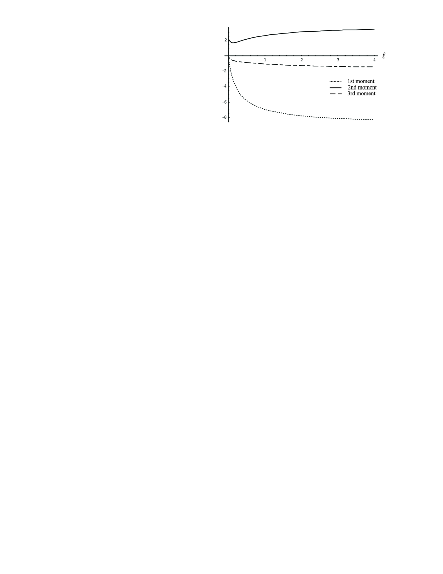
(a)

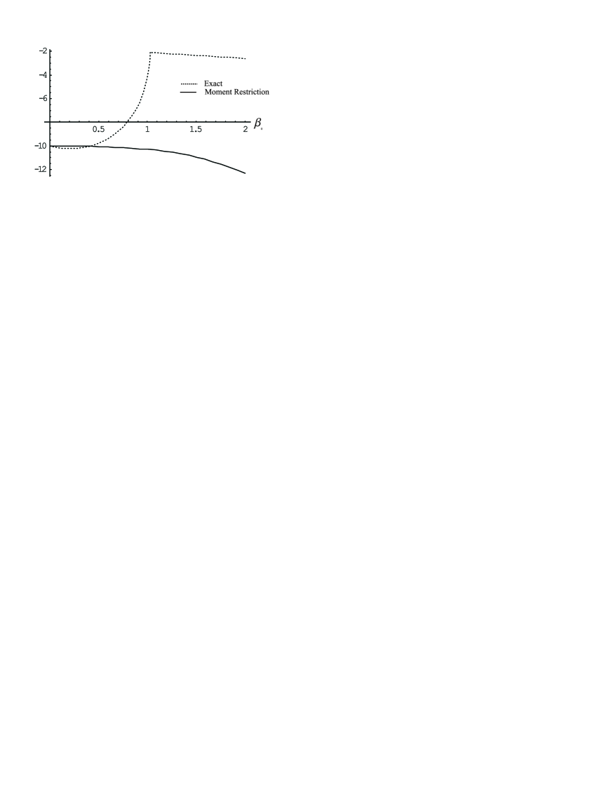
(b)

Figure 3.19: (a) Flow of first three moments, for $\beta_{0}=1$. Moments are normalized by $1/N$, $1/N^{2}$ and $1/N^{3}$. (b) Effect of utilizing the moment preservation equation (3.163).

The results are shown in Fig. 3.19. For the reader to get an idea of how the various moments change with $\ell$, Fig. 3.19(a) plots the flow of the first three moments, normalized appropriately. Fig. 3.19(b) plots the result, using the moment preservation equation (3.163) and the known first scheme solution for $\alpha(\infty)$ from Section 3.6, for the ground state $E_{0}$. It is not surprising to see that preserving the second moment in a parametrization like Eq. (3.161) is a very poor approximation if one is interested in the ground state properties. The reason is that preserving the moments is attempting to find the closest fit to the whole exact Hamiltonian during the flow, whereas we are only interested in the ground state. More sophisticated methods, involving different parametrizations, and different definitions of the trace operation so as to zero in on the lowest lying states, produce slightly better results, although the complexity involved is also significantly increased.

3.8.3 Generator flow

So far we have viewed the flow as taking place either in ${\cal C}({\cal H}_{0})=\{H\;:\;H\mbox{ is unitarily equivalent to }{\cal H}_{0}\}$, or in $SU(N)$. We may go a step further and consider the flow as taking place in the Lie Algebra of $SU(N)$, namely su$(N)$(See Fig. 3.20).

In other words, if we write the unitary transformations in the exponential form

$$U(\theta_{i})=e^{\sum_{i}\theta_{i}K_{i}},$$ (3.164)

then we consider the flow as taking place in the generator space $K_{i}$. The hope is to remove that part of the non-linearity of the flow equations which is due to the exponential. For instance, consider a $2\times 2$ matrix, with real coefficients:

$$H_{0}=\left(\begin{array}[]{ccc}1&t\\ t&2\\ \end{array}\right).$$ (3.165)

This may be viewed as a reduced Lipkin model with $J_{z}=\mbox{Diag}(1,2)$. Let $Q$ be the real orthogonal matrix that transforms the Hamiltonian. We know from Section 1.3.3 that $\dot{Q}=-Q\eta$, where $\eta=[J_{z},Q^{T}H_{0}Q]$. Thus if we write

$$Q(\theta)=e^{\theta K}\leftrightarrow\left(\begin{array}[]{cc}\cos\theta&\sin\theta\\ -\sin\theta&\cos\theta\end{array}\right)=\mbox{Exp}\left(\begin{array}[]{cc}0&1\\ -1&0\end{array}\right),$$ (3.166)

then the differential equation for $\dot{\theta}$ is

$$\dot{\theta} = t\cos(2\theta)-\frac{1}{2}\sin(2\theta)$$ (3.167)

$$\theta(0) = 0.$$ (3.168)

If we were hoping for a simpler differential equation, then we have failed dismally, as this equation is more complex than the direct Hamiltonian matrix elements version

$$\dot{\varepsilon_{1}}=-2v^{2},\quad\dot{\varepsilon_{2}} = 2v^{2},\quad\dot{v}=-v(\varepsilon_{2}-\varepsilon_{1})$$ (3.169)

$$\varepsilon_{1}(0)=1,\quad\varepsilon_{2}(0) = 2,\quad v(0)=t,$$ (3.170)

where $\varepsilon_{i}=H_{ii}$ and $v=H_{12}$. But we have gained in two areas. Firstly, the flow has been reduced from three variables to one. For a general real Hamiltonian of size $N$, there would be $\frac{1}{2}N(N+1)$ equations in the Hamiltonian matrix elements, and $\frac{1}{2}N(N-1)$ equations in $so(N)$. Secondly, the boundary condition has been shifted into the equation for $\dot{\theta}$. This may be useful if one is interested in the onset of a phase change, as investigation of the instability of the equations would give direct information on the parameter values involved at the transition point.

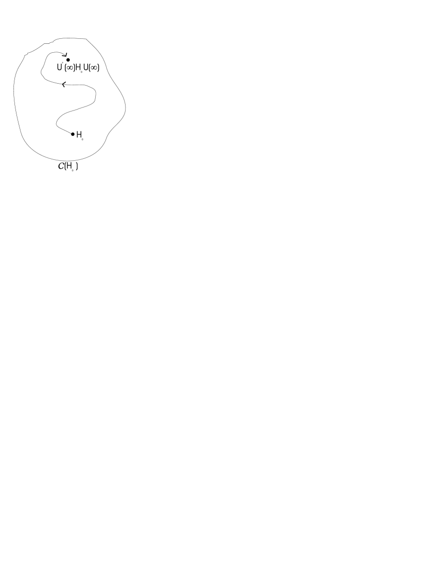
(a)

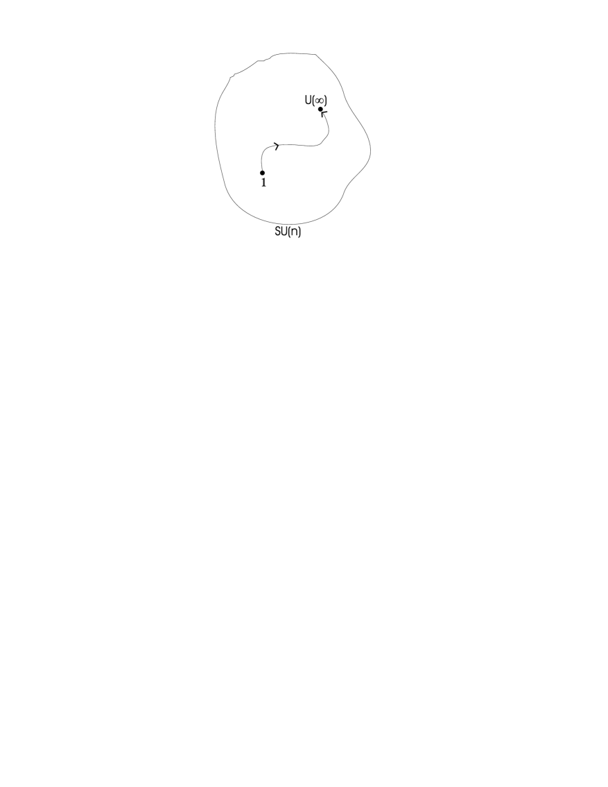
(b)

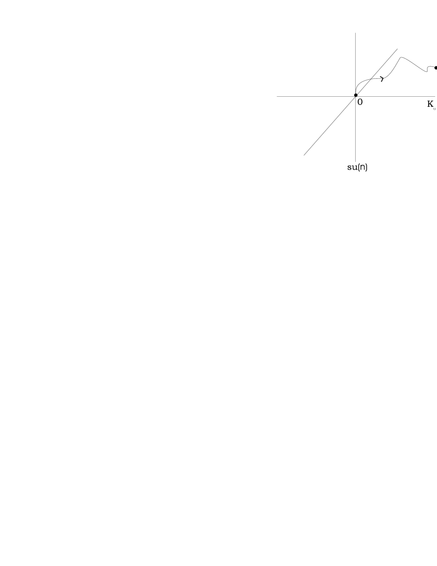
(c)

Figure 3.20: The flow in (a) ${\cal C}({\cal H}_{0})$, (b) $SU(N)$ and (c) $su(N)$

In addition, it might be possible by a clever choice of the generators $K_{i}$ to effectively decouple the equations for the $\theta_{i}$, and hence “straighten the flow”. We know this is always mathematically possible from differential geometry (eg. see Ref. [47]). In the Lipkin model, one might use

$$K_{ij}=\frac{J_{z}^{j-1}J_{+}^{i}-J_{-}^{i}J_{z}^{j-1}}{\left(N/2\right)^{i+j-1}}\qquad i=1\ldots N,\,j=1\ldots N+1-i$$ (3.171)

as a basis for the generator space. Unfortunately, again, this choice works well for small $\beta_{0}$ where the unitary transformation is approximately of the form

$$U=e^{\theta_{11}K_{11}}=e^{\theta_{11}(J_{+}^{2}-J_{-}^{2})}.$$ (3.172)

Indeed, this is familiar from the first scheme in Section 3.6, where $\eta=[J_{z},{\cal H}]\propto J_{+}^{2}-J_{-}^{2}$. However for larger $\beta_{0}$ near the phase change, other $\theta_{ij}$ become important and the approximation is not so good anymore.

3.9 Discussion

We have presented various different methods of dealing with the Lipkin model by flow equations. The first replaced newly generated operators by linearizing them around the zero interaction ground state. The second considered the matrix elements themselves and provided a non-perturbative solution correct for large $N$. The third used the Holstein-Primakoff mapping to systematically solve the flow equations order for order in $1/N$. The fourth method improved on the first by employing a variational calculation to track the ground state, and hence the expectation value relevant to the linearization, during the flow. The specific choice of a variational state to approximate the ground state is not crucial to the method, and any approximate input as to the nature of the ground state during the flow wold have produced similar results. The fifth method dispensed with the outside input necessary in the previous technique by utilizing a self-consistent calculation of the expectation value. This resulted in very similar results to the previous method for the ground state energy, as well as providing a simple and exciting new way to calculate an order parameter such as the expectation value.

Only the last two mentioned methods were able to deal with the second phase in a meaningful way, since the flow equations were dynamically altered there due to a changing expectation value. The reason the second phase has proved more difficult to analyze is clear from Figs. 3.5-3.6. The flow is highly nonlinear in this region and the direction of the flow, as specified by the generator $\eta$, changes appreciably as it evolves.

We have also outlined three other possible methods of dealing with the operator flow. Some ideas here might be valuable in a different context.

Chapter 4 Flow equations and renormalization

In the early twenties and thirties a gloomy problem hovered over relativistic quantum field theory. Calculation of properties of even the simplest systems such as the energy of an electron in an atom yielded divergent results for anything but the lowest orders in perturbation theory. Hans Bethe’s seminal paper in 1947, which calculated the Lamb shift between the $2s$ and $2p$ levels in a hydrogen atom, was the first to lead to a finite, accurate result. Renormalization - in its modern perturbative sense - was born. Initially some of the procedures seemed ad hoc and specific to the model under consideration, but modern developments have unified the theory with the language of condensed matter and many body physics. In this chapter we discuss renormalization in a Hamiltonian framework. By the term ‘renormalization’ we mean that the parameters present in the initial bare Hamiltonian will be altered so as to provide a new, effective theory which is equivalent to the old one, but more accessible to study. Two of the pioneers of the modern theory of renormalization, Stan Glazek and Kenneth Wilson, have recently made significant progress in this field by using flow equations to dynamically renormalize the Hamiltonian [4, 5]. In this chapter their method will be introduced and compared with Wegner’s flow equation. This will be followed by two examples of applications of the formalism.

4.1 Glazek and Wilson’s similarity renormalization

Recall that, from a mathematical viewpoint, the primary motivation for Wegner’s flow equation

$$\frac{d{\cal H}}{d\ell}=[[\mbox{Diag}{\cal H},{\cal H}],{\cal H}]$$ (4.1)

was that it defines the steepest path to diagonality. To first order in the coupling, the off-diagonal terms flow as

$$v_{ij}^{(1)}(\ell)=V_{ij}e^{-(E_{i}-E_{j})^{2}\ell},$$ (4.2)

where $E_{i}$ and $V_{ij}$ are the initial diagonal and off-diagonal elements respectively. In this way we see that interaction terms coming from states with large energy differences are decoupled first. However, to second order the matter is not so clear-cut, and the renormalization properties of Wegner’s generator (4.1) are not entirely clear. Although Glazek and Wilson developed their similarity renormalization scheme at the same time as Wegner invented his flow equation, in hindsight it is clear that their scheme follows from imposing stricter renormalization requirements than Wegner’s scheme.

The idea is to construct a continuum of unitarily equivalent Hamiltonians $H_{\lambda}$, which interpolate between the initial Hamiltonian ($\lambda=\Lambda$) and the effective Hamiltonian ($\lambda=\lambda_{0}$). The parameter $\lambda$ has the dimensions of energy and is a measure of the size of the largest energy differences that play a role in $H_{\lambda}$. These statements will be made more precise in what follows.

As usual, we separate $H_{\lambda}$ into its diagonal and interacting (off-diagonal) parts

$$H_{\lambda}=H_{0\lambda}+H_{I\lambda}.$$ (4.3)

The diagonal entries of $H_{0\lambda}$ are denoted by $E_{\lambda}$:

$$\langle i|H_{0\lambda}|i\rangle=E_{i\lambda}.$$ (4.4)

As discussed before in Section 1.1, an arbitrary unitary flow can be described as

$$\frac{dH_{\lambda}}{d\lambda}=[T_{\lambda},H_{\lambda}],$$ (4.5)

where $T_{\lambda}$ is anti-Hermitian. The problem is to choose $T_{\lambda}$ so as to satisfy our requirements. The aim is to eliminate matrix elements $\langle i|H_{\lambda}|j\rangle\equiv H_{\lambda ij}$ whenever these matrix elements would cause large jumps in energy beyond the scale set by $\lambda$, i.e. when $E_{i\lambda}$ is sufficiently separated from $E_{j\lambda}$ and the larger of these is well above $\lambda$ itself. In this way, as $\lambda$ is reduced, the far off-diagonal part of $H_{I\lambda}$ is reduced systematically, in that as $\lambda$ decreases it is mainly terms which jump from much lower energies to energies of order $\lambda$ that are being eliminated - terms with energies of order higher than $\lambda$ have already been eliminated, while terms with energies of order lower than $\lambda$ will be eliminated later.

In order to set up the machinery which will produce the desired effect, we first define an auxiliary function

$$x_{\lambda ij}=\frac{E_{i\lambda}-E_{j\lambda}}{E_{i\lambda}+E_{j\lambda}+\lambda}.$$ (4.6)

This function encodes the ideas discussed in the previous paragraph. Namely, its modulus is close to 1 when one of the

Figure 4.1: The zone function $\bar{u}(x)$

energies is much larger than the other and large in comparison to the cutoff $\lambda$. On the other hand, $x_{\lambda ij}$ is close to 0 when the energies are similar or small in comparison to the cutoff. With this function defined, we may now define zones of the Hamiltonian. Let $\bar{u}(x)$ be a suitable ${\cal C}^{\infty}$ function which satisfies:

$$\bar{u}(x)=\bar{u}(|x|)=\left\{\begin{array}[]{c@{\quad\quad}l}1&|x|\leq x_{1}\\ 0&|x|\geq x_{2}\end{array}\right.,$$ (4.7)

and which drops smoothly from 1 to 0 between $|x|=x_{1}$ and $|x|=x_{2}$ (see Fig. 4.1). $x_{1}$ and $x_{2}$ can be arbitrary, unless they lie outside the energy range of the problem, in which case no flow will take place.

Now we define the zone matrices

$$u_{\lambda ij} \equiv \langle i|u_{\lambda}|j\rangle\equiv\bar{u}(x_{\lambda ij})$$ (4.8)

$$r_{\lambda ij} \equiv \langle i|r_{\lambda}|j\rangle\equiv 1-\bar{u}(x_{\lambda ij}).$$ (4.9)

We shall use these zone matrices to identify zones of an operator $u_{\lambda}[\hat{O}]$ in the following way:

$$\left(u_{\lambda}[\hat{O}]\right)_{ij}=\langle i|u_{\lambda}|j\rangle\langle i|\hat{O}|j\rangle=u_{\lambda ij}\hat{O}_{ij},$$ (4.10)

which is simply a notation for multiplying a matrix by a two index function, and should not be confused with matrix multiplication, although we shall write $u_{\lambda}\hat{O}$ as shorthand for $u_{\lambda}[\hat{O}]$. The regions of $u_{\lambda}\hat{O}$ where $u_{\lambda}=1$, $0<u_{\lambda}<1$ and $u_{\lambda}=0$ will be named zone 1, zone 2 and zone 3 respectively.

We announce our intention to get serious about our renormalization scheme by demanding that

$$H_{\lambda}=u_{\lambda}G_{\lambda}$$ (4.11)

where $G_{\lambda}$ is not yet specified. Let us review the framework we are setting up. Each matrix element $G_{\lambda ij}$ has a corresponding $u_{\lambda ij}$ which multiplies it (see Fig. 4.2).

Given the diagonal elements $E_{i\lambda}$ at a certain value of $\lambda$, and the function $\bar{u}(x)$, the $u_{\lambda ij}$ are determined and may be conveniently arranged on the graph of $\bar{u}(x)$ as in Fig. 4.2(a). The diagonal $u_{\lambda nn}$ always remain at 1 since $x_{\lambda ij}=0$ when $i=j$ from Eq. (4.6). The off-diagonal terms will be arranged in such a way that those involving a large jump in energy are further out than those that involve a smaller jump in energy. Since $x_{\lambda ij}=-x_{\lambda ji}$, the $u_{\lambda ji}$ will be positioned symmetrically opposite the $u_{\lambda ij}$ and have the same value. The idea is that as the flow proceeds (i.e. as $\lambda$ decreases), the $u_{\lambda ij}$ will move away from the line $x=0$, moving into zone 2 where they decrease quickly, and finally into zone 3 where they become zero.

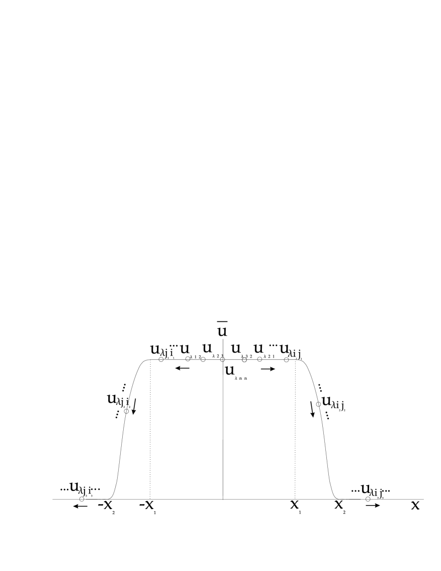
(a)

(b)

Figure 4.2: (a) Behavior of $u_{\lambda ij}$ (b) Zones of $u_{\lambda}$. This diagram is schematic, but is typical for a wide range of Hamiltonians. The arrows indicate the movement of the zones as $\lambda$ decreases.

This may be seen in another way in Fig. 4.2(b), which shows how the zones in the matrix $u_{\lambda}$ will evolve as $\lambda$ decreases. As $\lambda\rightarrow 0$, zone 3 grows at the expense of zone 1 and zone 2 until only the diagonal terms are in zone 1, and all the off-diagonal terms are in zone 3 where they are zero. In this limit $u_{\lambda}$ will be diagonal, and hence $H_{\lambda}$ will be diagonalized from the requirement (4.11).

In terms of $G_{\lambda}$, the unitary flow (4.5) reads

$$\frac{du_{\lambda}}{d\lambda}G_{\lambda}+u_{\lambda}\frac{dG_{\lambda}}{d\lambda}=[T_{\lambda},H_{0\lambda}]+[T_{\lambda},H_{I\lambda}].$$ (4.12)

The initial Hamiltonian $H_{\Lambda}=H_{\lambda\rightarrow\infty}$ is supplied at the beginning of the procedure. In order to obtain equations for $\frac{dG_{\lambda}}{d\lambda}$ and $T_{\lambda}$, let us regard them as unknown, and attempt to solve for them in terms of $u_{\lambda}$, $H_{0\lambda}$, $H_{I\lambda}$ and $G_{\lambda}$. So far there is one equation and two unknowns. In this way the requirement (4.11) has not uniquely specified the flow we are to undertake through unitary space. To produce another equation, we rearrange Eq. (4.12) as

$$[H_{0\lambda},T_{\lambda}]+u_{\lambda}\frac{dG_{\lambda}}{d\lambda}=[T_{\lambda},H_{I\lambda}]-\frac{du_{\lambda}}{d\lambda}G_{\lambda}\equiv Q_{\lambda}.$$ (4.13)

Now we make the rather arbitrary requirement that the manner in which the two terms on the left equal $Q_{\lambda}$ must somehow be in harmony with the zone structure, term for term. We decide that

$$[H_{0\lambda},T_{\lambda}]=r_{\lambda}Q_{\lambda},$$ (4.14)

which means that

$$u_{\lambda}\frac{dG_{\lambda}}{d\lambda}=Q_{\lambda}-r_{\lambda}Q_{\lambda}=u_{\lambda}Q_{\lambda}.$$ (4.15)

We now have two equations for the two unknowns $T_{\lambda}$ and $\frac{dG_{\lambda}}{d\lambda}$ or for $T_{\lambda}$ and $\frac{dH_{\lambda ij}}{d\lambda}$ through the requirement (4.11). These equations must be evaluated for the matrix elements in the three different zones. Specifically, in zone 1($0\leq|x|\leq x_{1}$, $r_{\lambda ij}=0$, $u_{\lambda ij}=1$) we have

$$T_{\lambda ij} = 0$$ (4.16)

$$\frac{dH_{\lambda ij}}{d\lambda} = [T_{\lambda},H_{I\lambda}]_{ij}.$$ (4.17)

In zone 2($x_{1}<|x|<x_{2}$, both $r_{\lambda ij}$ and $u_{\lambda ij}$ between 0 and 1),

$$T_{\lambda ij} = \frac{r_{\lambda ij}}{E_{j\lambda}-E_{i\lambda}}\left([T_{\lambda},H_{I\lambda}]_{ij}-\frac{du_{\lambda ij}}{d\lambda}\frac{H_{\lambda ij}}{u_{\lambda ij}}\right)$$ (4.18)

$$\frac{dH_{\lambda ij}}{d\lambda} = u_{\lambda ij}[T_{\lambda},H_{I\lambda}]_{ij}+r_{\lambda ij}\frac{du_{\lambda ij}}{d\lambda}\frac{H_{\lambda ij}}{u_{\lambda ij}},$$ (4.19)

while in zone 3($|x|>x_{2}$, $r_{\lambda ij}=1$, $u_{\lambda ij}=0$),

$$T_{\lambda ij} = \frac{1}{E_{j\lambda}-E_{i\lambda}}[T_{\lambda},H_{I\lambda}]_{ij}$$ (4.20)

$$\frac{dH_{\lambda ij}}{d\lambda} = H_{\lambda ij}=0.$$ (4.21)

Recall that $u_{\lambda ij}$ is a shorthand for

$$u_{\lambda ij}=\bar{u}\left(x_{\lambda ij}(E_{i\lambda},E_{j\lambda})\right),$$ (4.22)

so that

$$\frac{du_{\lambda ij}}{d\lambda}=\frac{d\bar{u}}{dx}\left(\frac{\partial x}{\partial E_{i\lambda}}\frac{dE_{i\lambda}}{d\lambda}+\frac{\partial x}{\partial E_{j\lambda}}\frac{dE_{j\lambda}}{d\lambda}\right).$$ (4.23)

In this way the renormalization group equations (4.16) - (4.21) may be expressed in the schematic form

$$T_{\lambda ij}=f(T_{\lambda kl},H_{\lambda qr},E_{m\lambda},\frac{dE_{p\lambda}}{d\lambda})$$ (4.24)

$$\frac{dH_{\lambda ij}}{d\lambda}=g(T_{\lambda kl},H_{\lambda qr},E_{m\lambda},\frac{dE_{p\lambda}}{d\lambda}),$$ (4.25)

which shows they are a complicated set of non-linear algebraic and differential equations. Normally the only way to tackle them is through an iterative process or through perturbation theory. The beauty of the equations (4.16) - (4.21) though is that energy denominators only arise for $|x|>x_{1}$ which means, from the expression for the auxiliary function (4.6), that

$$\left|\frac{1}{E_{j\lambda}-E_{i\lambda}}\right|\leq\frac{1}{x_{1}}\frac{1}{E_{i\lambda}+E_{j\lambda}+\lambda},$$ (4.26)

so that a reciprocal of an energy difference cannot be larger than a constant times $\lambda^{-1}$. In this way we have conquered the problem of ordinary perturbation theory where energy denominators can grow arbitrarily small.

For more discussion on the relevance of the similarity renormalization group equations to renormalization problems in quantum field theory (eg. QCD), we refer the reader to the original papers of Glazek and Wilson [4, 5]. Some recent contributions include the analysis of the similarity renormalization group to the Poincar$\acute{e}$ algebra [48], bound-state dynamics of effective fermions [49], and even to theories of gravity [50].

Finally, a comment on the name “Similarity renormalization group”. All the transformations involved are strictly unitary and not just similarity transformations. Of course, since all unitary transformations are also similarity transformations, the designation remains true, albeit imprecise. It appears to be a historical accident from some slightly careless terminology in the original paper in 1993 [5].

4.2 Wegner’s flow equation and the similarity renormalization group

How does Wegner’s flow equation tie in with renormalization, and in particular, the similarity renormalization group equations (4.16)-(4.21)? Both are unitary flows on the initial Hamiltonian, and hence can be written as

$$\frac{d{\cal H}_{\lambda}}{d\lambda}=[F_{\lambda}\{\cal{H}_{\lambda}\},{\cal H}_{\lambda}].$$ (4.27)

In the similarity renormalization approach, $\lambda$ has the dimensions of energy and can be taken to begin at $\lambda=\Lambda\rightarrow\infty$ and asymptotically ends at $\lambda=0$. In Wegner’s flow equation, $\ell$ has the dimensions of 1/$\mbox{energy}^{2}$ and begins at $\ell=0$ and asymptotically ends at $\ell=\infty$. If we set $\ell=1/\lambda^{2}$ then Wegner’s equation

$$\frac{d{\cal H}(\ell)}{d\ell}=[[\mbox{Diag}({\cal H}(\ell)),{\cal H}(\ell)],{\cal H}(\ell)]$$ (4.28)

follows from a specific choice of $F_{\lambda}$, namely

$$F_{\lambda}\{{\cal H}\}=\frac{1}{\lambda^{2}}\frac{d\ell}{d\lambda}[\mbox{Diag}({\cal H}_{\lambda}),{\cal H}_{\lambda}].$$ (4.29)

However, as mentioned in Section 4.1, the renormalization properties of this choice of $F_{\lambda}$ are not entirely clear. In the similarity renormalization group, the equations were derived from first specifying precisely how the Hamiltonian was to change with $\lambda$. The requirements were that states with large energy differences should be treated first, that energy denominators must be bounded with respect to $\lambda$, that as $\lambda$ decreased the far off-diagonal elements become zero (not just very small), and other similar properties resulting from the form of $x_{\lambda ij}$. The price we had to pay for these strict requirements resulted in a complicated set of equations for determining $T_{\lambda}$, and hence $\frac{d{\cal H}}{d\lambda}$.

In contrast, Wegner’s equation is simpler because $T_{\lambda}$ is completely specified, and is chosen so that the Hamiltonian flows in steepest descent fashion either to block-diagonal form or to diagonality. Along the path to block-diagonal form, there is no control over how the off-diagonal elements behave. In particular, the final Hamiltonian could still contain large off-diagonal elements. If the generator is chosen so that the Hamiltonian flows to diagonality, then we know that the off-diagonal matrix elements decrease monotonically, and those with the largest energy differences decrease the fastest. However, there are no other renormalization restrictions (such as zone structure, $\lambda$ dependent bounds on denominators, etc.) on the flow. It should also be noted that although the off-diagonal elements become exponentially small, they never strictly vanish. Perhaps this will be made more clear by remembering that, to first order in the interaction, the off-diagonal elements flow as (from Eq. (1.18))

$$v_{ij}^{(1)}(\ell)=V_{ij}e^{-2(E_{i}-E_{j})^{2}\ell},$$ (4.30)

so that, to first order (and not in general to higher orders), the off-diagonal elements behave as if a uniform gaussian band function $x_{\lambda ij}$ had been chosen in the similarity renormalization group, as opposed to the usual “widening band” structure of the conventional $x_{\lambda ij}$ shown in Fig. 4.2.

4.3 Renormalization in action

Let us continue in the spirit of renormalization via continuous unitary transformations and look at two examples from the literature.

4.3.1 Glazek and Wilson’s discrete 2-d delta function model

The fathers of the similarity renormalization group, Glazek and Wilson, introduced an extremely useful toy model as a testing ground for renormalization type flow equations [51, 52, 53]. The model displays many important characteristics of more complex Hamiltonians since it is asymptotically free, contains a bound state (negative eigenvalue) and has a large range of energy scales.

The model can be considered as a discretized version of the two- dimensional delta function Hamiltonian:

$$H=\frac{\vec{p}^{\;2}}{2m}-g\delta^{2}(\vec{r}).$$ (4.31)

Such Hamiltonians have been studied before. It is known that there is one $s$-wave bound state with a negative eigenvalue. The other eigenstates have positive energies and are $s$-wave scattering states. The model can be discretized by looking at it from a variational principle point of view (see Ref. [52]); we shall not go into the details here. The discretized version is

$$H_{ij}=\delta_{ij}E_{i}-g\sqrt{E_{i}E_{j}},$$ (4.32)

where $E_{i}=b^{i}$ and $b>1$. The parameter $b$ serves roughly as a measure of the severity of the discretization process - as $b\rightarrow 1$, the discretized Hamiltonian approaches the continuous one. For numerical calculations, we shall employ $b=2$. The infinite matrix (4.32) will be made finite by employing an infrared and ultraviolet cutoff. Specifically, the index $i$ ranges from $M$ (a large negative number) to $N$ (a large positive number). Glazek and Wilson chose $M=-21$ and $N=16$, which, if we (with tongue in cheek) call one unit of energy 1 GeV, means that the energy range in the Hamiltonian goes from 0.5 eV to 65 TeV. The coupling constant $g$ is adjusted so that the bound state eigenvalue is precisely -1 GeV, which gives $g=0.06060600631$. Thus the bound state energy scale is three orders of magnitude smaller than the largest energy scale in the problem, and we have in front of us a candidate for renormalization. The model will be renormalized using Wegner’s flow equation which, expressed in terms of the diagonal matrix elements $\varepsilon_{i}$ and the off-diagonal elements $v_{ij}$, are (see Chapter 1)

$$\dot{\varepsilon_{i}} = 2\sum_{k}(\varepsilon_{i}-\varepsilon_{k})v_{ij}^{2}$$ (4.33)

$$\dot{v_{ij}} = -(\varepsilon_{i}-\varepsilon_{j})^{2}v_{ij}+\sum_{k}(\varepsilon_{i}+\varepsilon_{j}-2\varepsilon_{k})v_{ik}v_{kj}.$$ (4.34)

Language familiar to renormalization gurus will be invoked by introducing an effective running coupling constant. Since the initial off-diagonal terms have $H_{ij}=-g\sqrt{E_{i}E_{j}}$, the exact running coupling constant will be defined by

$$\tilde{g}(\ell)=-\frac{H_{M,M+1}(\ell)}{\sqrt{E_{M}E_{M+1}}},$$ (4.35)

where $H(\ell)$ is the exact (obtained numerically) solution to the flow equations. This definition is motivated by the requirement that the coupling constant determines the strength of the interaction at small energies ($E_{M}$ is the smallest energy in the problem), as is standard practice. We can also define an approximate running constant $\tilde{g}_{a}(\ell)$ by allowing the coupling in front of the first order solutions to the flow equation to become $\ell$-dependent:

$$\varepsilon_{i}(\ell) = (1-\tilde{g}_{a}(\ell))E_{i}$$ (4.36)

$$V_{ij}(\ell) = -\tilde{g}_{a}(\ell)\sqrt{E_{i}E_{k}}e^{-(E_{i}-E_{k})^{2}\ell}.$$ (4.37)

If we evaluate $\dot{\varepsilon}_{M}$ by inserting the diagonal entries (4.36) into the flow equation (4.33), and make the approximation $E_{M}-E_{k}\approx-E_{k}$ since $E_{M}$ is very small, we obtain a differential equation for the approximate running coupling constant:

$$\frac{d\tilde{g}}{d\ell}=-\tilde{g}^{2}\frac{d}{d\ell}\sum_{k}e^{-2E_{k}^{2}\ell}.$$ (4.38)

The integration of this equation gives

$$\tilde{g}_{a}(\ell)=\frac{g}{1-g(N+1+0.4+\mbox{ln}(\ell)/\mbox{ln}4)}.$$ (4.39)

The question now is how good an approximation Eqs. (4.36) and (4.37) actually are.

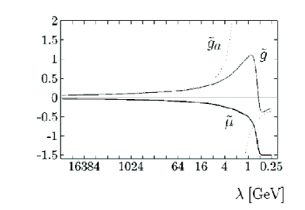
Figure 4.3: The exact and approximate running coupling constants $\tilde{g}$ and $\tilde{g}_{a}$ as functions of the effective Hamiltonian width $\lambda=1/\ell^{2}$. Source Glazek and Wilson, Phys Rev. D 57 3558 (1998)

The answer is provided by Fig. 4.3, which plots the exact and approximate running coupling constants $\tilde{g}$ and $\tilde{g}_{a}$ as functions of the energy width $\lambda=1/\ell^{2}$. In order to compare these graphs with the bound state formation scale (the value of $\lambda$ when the bound state eigenvalue begins to appear on the diagonal), the matrix element

$$\tilde{u}(\ell)=H_{-1,-1}(\ell)-0.5\mbox{ GeV}$$ (4.40)

is also plotted (the bound state eigenvalue appears at $H_{-1,-1}$). $\tilde{u}$ is displaced by 0.5 GeV so as not to obscure the other graphs. The graph shows that the approximate solution blows up in the flow before the effective Hamiltonian width is reduced to the scale where the bound state is formed. However, the exact effect coupling constant does not diverge. This encouraged Glazek and Wilson to expand the solution in terms of the running

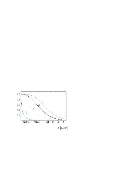
Figure 4.4: The ratio of the bound state eigenvalue of the effective Hamiltonian $H^{(i)}(\ell)$ to the exact result, where $H^{(i)}(\ell)$ is the $i$th perturbative approximation to the exact result in terms of the bare coupling $g$. $\lambda=1/\ell^{2}$. Source Glazek and Wilson, Phys Rev. D 57 3558 (1998)

coupling constant $\tilde{g}(\lambda_{0})$ instead of expanding it in terms of the bare coupling $g$. This point is emphasized in Fig. 4.4, which plots the ratio of the bound state eigenvalue of the effective Hamiltonian $H(\ell)$ to the exact result, where $H(\ell)$ is calculated using the perturbative solution of the flow equations (4.33) and (4.34) to first, second, third and fourth order in the bare coupling $g$. The perturbative solution $H^{(i)}(\ell)$ is diagonalized exactly (numerically) to obtain its bound state eigenvalue. This figure clearly demonstrates that the perturbative expansion in terms of the canonical coupling constant in the initial Hamiltonian is not suitable for applications in the bound state dynamics.

Glazek and Wilson went on to investigate the analogous expansion in terms of the running coupling constant, $\tilde{g}(\lambda_{0})$, which turns out to be far more accurate. They also investigated the effect of cutting out a small window around the bound state eigenvalue matrix element $H_{-1,-1}(\ell)$, diagonalizing it exactly, and comparing the result to the exact diagonalization of the full $H(\ell)$. Their remarkable result was that accurate results could be obtained (on the order of 10%) by expanding the flow to second order in the running coupling constant, and diagonalizing a small window around the bound state for a fixed $\ell_{0}$. In this way the complexity of the problem has been divided into two parts: the complexity of the exact Hamiltonian flow, and the complexity of the eigenvalue problem for small matrices. Since the latter problem is tractable, we have indeed made progress for future applications of the flow equations.

In a very recent paper [53], Glazek and Mlynik have returned to this matrix model and investigated if changing the flow equation slightly leads to more accurate results. In particular, they considered multiplying the usual generator by a matrix dependent function $\phi_{ij}$,

$$\eta_{ij}=\phi_{ij}[\mbox{Diag}({\cal H}),{\cal H}].$$ (4.41)

In their work, they found that slowing down the flow by a factor of the type

$$\phi_{ij}=\frac{1}{1+c|i-j|},$$ (4.42)

where $c=1$, made significant improvements. They also attempted making $\phi_{ij}$ dependent on $\ell$, but this did not seem to improve the accuracy. More work is needed in this regard. Also, one is not completely free to change the generator at will, since only the original Wegner choice is proved to lead to diagonality. Another choice may not diagonalize the Hamiltonian. In conclusion though, this toy model has demonstrated that Wegner’s flow equation is an exciting new renormalization tool.

4.3.2 Renormalization of the electron-phonon interaction

As promised in Section 2.2.4, we now briefly comment on the problem of eliminating the electron-phonon interaction by some kind of renormalization. In fact, the electron-phonon problem has now been treated using no less than four renormalization methods (this excludes the original Fröhlich approach, which was not a renormalization scheme). Firstly, it was treated using Wegner’s flow equation [28], as in Section 2.2. Next it was treated using Glazek and Wilson’s similarity renormalization scheme [54]. Thirdly it was treated using a new renormalization scheme proposed by Hübsch and Becker [55]; this scheme works by expanding the unitary transformation in terms of the generator and then requiring that the resulting Hamiltonian has no energy jumps larger than $\lambda$. It has also been briefly treated using the algebraic Bloch-Feshbach formalism from the theory of nuclear dynamics [56, 57]. This last method does not provide one with an explicit form of the induced electron-electron attraction.

As a caveat, we now display the original Fröhlich result, followed by the results from the first three methods mentioned above, for the effective interaction between the electrons in a Cooper pair. The notation is taken to be the same as in Section 2.2. The results read

$$V^{F}_{k,-k,q} = -|M_{q}|^{2}\frac{\omega_{q}}{\omega_{q}^{2}-(\varepsilon_{k+q}-\varepsilon_{k})^{2}}\quad\mbox{Fr\"{o}hlich's result}$$ (4.43)

$$V^{LW}_{k,-k,q} = -|M_{q}|^{2}\frac{\omega_{q}}{\omega_{q}^{2}+(\varepsilon_{k+q}-\varepsilon_{k})^{2}}\quad\mbox{Lenz and Wegner's flow equation result}$$ (4.44)

$$V^{M}_{k,-k,q} = -|M_{q}|^{2}\frac{1}{\omega_{q}+|\varepsilon_{k+q}-\varepsilon_{k}|}\theta(\omega_{q}+|\varepsilon_{k+q}-\varepsilon_{k}|-\lambda)\quad\mbox{Mielke's similarity renormalization}$$ (4.45)

$$V^{HB}_{k,-k,q} = -|M_{q}|^{2}\frac{1}{\omega_{q}+|\varepsilon_{k+q}-\varepsilon_{k}|}\theta(\omega_{q}-|\varepsilon_{k+q}-\varepsilon_{k}|)\quad\mbox{H\"{u}bsch and Becker's result}.$$ (4.46)

The results differ since in each case an approximate solution is found to different equations. It is not clear which result has ‘proceeded the furthest’ along the renormalization road. Nevertheless, they show the vigourous nature of the field and the prospects for future developments are highly likely.

Chapter 5 Conclusion

How valuable are flow equations as a tool for the intrepid quantum mechanic? This thesis has attempted to provide an overview of the subject. The method has been to present the theory in a unified way, and then to “teach by example” by applying it to a few well known problems. The overview has not been exhaustive and models were chosen by weighing up their simplicity and pedagogical merits.

The presentation may be summarized as follows. In Chapter 1.1 Wegner’s flow equation was introduced, and it was shown how Wegner’s choice of generator causes the off-diagonal elements to decrease monotonically, thereby diagonalizing the Hamiltonian. The second order perturbative solution of the equations was presented. Thereafter the little known general mathematical framework of flow equations, involving steepest descent flow on the manifold of unitarily equivalent matrices, was summarized and subsequently used as a framework for the entire thesis. Two extensions of the machinery were presented, namely Safonov’s one step scheme and block-diagonal flow equations. This latter method was contrasted with existing effective methods such as that of Lee and Suzuki.

Chapter 2 reviewed two instructive applications of the flow equations program. The Dirac Hamiltonian was found to possess a commutation structure which rendered it readily accessible to flow equations, and the exact recursive perturbative solution was computed, the first few steps of which reproduced the standard Foldy-Wouthuysen transformation. The renormalization utility of Wegner’s flow equation was showcased in the electron-phonon problem. There it was shown how the dynamical nature of the generator allows it to eliminate high energy terms first, and thereby proceed further up to a given order in perturbation theory than static unitary transformation schemes, such as that of Fröhlich. This produced an effective electron-electron interaction which was always attractive and less singular. Along the way, the framework of $\cal L$ ordering was introduced. This allows one, for purposes of comparison, to explicitly calculate an effective static generator from the flow equation’s dynamical counterpart.

The Lipkin model was introduced in Chapter 3 as a laboratory for flow equations experiments. The model was chosen due to it being numerically solvable but still possessing a non-trivial phase space structure. A brief numerical exercise was undertaken to highlight explicitly the nature of the flow through unitary space, for different values of the coupling. Three recent ways of approaching the model using flow equations were reviewed. Pirner and Friman closed the flow equations by linearizing newly generated operators around their ground state expectation values, which were assumed to be equal to their value in the zero coupling system. Mielke constructed a new generator in order to conserve tridiagonality, and then concentrated on the flow equations for the matrix elements themselves. We showed that this generator was nothing more than a slight (and unnecessary) modification of our underlying mathematical framework. Stein employed the Holstein-Primakoff mapping of SU(2) to cast the problem into bosonic language. This had the noted distinction of providing a systematic and simple method for solving the flow equations order for order in $1/N$. Next we presented our work on the Lipkin model, which essentially modified the Pirner and Friman method by allowing for the dynamical alteration of the expectation value during the flow. This was first achieved by using an external variational calculation. A more sophisticated method utilized a self-consistent calculation and required no external input. The advantage of both methods was that the new equations were able to deal with the second phase, where the others failed. Extending the scheme, in the case of the variational calculation, proved problematic. A similar extension of the self-consistent method has not yet been attempted, and is an avenue for future development. The chapter was concluded by briefly presenting other possible methods of a type not seen before in the literature.

Chapter 4 focused on the utility of flow equations as a renormalization framework. Glazek and Wilson’s similarity renormalization group was explained, and compared with Wegner’s flow equation. Renormalization using flow equations was further explored by reviewing numerical results from a discretized two dimensional delta function toy model. Finally we returned to the renormalization of the electron-phonon interaction, and highlighted the recent interest in this area by displaying results from four different renormalization schemes.

Finally we consider the open questions and possibilities for advancement related to this work. The basic problem is how to close the flow equations by making a reasonable and consistent approximation. Normally post hoc reasoning must be employed to ascertain just how accurate a certain procedure is. A systematic framework for computing the errors involved in these types of approximations is necessary.

Wegner’s flow equation has proved very useful as a renormalization tool, and much has been learned from Glazek and Wilson’s toy model. The task now remains to apply this method to realistic Hamiltonians to investigate its true potential. This work has already begun [21].

The technique of tracking the ground state during the flow, by employing a self-consistent calculation, proved very useful. Further refinements of the approximations can obviously be made, such as linearizing around the expectation value of $J_{z}$ in excited states in order to describe the excited spectrum, and thus the gap, more accurately. This method can then also be tested on more complex Hamiltonians.

Bibliography

- [1]
- [2] J. Binney, N. Dowrick, A. Fisher and M. Newman, The theory of critical phenomena: an introduction to the renormalization group (Oxford University Press, Oxford, 1992).
- [3] F. Wegner, Ann. der Physik, 3, 77-91 (1994).
- [4] S.D. Glazek and K.G. Wilson, Phys. Rev. D, 49, 4214 (1994).
- [5] S.D. Glazek and K.G. Wilson, Phys. Rev. D, 48, 5863 (1993).
- [6] T. Nanda, P. Deift and C. Tomei, SIAM Journal of Numerical Analysis, 20, 1-22 (1983).
- [7] V.S. Varadarajan, Lie Groups, Lie Algebras and their Representations, (Springer-Verlag, 1984).
- [8] C. Tomei, Duke Mathematical Journal, 51(4), 981-996 (1994).
- [9] K.R. Driessel, “On the topology of some isospectral surfaces”, http://everest.uwyo.edu/ driessel/Talks/surface-talk97.ps, (Linar Algebra Meeting at Western Michigan University, 1997).
- [10] M.T. Chu and K.R. Driessel, SIAM Journal of Numerical Analysis, 27(4), 1050-1060 (1990).
- [11] R.W. Brockett, Linear Algebra and its Applications, 146, 79-91 (1991).
- [12] M.T. Chu, SIAM Review, 40, 1-39 (1998).
- [13] M.T. Chu, Nonlinear Anal., TMA, 18, 1125-1146 (1992).
- [14] K.R. Driessel and W. So, SIAM Journal of Matrix Analysis Applications, 16, 488-501 (1995).
- [15] V.L. Safonov, “Continuous unitary transformations”, arXiv:quant-ph/0202095 (2002).
- [16] V.L. Safonov, Physics Letters A, 97, 164 (1983).
- [17] V.L. Safonov and R.M. Farzetdinova, Journal of Magn. Magn. Mater, 98, L235 (1991).
- [18] V.L. Safonov, Phys. Stat. Solidi (b), 174, 223 (1992).
- [19] M. Mino, Q. Shi, V.L. Safonov and H. Yamazaki, Physics Letters A, 238, 258 (1998).
- [20] H. Pauli, Nuclear Physics B(Proc. Supp.), 90, 147-153 (2000).
- [21] E.L. Gubankova. “Flow Equations For The Quantum Electrodynamics On The Light Front”, PhD thesis, Ruprecht-Karls-Universität, Heidelberg, 1998.
- [22] F. Gross, Relatavistic Quantum Mechanics and Field Theory, (Wiley, New York, 1993).
- [23] A.B. Bylev and H.J. Pirner, Phys. Lett. B, 428, 329 (1998).
- [24] L. Cooper, J. Bardeen and J.R. Schrieffer, Phys. Rev., 108, 1175 (1957).
- [25] L.N. Cooper, Phys. Rev., 104, 1189 (1956).
- [26] H. Fröhlich, Proc. Roy. Soc. A, 215, 291 (1952).
- [27] C. Kittel. Quantum Theory of Solids, (John Wiley and Sons, New York, 1967).
- [28] P. Lenz and F. Wegner, Nucl. Phys. B, 482, 693-712 (1996).
- [29] F. Bloch. Z. Phys., 52, 555 (1928).
- [30] L. Nordheim, Ann. Physik, 9, 607 (1931).
- [31] N. Meshkov, H.J. Lipkin and A.J Glick, Nucl. Phys. A, 62, 188 (1965).
- [32] N. Meshkov, H.J. Lipkin and A.J. Glick, Nucl. Phys. A, 62, 199 (1965).
- [33] N. Meshkov, H.J. Lipkin and A.J. Glick, Nucl. Phys. A, 62, 211 (1965).
- [34] T. Hatsuda, Nucl. Phys. A, 492, 187 (1989).
- [35] N.R. Walet and A. Klein, Nucl. Phys. A, 510, 261 (1990).
- [36] T.T.S. Kuo, S.Y. Tsay Tzeng, P.J. Ellis and E. Osnes, Nucl. Phys. A, 580, 277 (1994).
- [37] J. Dukelsky and P. Shuck, Nucl. Phys. A, 512, 466 (1990).
- [38] H.J. Pirner and B. Friman, Phys. Lett. B, 434, 231 (1998).
- [39] A. Mielke, Eur. Phys. J. B, 5, 605 (1998).
- [40] I.T. Hentzel, K.R. Driessel and W. So, JP Journal of Algebra, Number Theory and Applications, 1, 87-114 (2001).
- [41] A. Mielke, Eur. Phys. Journal B, 5, 605-611 (1998).
- [42] S.Y. Lee and K. Suzuki, Phys. Lett. B, 91, 79 (1980).
- [43] J. Stein, J. Phys. G: Nucl. Part. Phys., 26, 377-385 (2000).
- [44] R.A. Horn and C.R. Johnson, Matrix Analysis, (Cambridge University Press, 1988).
- [45] J.P. Blaizot and G. Ripka, Quantum Theory of Finite Systems, (The MIT Press, Cambridge Massachusetts, 1986).
- [46] F.G. Scholtz, B.H. Bartlett and H.B. Geyer, “Self-consistent flow equations”, work in progress.
- [47] T. Frankel, The Geometry of Physics - An Introduction, pp 34-45, (Cambridge University Press, 1997).
- [48] S.D. Glazek and T. Maslowski, Phys. Rev. D, 65, 65011 (2002).
- [49] S.D. Glazek and M. Wieckowski, Phys. Rev. D, 66, 16001 (2002).
- [50] S.D. Glazek and K.G. Wilson, Phys. Rev. Lett. 89, 230401 (2002).
- [51] S.D. Glazek and K.G. Wilson, Phys. Rev. D, 57, 3558 (1998).
- [52] S.D. Glazek and K.G. Wilson, Computational Physics: Proceedings of the Ninth Physics Summer School at the Australian National University, Canberra, Australia, edited by H.J. Gardner and C. M. Savage, (World Scientific, Singapore, 1996).
- [53] S.D. Glazek and J. Mlynik, “Optimization of perturbative similarity renormalization group for Hamiltonians with asymptotic freedom and bound states”, arXiv:hep-th/0210110 (2002).
- [54] A. Mielke, Ann. Physik (Leipzig), 6, 215-233 (1997).
- [55] A. Hübsch and K.W. Becker, “Renormalization of the electron-phonon interaction: a reformulation of the bcs-gap equation”, arXiv:cond-mat/0209311.
- [56] J. Rau, “Hamiltonian renormalization of interacting fermions”, http://www.mpipks-dresden.mpg.de/ jochen/ps-files/fermions.ps, (1997).
- [57] J. Rau, “Algebraic approach to renormalization”, arXiv:cond-mat/9607198 (1996).
- [58] K.R. Driessel, “Some homogeneous spaces of matrices”, Technical report, www.ima.umn.edu/preprints/AUGUST1992/1016.ps, (1991).
- [59] T. Stauber and A. Mielke, “Contrasting different flow equations for a numerically solvable model”, arXiv:cond-mat/0209643 (2002).
- [60] S.D. Glazek, Phys. Rev. D, 63, 116006 (2001).
- [61] B.N. Parlett, The Symmetric Eigenvalue Problem, (Prentice-Hall, Englewood Cliffs, NJ, 1980).