Nuclear liquid-gas phase transition studied with antisymmetrized molecular dynamics

Abstract

The nuclear liquid-gas phase transition of the system in ideal thermal equilibrium is studied with antisymmetrized molecular dynamics. The time evolution of a many-nucleon system confined in a container is solved for a long time to get a microcanonical ensemble of a given energy and volume. The temperature and the pressure are extracted from this ensemble and the caloric curves are constructed. The present work is the first time that a microscopic dynamical model which describes nuclear multifragmentation reactions well is directly applied to get the nuclear caloric curve. The obtained constant pressure caloric curves clearly show the characteristic feature of the liquid-gas phase transition, namely negative heat capacity (backbending), which is expected for the phase transition in finite systems.

I Introduction

Phase transition is an interesting phenomenon which appears in various physical systems. In nuclear systems with the excitation energies of a few to ten MeV/nucleon, the existence of the liquid-gas phase transition has been speculated based on the resemblance between the equation of state (EOS) of homogeneous nuclear matter and the Van der Waals EOS. However, the confirmation of the phase transition for realistic nuclear systems requires more careful arguments.

First of all, any nuclear system accessible by experiments consists of a finite number of nucleons. Because of this, it may be generally believed that the phase transition tends to be smeared out due to the finite size effect, which is a correct statement for canonical ensembles specified by temperature. However, by studying microcanonical ensembles with fixed energies, a quite prominent signal of the phase transition is expected in finite systems, that is backbending (or negative heat capacity) in caloric curves grossPR ; grossEP ; grossPCCP . Many experimental and theoretical works have been devoted to search for such a signal in various physical systems gobet1 ; gobet2 ; schmidt ; pochodzalla ; chomaz ; agostinoNP ; raduta ; gulminelli .

Another complexity comes from the fact that the excited systems for the study of nuclear liquid-gas phase transition are produced in dynamical processes of nuclear reactions in laboratories. In fact, it is considered that the liquid-gas phase transition is somehow related to the multifragmentation phenomenon which is observed in the various nuclear reactions, such as in the relatively low energy region where the neck or midrapidity component may be created in dissipative binary reactions montoya ; lukasik ; lefort , in higher energy central collisions where clusters are produced copiously in expanding system reisdorf , and also in peripheral collisions where the excited projectile-like fragment breaks up into pieces pochodzalla . Thus intensive studies have been done to search evidences of the phase transition in these experimental data and some of the works have reported that indications of the phase transition have been obtained guptaExpEvi ; pochodzalla ; agostinoNP ; agostinoFLCT ; natowitz ; elliott ; trautmann . However, the conclusion has not come yet and much efforts are still required. The difficulty is due to the nontrivial dynamical effects contained in the experimental data. Even though it may be true that the part of the system is equilibrated in good approximation as is indicated by the success of statistical models randrupSM ; bondorfSM ; agostinoSM ; grossPR , the ambiguities enter in the data analysis through the identification of the equilibrated thermal source. On the other hand, there are several models which can predict the experimental observables without such ambiguities by simulating the dynamics of these reactions microscopically bertsch ; cassing ; aichelin ; maruyama ; onoPRL ; onoPTP . By carefully studying the time evolution of dynamical reactions, it may be possible to discuss how well the thermalization is achieved in dynamical collisions and how the results of dynamical reactions are related to the thermal properties, such as phase transition. For this purpose, the dynamical models should correctly describe the thermal properties as well as dynamical reaction mechanisms. It can be verified by applying these models directly to the ideal systems in thermal equilibrium, though the attempts for this direction have not been done sufficiently.

The aim of the present work is to demonstrate that the nuclear liquid-gas phase transition in ideal thermal equilibrium can be described by antisymmetrized molecular dynamics (AMD) which is a microscopic dynamical model based on the degrees of freedom of interacting nucleons onoPRL ; onoPTP ; onoReview . We utilize the same AMD model that has been applied to nuclear collisions and successfully reproduced various aspects of experimental data onoPRL ; onoPTP ; onoCa ; onoAu ; onoWithFrance ; onoReview ; wada1998 ; wada2000 ; wada2004 .

To achieve this aim, the equilibrated systems are constructed and their statistical properties are studied in the following way. Firstly, we prepare the initial state putting $A$ nucleons ($N$ neutrons and $Z$ protons) arbitrarily within a fixed radius $r_{\text{wall}}$, and solve the time evolution of the system by AMD for a long time. In order to confine the system in the container of volume $V=\frac{4}{3}\pi r_{\text{wall}}^{3}$, we introduce a certain reflection process at the container wall. Then we regard the state at each time as a sample of the statistical ensemble with energy $E$, volume $V$ and particle number $A=N+Z$. It should be emphasized that this ensemble is a microcanonical ensemble with a fixed energy $E$ because the initial energy $E$ is conserved through the AMD time evolution. By extracting the statistical information (temperature $T$ and pressure $P$) from the ensembles, we can construct the caloric curves. The existence of the liquid-gas phase transition can be checked by finding a part with negative heat capacity (backbending) in these caloric curves, which is the characteristic feature of first order phase transition for finite systemsgrossPR ; grossEP ; grossPCCP .

One of the advantages of the present study as a statistical model, compared to conventional statistical models grossPR ; randrupSM ; bondorfSM , is that the calculation is based on the nucleon-nucleon interaction, rather than the nuclear binding energies and level densities given externally. Another advantage is that the interactions among fragment nuclei and nucleons are naturally taken into account, while they are usually ignored in other statistical models by the freeze-out assumption.

There have been several discussions on the question whether molecular dynamics models can describe the statistical properties of nuclear systems for which quantum and fermionic features are essential ohnishiPRL ; ohnishiAP ; FMDLGpt ; onoAMDMF ; onoSts . It has been shown that molecular dynamics can be consistent with the quantum and fermionic caloric curve if the wave function is fully antisymmetrized and an appropriate quantum branching process is taken into account ohnishiPRL ; ohnishiAP ; onoAMDMF ; onoSts .

There are several works dorso ; peilert ; ohnishiPRL ; ohnishiAP ; FMDLGpt ; onoSts ; sugawaVolkov ; sugawaGogny that studied the nuclear liquid-gas phase transition using molecular dynamics models and some of the works claimed that a clear signal of phase transition, namely plateau or backbending in the caloric curves, is obtained. However, the molecular dynamics models utilized in these works have not been successfully applied to the dynamical multifragmentation reactions. Another problem is that the effective interactions adopted in these works sometimes do not satisfy the saturation property of infinite nuclear matter and none of them succeeded in obtaining plateau or backbending with an appropriate effective interaction so far. Furthermore, these works have calculated the constant volume caloric curves or those with a harmonic oscillator confining potential but have not explicitly shown the constant pressure caloric curves for which plateau or backbending is expected most clearly. On the other hand, our present study uses the same framework of AMD (AMD/DS) that has already been utilized for nuclear collision simulations onoWithFrance ; onoReview and the Gogny force gogny as the effective interaction between nucleons, which satisfies the saturation property of infinite nuclear matter. We also draw the caloric curves at constant pressure.

This paper is organized as follows. In Sec. II, we show features of the Gogny force when it is applied to infinite nuclear matter. In Sec. III, the framework of the AMD is explained, which is used to calculate the time evolution of many-nucleon system to create a microcanonical ensemble. The reflection process to confine the system in a given volume is also explained. In Sec. IV, the method to extract the statistical information (temperature $T$ and pressure $P$) from our calculations is described. Then in Sec. V, the obtained caloric curves with constant volume and also with constant pressure are shown. The dependence of the caloric curves on the theoretical ambiguities is also discussed. Section VI is devoted to a summary and future perspectives.

II Effective interaction and the property of infinite nuclear matter

In the present study, we adopt the Gogny force gogny as the effective nuclear interaction. The Gogny force is one of the most successful effective interactions to reproduce the ground state properties of nuclei in mean field theories. The Gogny force satisfies the saturation property of the nuclear matter with the incompressibility $K=228$ MeV when it is applied to infinite nuclear matter with the uniform Hartree-Fock approximation. The saturation property is essential for the discussion of the similarities and the differences between finite and infinite nuclear systems. The equation of state (EOS) of nuclear matter at finite temperatures can be also obtained by the uniform Hartree-Fock approximation, which is shown in Fig. 1.

Figure 1: The EOS of symmetric nuclear matter. Each full line shows the pressure as a function of the density for the given temperature (0, 5, 10, 15 and 20 MeV). This EOS is obtained by adopting the Gogny force and assuming uniform density in the Hartree-Fock framework. Below the dotted line, the liquid and gas phases coexist if nonuniform density is allowed. The dashed lines are the EOS in this coexistence region obtained by the Maxwell construction.

The dotted line is obtained by the Maxwell construction. Below this line, the system prefers to split into two parts, namely liquid and gas phases with different densities, rather than the uniform phase, and the actual EOS are the dashed lines in this coexistence region.

The caloric curves for the infinite nuclear matter can be also obtained by the Maxwell construction.

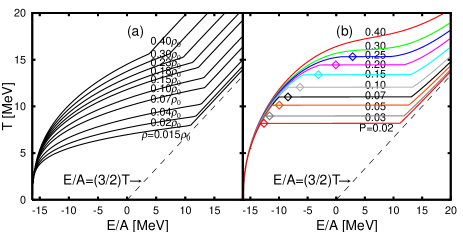
Figure 2: The caloric curves of infinite nuclear matter obtained by applying the Maxwell construction to the EOS (Fig. 1). The line of $E/A=(3/2)T$ is drawn for the comparison. (a) The constant volume caloric curves drawn for the average densities $\rho=0.40\rho_{0}$, $0.30\rho_{0}$, $0.23\rho_{0}$, $0.18\rho_{0}$, $0.15\rho_{0}$, $0.10\rho_{0}$, $0.07\rho_{0}$, $0.04\rho_{0}$, $0.02\rho_{0}$ and $0.015\rho_{0}$, where $\rho_{0}=0.17$ fm^-3 is the normal nuclear matter density. (b) The constant pressure caloric curves for the pressures $P=0.02$, 0.03, 0.05, 0.07, 0.10, 0.15, 0.20, 0.25, 0.30 and $0.40\,\text{MeV/fm}^{3}$. The meaning of the diamond marks is explained in Sec. V.3.

The obtained caloric curves with constant volume and with constant pressure are shown in Fig. 2(a) and Fig. 2(b), respectively. The existence of phase transition can be recognized in both caloric curves. However, only the constant pressure caloric curves show temperature plateau at coexistent region. The constant volume caloric curves show monotonic increase of temperature with the energy increase even in the coexistent region. Finding a temperature plateau in the constant pressure caloric curves is an easy way to identify first order phase transition in infinite systems.

In the realistic nuclear systems, however, the number of nucleons is several hundred at most. We have to carefully treat these systems because the ideas for infinite systems sometimes can not be applied to such small systems. Nevertheless, Gross et al. grossPR ; grossPCCP ; grossEP have pointed out that the essence of phase transition is the anomalous concavity of the entropy $S(E)=\ln W(E)$, with $W(E)$ being the number of microstates, and the effect of phase transition can be clearly observed even in finite systems by finding backbending (negative heat capacity) in the microcanonical caloric curves.

III Framework

The microcanonical ensemble with energy $E$, volume $V$ and particle number $A=N+Z$ can be obtained by solving the time evolution of the many-nucleon system confined in a container and regarding the state at each time as a sample of the ensemble. For the time evolution calculation, we utilize AMD, which is a microscopic dynamical model based on the degrees of freedom of interacting nucleons onoPRL ; onoPTP ; onoReview . AMD uses a fully antisymmetrized product of Gaussian wave packets,

$$\langle\mathbf{r}_{1}\ldots\mathbf{r}_{A}|\Phi(Z)\rangle=\det_{ij}\Bigl{[}\exp\Bigl{\{}-\nu\Bigl{(}\mathbf{r}_{j}-\frac{\mathbf{Z}_{i}}{\sqrt{\nu}}\Bigr{)}^{2}\Bigr{\}}\chi_{\alpha_{i}}(j)\Bigr{]},$$ (1)

where the complex variables $Z=\{\mathbf{Z}_{i};\ i=1,\ldots,A\}$ represent the centroids of the nucleon wave packets. The width parameter $\nu$ is treated as a constant parameter and taken as $\nu=0.16\;\text{fm}^{-2}$ so as to reasonably describe the ground state of light nuclei such as ${}^{16}\text{O}$. The spin-isospin states ($\chi_{\alpha_{i}}=p\uparrow$, $p\downarrow$, $n\uparrow$, and $n\downarrow$) are also independent of time. Because of the antisymmetrization, an AMD wave function $|\Phi(Z)\rangle$ contains many quantum features so that it is even utilized for the study of nuclear structures enyo .

The time evolution of the centroids $Z$, which parameterize $|\Phi(Z)\rangle$, is determined by a stochastic equation of motion

$$\frac{d}{dt}\mathbf{Z}_{i}=\{\mathbf{Z}_{i},\mathcal{H}\}+\Delta\mathbf{Z}_{i},$$ (2)

where $\{\mathbf{Z}_{i},\mathcal{H}\}$ is the deterministic term derived from the time-dependent variational principle and $\Delta\mathbf{Z}_{i}$ is the stochastic term, which is important to describe the appearance of various reaction channels in multifragmentation, for example. The stochastic term $\Delta\mathbf{Z}_{i}$ is also essential for the consistency with the quantum statistics ohnishiPRL ; ohnishiAP ; onoAMDMF ; onoSts . Two origins of the stochastic term $\Delta\mathbf{Z}_{i}$ are considered; one is the two-nucleon collisions and the other is related to the unrestricted single-particle motion in the mean field and the localization of single-particle wave functions when fragments are formed onoAu ; onoWithFrance ; onoReview .

In the following subsections, we briefly explain these terms referring to Refs. onoAu ; onoWithFrance ; onoReview . In this paper, we introduce several new improvements which are necessary for the present application because the energy conservation and the motion of emitted nucleons should be treated very consistently.

III.1 AMD time evolution

III.1.1 Deterministic part of the equation of motion

The deterministic term is derived from the time-dependent variational principle and given by

$$\{Z_{i\sigma},\mathcal{H}\}=\frac{1}{i\hbar}\sum_{j\tau}C^{-1}_{i\sigma,j\tau}\frac{\partial\mathcal{H}}{\partial Z^{\ast}_{j\tau}},$$ (3)

where

$$C_{i\sigma,j\tau}=\frac{\partial^{2}}{\partial Z^{\ast}_{i\sigma}\partial Z_{j\tau}}\ln\langle\Phi(Z)|\Phi(Z)\rangle$$ (4)

with $\sigma,\tau=x,y,z$ onoPRL ; onoPTP ; onoReview . The derived equation contains the expectation value of the effective Hamiltonian $\mathcal{H}$, which is given by

$$\mathcal{H}(Z)=\frac{\langle\Phi(Z)|H|\Phi(Z)\rangle}{\langle\Phi(Z)|\Phi(Z)\rangle}+\mathcal{K}_{\text{mod}}(Z)+\mathcal{V}_{\text{mod}}(Z).$$ (5)

Equation (5) contains the modification terms $\mathcal{K}_{\text{mod}}(Z)$ and $\mathcal{V}_{\text{mod}}(Z)$ for the kinetic and potential energies, respectively, both of which are for the treatment of the gaseous nucleons. If a nucleon is located out of nuclei and there are almost no other nucleons around it, the wave function of such a nucleon is interpreted to have a sharp momentum distribution rather than the momentum distribution corresponding to the Gaussian wave packet in Eq. (1). This change of interpretation has been necessary for the consistency of Q-values of nucleon emission and fragmentation onoPTP ; onoPRL ; onoReview , and is very important for the definition of temperature in the present work. By this modification, the zero-point kinetic energies of gaseous nucleons are subtracted from the total kinetic energy onoPTP ; onoPRL ; onoReview by

$$\mathcal{K}_{\text{mod}}(Z)=-\frac{3\hbar^{2}\nu}{2M}A+T_{0}(A-\mathcal{N}_{F}(Z)),$$ (6)

where the zero-point kinetic energies of isolated fragments are also subtracted. The function $\mathcal{N}_{F}(Z)$ stands for the number of isolated fragments and nucleons which are assumed to have the definite center-of-mass momenta without zero-point energies. Therefore we take $T_{0}(A-\mathcal{N}_{F})$ as the physical zero-point kinetic energy instead of $(3\hbar^{2}\nu/2M)A$. The functional form of $\mathcal{N}_{F}(Z)$ is given in Appendix A. The parameter $T_{0}$ should be $3\hbar^{2}\nu/2M$ in principle, but it may be adjusted to fine-tune the binding energies of nuclei. With the Gogny force, the binding energies for a wide range of nuclear chart are reproduced reasonably well by taking $T_{0}=9.20$ MeV which is close to $3\hbar^{2}\nu/2M=10.0$ MeV onoC12 ; onoReview . In Appendix A, the degree of isolation $\mathcal{I}_{i}$ for a nucleon $i$ is introduced. Using $\mathcal{I}_{i}$, the total zero-point kinetic energy can be written as

$$T_{0}(A-\mathcal{N}_{F})=T_{0}\sum_{i=1}^{A}(1-\mathcal{I}_{i})$$ (7)

so that the physical zero-point kinetic energy associated to the nucleon $i$ may be considered as $T_{0}(1-\mathcal{I}_{i})$. The potential energy should be also modified following the same change of interpretation of gaseous nucleons, because the spatial distribution of each gaseous nucleon is wide correspondingly to the sharp momentum distribution. The details of the modification term $\mathcal{V}_{\text{mod}}(Z)$ are also given in Appendix A. The parameters of the modification terms are chosen in such a way that a nucleon is treated as a gaseous nucleon (with a sharp momentum width) if the number of other nucleons around it is less than about 2. The binding energies of small nuclei such as deuteron and triton are utilized to fix some parameters.

Equation (5) defines the total energy that is to be conserved by the deterministic term $\{\mathbf{Z}_{i},\mathcal{H}\}$. The same energy is conserved also by the stochastic term. However, we need to be careful in treating the term $\mathcal{K}_{\text{mod}}(Z)$ because the force $-T_{0}\{\mathbf{Z}_{i},\mathcal{N}_{F}\}$ originating from this term is not always physically reasonable (see Sec. III.1.4).

III.1.2 Stochastic treatment of single particle motion

The stochastic term $\Delta\mathbf{Z}_{i}$ in Eq. (2) consists of two contributions. The first one is the stochastic two-nucleon collision term onoPRL ; onoPTP ; onoReview which is not shown explicitly in the following formulation for simplicity. The second one is related to the change of the phase space distribution by the mean field propagation. We follow the formalism of AMD/DS given in Refs. onoWithFrance ; onoReview , but also introduce new improvements which are crucial in the present study.

We write the Wigner function of the nucleon $k$ as the mean of the stochastic phase space distributions of deformed Gaussian shape,

$$f_{k}(x,t) =\overline{g(x;X_{k}(t),S_{k}(t))}$$ (8)

$$=\int{g(x;X,S)w_{k}(X,t)\frac{d^{6}X}{\pi^{3}}}$$ (9)

with

$$g(x;X,S)=\frac{1}{8\sqrt{\det S}}\\ \times\exp{\Bigl{[}-\frac{1}{2}\displaystyle\sum_{a,b=1}^{6}S_{ab}^{-1}(x_{a}-X_{a})(x_{b}-X_{b})\Bigr{]}}.$$ (10)

We have introduced the 6-dimensional phase space coordinates

$$x=\{x_{a}\}_{a=1,\dots,6}=\left\{\sqrt{\nu}\mathbf{r},\;\frac{\mathbf{p}}{2\hbar\sqrt{\nu}}\right\}.$$ (11)

At an initial time, $f_{k}$ is represented by a single Gaussian wave packet $g(x;X_{k},S_{k})$ with $S_{kab}=\frac{1}{4}\delta_{ab}$ and the wave packet centroid $X_{k}$ is identified with the physical coordinate $\mathbf{W}_{k}$ onoPRL ; onoPTP ; onoReview ;

$$X=\{X_{ka}\}_{a=1,\dots,6}=\left\{\text{Re}\mathbf{W}_{k},\;\text{Im}\mathbf{W}_{k}\right\}.$$ (12)

For a short time, the time evolution of $g_{k}(x,t)\equiv g(x;X_{k}(t),S_{k}(t))$ by the Vlasov equation

$$\frac{\delta g_{k}}{\delta t}=-\frac{\partial h}{\partial\mathbf{p}}\cdot\frac{\partial g_{k}}{\partial\mathbf{r}}+\frac{\partial h}{\partial\mathbf{r}}\cdot\frac{\partial g_{k}}{\partial\mathbf{p}},$$ (13)

is characterized by the time evolution of the first and the second moments of the distribution

$$\frac{\delta}{\delta t}X_{ka}(t) =\frac{\delta}{\delta t}\int{x_{a}g_{k}(x,t)\frac{d^{6}x}{\pi^{3}}},$$ (14)

$$\frac{\delta}{\delta t}S_{kab}(t) =\frac{\delta}{\delta t}\int{\!\!(x_{a}-X_{ka}(t))(x_{b}-X_{kb}(t))g_{k}(x,t)\frac{d^{6}x}{\pi^{3}}},$$ (15)

in which $(\delta/\delta t)g_{k}(x,t)$ is given by Eq. (13). A special notation of the time derivative $(\delta/\delta t)$ is adopted for the mean field propagation. The mean distribution [Eq. (9)] does not change when a part of the time evolution of the shape $S_{kab}$ is converted into a stochastic Gaussian fluctuation $\Delta X_{ka}(t)$ to the centroid $X_{ka}(t)$ as

$$\frac{d}{dt}X_{ka}(t) =\frac{\delta}{\delta t}X_{ka}(t)+\Delta X_{ka}(t)$$ (16)

$$\overline{\Delta X_{ka}(t)}=0,$$ (17)

$$\overline{\Delta X_{ka}(t)\Delta X_{kb}(t^{\prime})}=D_{kab}(t)\delta(t-t^{\prime}),$$ (18)

where $D_{kab}(t)$ denotes the strength and correlation of fluctuations. Correspondingly, the equation of motion for $S_{kab}(t)$ is given by

$$\frac{d}{dt}S_{kab}(t) =\frac{\delta}{\delta t}S_{kab}(t)-D_{kab}(t).$$ (19)

In order that the Vlasov equation is satisfied, the choice of $D_{kab}(t)$ is arbitrary as far as the positive definiteness of $D_{kab}(t)$ and $S_{kab}(t)$ is guaranteed.

In the original version of AMD/DS in Refs. onoWithFrance ; onoReview , $D_{kab}$ was chosen as the component diffusing beyond the original width of the wave packet, that is,

$$D^{(1)}_{kab}(t)=\lim_{\Delta t\rightarrow 0}\frac{1}{\Delta t}\sum_{c}\max\left(0,\;\lambda_{c}-\frac{1}{4}\right)O_{ac}O_{bc},$$ (20)

where $O_{ab}$ and $\lambda_{a}$ are the diagonalizing orthogonal matrix and the eigenvalues of the symmetric matrix $S_{k}(t)+\frac{\delta}{\delta t}S_{k}\Delta t$. With this original choice, however, there is no accordance between the momentum spreading of the distribution $S_{k}$ and the zero-point kinetic energy $T_{0}(1-\mathcal{I}_{k})$ assumed in the conserved energy (Sec. III.1.1). This accordance is important for the full consistency of the energy conservation and the precise evaluation of the temperature in the present work. Therefore we utilize the arbitrariness of $D$ and introduce another choice $D=D^{(1)}+D^{(2)}$ by adding a term $D^{(2)}$ as explained below.

Ignoring the effect of antisymmetrization for simplicity, the expectation value of the kinetic energy of an emitted nucleon $k$ can be written as

$$\mathcal{K}_{\text{hamil}}=\frac{2\hbar^{2}\nu}{M}(X_{k4}^{2}+X_{k5}^{2}+X_{k6}^{2})+T_{0}(1-\mathcal{I}_{k}),$$ (21)

which is a part of the conserved energy $\mathcal{H}$ and includes the zero-point kinetic energy. On the other hand, if we use the phase space distribution $g(x;X_{k},S_{k})$, the kinetic energy is given by

$$\mathcal{K}_{\text{distr}}=\frac{2\hbar^{2}\nu}{M}(X_{k4}^{2}+X_{k5}^{2}+X_{k6}^{2})+\frac{4}{3}T_{0}\mathop{\mathrm{Tr}_{p}}S_{k},$$ (22)

where ($3\hbar^{2}\nu/2M$) has been replaced by $T_{0}$ consistently with Eq. (6) and a special notation $\mathop{\mathrm{Tr}}_{p}S_{k}\equiv S_{k44}+S_{k55}+S_{k66}$ has been used. If only $D^{(1)}$ is taken, $(1-\mathcal{I}_{k})$ usually decreases faster than $\frac{4}{3}\mathop{\mathrm{Tr}}_{p}S_{k}$, when the nucleon $k$ is going out of a nucleus. Therefore, in order to keep the accordance of $\mathcal{K}_{\text{hamil}}$ and $\mathcal{K}_{\text{distr}}$, we choose $D_{k}$ so as to satisfy the condition

$$\mathop{\mathrm{Tr}_{p}}S_{k}=\frac{3}{4}(1-\mathcal{I}_{k}),$$ (23)

when the right hand side is getting smaller than the left hand side. This requirement can be satisfied by scaling $S_{kab}$ as

$$S_{kab}(t+\Delta t)=R_{k}S^{\prime}_{kab}$$ (24)

by a factor

$$R_{k}=\text{min}\left\{\frac{\frac{3}{4}(1-\mathcal{I}_{k})}{\mathop{\mathrm{Tr}_{p}}S^{\prime}_{k}},\;1\right\},$$ (25)

where $S^{\prime}_{kab}=S_{kab}(t)+(\frac{\delta}{\delta t}S_{kab}-D^{(1)}_{kab})\Delta t$. This corresponds to taking the choice $D_{kab}(t)=D^{(1)}_{kab}(t)+D^{(2)}_{kab}(t)$ with

$$D^{(2)}_{kab}(t)=\lim_{\Delta t\rightarrow 0}\frac{1}{\Delta t}(1-R_{k})S^{\prime}_{kab}.$$ (26)

III.1.3 Decoherence process

The fluctuation $\Delta X$ has been introduced in Eq. (16) by the condition that the single-particle dynamics of the mean field propagation would be reproduced. However, the mean field propagation is not sufficient to approximate the time evolution of many-body systems, at least, in the sense that the idempotency of the one-body density matrix ($\hat{\rho}^{2}=\hat{\rho}$) is unphysically kept during the mean field propagation. After enough time has past in the multifragmentation reactions, for example, the reduced one-body density matrix would be rather represented by an ensemble of density matrices in each of which single-particle wave functions are localized in fragments. This means that the coherence of the single-particle state is lost at some time (quantum branching). The decoherence is due to the many-body correlations and therefore its time scale (coherence time $\tau_{0}$) should be related to many-body effects in some way.

In Refs. onoWithFrance ; onoReview , the decoherence is assumed to take place for a nucleon when it is scattered by a two-nucleon collision, which is the effect beyond mean field. In the present calculation, however, we choose a different prescription to investigate the dependence on the decoherence process.

For each nucleon $k$, if there are more than three other nucleons within the radius of 2 fm (measured in $\mathop{\mathrm{Re}}\mathbf{W}/\sqrt{\nu}$), a decoherence process is assumed to take place with the probability of $1/\tau_{0}$ per unit time. When a decoherence process takes place, it affects all the nucleons $i$ that are located within the radius of 2 fm including the nucleon $k$ itself and each of the single particle wave packet of the nucleon $i$ is replaced by a Gaussian wave packet with the phase space distributions

$$S_{iab}=\begin{cases}\frac{1}{4}&(a=b=1,2,3)\\ \frac{1}{4}(1-\mathcal{I}_{i})&(a=b=4,5,6)\\ 0&(a\neq b)\end{cases}.$$ (27)

The momentum widths are replaced by $\frac{1}{4}(1-\mathcal{I}_{i})$ rather than the standard Gaussian width $\frac{1}{4}$ in order to satisfy Eq. (23). It should be noted that a single decoherence process affects several nucleons at once and therefore the rate of decoherence for a specific nucleon is approximately proportional to the number of the neighboring nucleons. We take $\tau_{0}=500$ fm/$c$ for usual calculations in the present work, but we also check the dependence of the results on $\tau_{0}$ in Sec. V.3.

III.1.4 The stochastic equation of motion

The stochastic equation of motion for the wave packet centroids $Z$ is given by onoAu ; onoReview

$$\frac{d}{dt}\mathbf{Z}_{i} =\{\mathbf{Z}_{i},\mathcal{H}\}+\sum_{k=1}^{A}\Bigr{(}(\Delta\mathbf{Z}_{i})^{(k)}_{\text{flct}}+(\Delta\mathbf{Z}_{i})^{(k)}_{\text{dssp}}\Bigr{)},$$ (28)

$$(\Delta\mathbf{Z}_{i})^{(k)}_{\text{flct}}=\left\{\mathbf{Z}_{i},\;\mathcal{O}^{\prime}_{k}+T_{0}\mathcal{I}_{k}\right\}_{\mathrm{C}_{k}},$$ (29)

$$(\Delta\mathbf{Z}_{i})^{(k)}_{\text{dssp}}=\mu_{k}\left(\mathbf{Z}_{i},\mathcal{H}^{\prime}\right)_{\mathrm{N}_{k}}.$$ (30)

The fluctuation term $(\Delta\mathbf{Z}_{i})^{(k)}_{\text{flct}}$ is obtained by converting the fluctuation $\Delta X_{ka}$ of the physical coordinate $W$ to that of the original AMD coordinates $Z$. This conversion is done onoReview ; onoAu by introducing an expectation value $\mathcal{O}_{k}(Z,t)$ of a stochastic one-body operator which generates the fluctuation as $\{\mathbf{Z}_{i},\mathcal{O}_{k}\}$ by the Poisson brackets [Eq. (3)]. $\mathcal{O}^{\prime}_{k}$ in Eq. (30) is different from $\mathcal{O}_{k}$ by the Lagrange multiplier terms for the conservation of the three components of the center-of-mass coordinate and those of the total momentum onoReview ; onoAu . The term $T_{0}\{\mathbf{Z}_{i},\mathcal{I}_{k}\}$ in $(\Delta\mathbf{Z}_{i})^{(k)}_{\text{flct}}$ is introduced in order to cancel the unphysical force $-T_{0}\{\mathbf{Z}_{i},\mathcal{I}_{k}\}$ in the deterministic term $\{\mathbf{Z}_{i},\mathcal{H}\}$. Such a force does not exist for the single-particle motion in the mean field one-body dynamics. The subtraction is introduced as a term in $(\Delta\mathbf{Z}_{i})^{(k)}_{\text{flct}}$ for a technical reason (related to the dssp term) so that the Hamiltonian $\mathcal{H}$ with the zero-point correction term $T_{0}(1-\mathcal{I}_{k})$ is still the conserved energy.

The term $(\Delta\mathbf{Z}_{i})^{(k)}_{\text{dssp}}$ is the dissipation term to achieve the energy conservation, where $(Z_{i\sigma},\mathcal{H}^{\prime})$ is defined by

$$(Z_{i\sigma},\mathcal{H}^{\prime})=\frac{1}{\hbar}\sum_{j\tau}C^{-1}_{i\sigma,j\tau}\frac{\partial\mathcal{H}^{\prime}}{\partial Z^{\ast}_{j\tau}}.$$ (31)

The coefficient $\mu_{k}$ for each $k$ is determined so that the energy violation by the $(\Delta\mathbf{Z}_{i})^{(k)}_{\text{flct}}$ term is compensated by $(\Delta\mathbf{Z}_{i})^{(k)}_{\text{dssp}}$. Lagrange multiplier terms are included in the effective Hamiltonian $\mathcal{H}^{\prime}$, assuming that $(\Delta\mathbf{Z}_{i})^{(k)}_{\text{dssp}}$ conserves some global one-body quantities such as the center-of-mass coordinate, the total momentum, the total orbital angular momentum, and the monopole and quadrupole moments in the coordinate and momentum spaces onoAu ; onoReview .

The subscripts $\mathrm{C}_{k}$ and $\mathrm{N}_{k}$ mean that the contents of the brackets are calculated by limiting to the subsystem $\mathrm{C}_{k}$ or $\mathrm{N}_{k}$. $\mathrm{C}_{k}$ is the cluster that includes the nucleon $k$, where the clusters are identified by the condition that two nucleons $i$ and $j$ belong to the same cluster if $|\mathbf{Z}_{i}-\mathbf{Z}_{j}|<1.75$. $\mathrm{N}_{k}$ stands for a neighborhood of nucleon $k$ defined by

$$\mathrm{N}_{k} =\{i;\;|\mathbf{W}_{i}-\mathbf{W}_{k}|<2.5,i\in\mathrm{C}_{k},i\neq k,\ \mbox{and}\ M_{i}>1\},$$ (32)

where $M_{i}$ is the number of nucleons within the distance of 3 fm (measured in $\mathop{\mathrm{Re}}\mathbf{W}/\sqrt{\nu}$) from nucleon $i$. These limitations ensure that the fluctuation $X_{ka}$ for the nucleon $k$ should affect only the nucleons within the interactive range of the nucleon $k$ when the conservation laws are imposed. The condition $M_{i}>1$ in Eq. (32) is introduced to exclude gaseous nucleons (here we regard the nucleon $i$ with $M_{i}\leq 1$ as gaseous) from $\mathrm{N}_{k}$ so that the dynamics of the gaseous nucleon $i$ faithfully follows the single-particle motion determined by the deterministic term $\{\mathbf{Z}_{i},\mathcal{H}\}$ and the fluctuation term $\sum_{k=1}^{A}(\Delta\mathbf{Z}_{i})_{\text{flct}}^{(k)}$. The choice of $\mathrm{C}_{k}$ and $\mathrm{N}_{k}$ here is similar to Refs. onoAu ; onoReview , but has been updated in order to carefully treat gaseous nucleons, which is required for the precise definition of temperature.

We cancel the fluctuation for a nucleon $k$ when the number of nucleons in $\mathrm{N}_{k}$ is less than five to prevent small clusters from unphysically breaking.

III.2 Reflection at the wall

To obtain a microcanonical ensemble with a fixed volume, we need to keep nucleons inside the container with a given volume $V=\frac{4\pi}{3}r^{3}_{\text{wall}}$ during the time evolution. We introduce a kind of reflection process for this purpose, when nucleons or fragments are going out of the container. At each time step after the time evolution without any effect of the container wall, we judge whether each nucleon $k$ is in the container ($\frac{1}{\sqrt{\nu}}|\text{Re}\mathbf{W}_{k}|\leq r_{\text{wall}}$). If an isolated nucleon $k$ is located outside the container and its momentum $\mathbf{P}_{k}=2\hbar\sqrt{\nu}\text{Im}\mathbf{Z}_{k}$ directs outward, we change the momentum direction $\hat{\mathbf{P}}_{k}=\mathbf{P}_{k}/|\mathbf{P}_{k}|$ into an inward direction $\hat{\mathbf{P}}^{\prime}_{k}$ which satisfies $\mathbf{R}_{k}\cdot\hat{\mathbf{P}}^{\prime}_{k}<0$, where $\mathbf{R}_{k}=\frac{1}{\sqrt{\nu}}\mathrm{Re}\mathbf{Z}_{k}$. We randomly choose the direction $\hat{\mathbf{P}}^{\prime}_{k}$ as in the case of the reflection by an irregular surface. The absolute value of the momentum $|\mathbf{P}^{\prime}_{k}|$ is adjusted so as to conserve the total energy which is sometimes affected by antisymmetrization. The total angular momentum of the system is not conserved because of the irregular reflection, which allows us to construct a microcanonical ensemble without the constraint of the total angular momentum.

When a nucleon which belongs to a cluster, where we regard the nucleon $i$ and $j$ belong to the same cluster when $|\mathbf{W}_{i}-\mathbf{W}_{j}|<0.8$, is located outside the container, we apply a similar reflection procedure to the center of mass coordinate of the cluster. If one applied the reflection procedure to each of the nucleons in the cluster as is done in Refs. ohnishiPRL ; ohnishiAP ; FMDLGpt ; onoAMDMF ; onoSts ; sugawaVolkov ; sugawaGogny , the cluster would be unphysically broken by the crash to the wall.

When a nucleon $k$ is reflected, the shape $S_{k}$ has to be reflected consistently with the change of the momentum direction $\hat{\mathbf{P}}_{k}\to\hat{\mathbf{P}}^{\prime}_{k}$. We consider the reflection with respect to the plane that includes the point $\mathbf{R}_{k}$ and is perpendicular to $\hat{\mathbf{n}}_{k}=(\hat{\mathbf{P}}^{\prime}_{k}-\hat{\mathbf{P}}_{k})/|\hat{\mathbf{P}}^{\prime}_{k}-\hat{\mathbf{P}}_{k}|$, and hence the component parallel to $\hat{\mathbf{n}}_{k}$ is reversed. According to this operation, the coordinate or momentum vector $\mathbf{x}_{k}$ in the intrinsic frame of the wave packet $k$ is transformed into

$$\mathbf{x}^{\prime}_{k}=\mathbf{x}_{k}-2\left(\mathbf{x}_{k}\cdot\hat{\mathbf{n}}_{k}\right)\hat{\mathbf{n}}_{k}=T_{k}\;\mathbf{x}_{k},$$ (33)

$$(T_{k})_{\sigma\tau}=\delta_{\sigma\tau}-2n_{k\sigma}n_{k\tau}\quad(\sigma,\tau=x,y,z).$$ (34)

By defining the transformation matrix in the phase space as

$$\mathcal{T}_{k}=\begin{pmatrix}T_{k}&0\\ 0&T_{k}\end{pmatrix},$$ (35)

the transformation of the shape $S_{k}$ is given by

$$S^{\prime}_{kab}=\sum_{cd}(\mathcal{T}_{k})_{ac}(\mathcal{T}_{k})_{bd}S_{kcd}.$$ (36)

In the actual calculation, for the purpose of numerical stability, we introduce a small delay time $\tau_{\text{delay}}$ for the response to the fluctuation $\Delta X_{ka}$ onoAu ; onoReview . This delayed fluctuation $\Xi_{ka}(t)$ also has to be transformed as $\Xi^{\prime}_{ka}=\sum_{b}(\mathcal{T}_{k})_{ab}{\Xi}_{kb}$ when a nucleon $k$ is reflected.

IV Calculation of temperature and pressure

In order to obtain caloric curves, we need to extract the temperature $T$ of each microcanonical ensemble $\{E,V,A\}$. We also need to know the pressure $P$ of the ensemble in order to draw the constant pressure caloric curves. In this section, we explain how to obtain $T$ and $P$ in our calculation.

The microcanonical temperature is defined by $T^{-1}=(\partial S/\partial E)|_{V,A}$. This quantity can be evaluated with a good precision by using the average kinetic energy of gaseous nucleons. When the total volume is $V>A/\rho_{0}$, where $\rho_{0}=0.17$ fm^-3 is the normal nuclear density, it is possible to find a partial system composed of gaseous nucleons to which classical ideal gas relations are applicable. Let us call this partial system $\mathrm{G}$ which will be defined below. Appendix B shows that the microcanonical temperature $T$ of the ensemble $\{E,V,A\}$ can be obtained from the average kinetic energy of G-subsystem as

$$T=\frac{2}{3}\biggl{<}\frac{\mathcal{K}_{\mathrm{G}}}{A_{\mathrm{G}}}\biggr{>}_{\{E,V,A,A_{\mathrm{G}}>0\}},$$ (37)

where $\mathcal{K}_{\mathrm{G}}$ and $A_{\mathrm{G}}$ are the kinetic energy and the number of nucleons of G-subsystem, respectively, and the brackets $\langle\,\rangle_{\{E,V,A,A_{\mathrm{G}}>0\}}$ denote the average value for the microcanonical ensemble with $A_{\mathrm{G}}>0$. Because of the consistency of Eq. (21) and Eq. (22), $\mathcal{K}_{\mathrm{G}}$ can be calculated as

$$\mathcal{K}_{\mathrm{G}}=\sum_{k\in\mathrm{G}}\Bigl{\{}\frac{2\hbar^{2}\nu}{M}(X_{k4}^{2}+X_{k5}^{2}+X_{k6}^{2})+\frac{4}{3}T_{0}\mathop{\mathrm{Tr}_{p}}S_{k}\Bigr{\}}.$$ (38)

The first term is the contribution from the wave packet centroid. The accumulated delayed fluctuation $\tau_{\text{delay}}\mathbf{\Xi}_{k}$ onoAu should be included in this term because the corresponding shape shrinking has been already applied. The second term is the contribution from the momentum widths of $S_{k}$.

According to Appendix B, G-subsystem can be defined arbitrarily as far as the following two conditions are satisfied. The first condition is that the quantum effect should be negligible for any nucleon in G-subsystem. The second condition is that the G-subsystem should be selected without using momentum variables, i.e., the configurations with different nucleon momenta should be equally taken into account if they have the same nucleon positions.

In our actual calculation, G-subsystem has been chosen in the following way. We select the nucleons $k$ for which the density of the nucleons with the same spin-isospin

$$\rho_{\alpha}=\sum_{i\in\alpha_{k},i\neq k}\left(\frac{2\nu}{\pi}\right)^{3/2}e^{-2(\text{Re}\mathbf{W}_{k}-\text{Re}\mathbf{W}_{i})^{2}},$$ (39)

is sufficiently low ($\rho_{\alpha}\leq\rho_{\mathrm{G}}=(1/200)\rho_{0}$) so that the antisymmetrization effect can be neglected. It is necessary to eliminate the nucleons belonging to clusters because the discrete level(s) of the internal degrees of freedom can only be treated quantum mechanically. Therefore, among the selected nucleons, we choose the nucleons $k$ which do not have more than one other nucleon within the distance of $r_{\mathrm{G}}=3\,\text{fm}$ (if we use $M_{k}$ defined in Sec. III.1.2, we choose the nucleon $k$ which satisfy the condition $M_{k}\leq 1$). Because of our reflection procedure, it is possible that nucleons locate outside the container in short time interval. Those nucleons are excluded from the selected nucleons. The above selections are done based on spatial coordinates without any momentum selection. We define the system composed of these selected nucleons as G-subsystem. The results should be independent of the definition of G as far as the necessary conditions are respected, which will be checked in Sec. V.3 by changing the criteria in our definition of G.

For the calculation of the pressure $P$, we adopt the common definition of pressure as the external force necessary to keep the volume. Namely the pressure is given by

$$P=\frac{2}{4\pi r^{2}_{\text{wall}}\tau_{\text{total}}}\sum_{\text{reflections}}\Delta\mathbf{p}\cdot\hat{\mathbf{N}}$$ (40)

where the summation is taken over all the reflections at the container wall (see Sec. III.2) which occurred during the time evolution of the total time $\tau_{\text{total}}$, $\Delta\mathbf{p}$ is the momentum change at each reflection, and $\hat{\mathbf{N}}$ is the normal vector. Factor two is from the fact that when a nucleon or a fragment hits the wall the total momentum of the rest of the system is also changed for the momentum conservation.

V The studied system and obtained caloric curves

V.1 The studied system

In the present study, the system with $(N,Z)=(18,18)$ is considered, which is the same system taken in Refs. sugawaVolkov ; sugawaGogny . There are several examples indicating that phase transition exists even in such small systems schmidt ; gobet1 ; gobet2 .

Microcanonical ensembles are constructed with the radius of the container $r_{\text{wall}}=5$, $5.5,\dots,15$ fm, which correspond to the average densities $A/(\frac{4\pi}{3}r_{\text{wall}}^{3})=0.40\rho_{0}$, $0.30\rho_{0},\dots,0.015\rho_{0}$, and the energy $E^{\ast}/A=4,$ $\ 6,\dots,28$ MeV, where $E^{\ast}$ stands for the excitation energy relative to the ground state of ${}^{36}\text{Ar}$ nucleus ($E_{\text{g.s.}}=-8.9A$ MeV). The minimum radius $r_{\text{wall}}=5$ fm corresponds to a volume of the container $V=2.5A/\rho_{0}$, and therefore we do not consider a compressed liquid nucleus in this study.

The time evolution was calculated up to 20000 fm/$c$, which is much longer than a typical nuclear reaction time scale ($\sim 100$ fm/$c$). The states for the first 5000 fm/$c$ were discarded in order to remove the initial state dependence. Samplings were done at every 10 fm/$c$. Similar calculations were carried out 4 times independently to improve the statistics.

V.2 Obtained caloric curves

The obtained constant volume caloric curves with $r_{\text{wall}}=5$, 5.5, 6, 6.5, 7, 8, 9 and 11 fm are shown in Fig. 3.

Figure 3: The constant volume caloric curves for the $A=36$ system obtained by AMD. The lines correspond to the container size $r_{\text{wall}}=5$, 5.5, 6, 6.5, 7, 8, 9 and 11 fm from the top. Statistical uncertainty is shown by error bars. The line of $E/A=(3/2)T$ is drawn for comparison.

The caloric curves with $r_{\text{wall}}=13$ and 15 fm are also constructed, but they are not shown in Fig 3 because the complete equilibration could not be achieved by our investigation time (20000 fm/$c$) in the low energy cases ($E^{\ast}/A=4\sim 8$ MeV) [the results systematically differ if we start the calculation with a quite different initial state]. Otherwise, fairly smooth caloric curves are obtained. The negative heat capacity (backbending) or plateau does not appear in the constant volume caloric curves, which is consistent with the result of Ref. sugawaGogny with another version of AMD. It was expected from the fact that the constant volume caloric curves for infinite nuclear matter do not show the plateau even in coexistent region (Fig. 2(a)).

Although this result (Fig. 3) is somehow similar to the caloric curves for infinite matter (Fig. 2(a)), the transition from the liquid-gas phase coexistence to the pure gas phase is not clear. It is difficult to judge clearly whether the phase transition exist or not from the constant volume caloric curves. On the other hand, the constant pressure caloric curves which showed plateau in the case of infinite nuclear matter (Fig. 2(b)) are expected to show the signal of the liquid-gas phase transition most clearly. Therefore, the judgment should be done with the constant pressure caloric curve, not with the constant volume caloric curve.

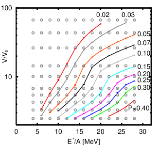
Figure 4: The constant pressure lines drawn on $E$-$V$ plain. The circles indicate the points where the microcanonical ensembles are constructed. The lines correspond to the constant pressure lines with $P=0.02$, 0.03, 0.05, 0.07, 0.10, 0.15, 0.20, 0.25, 0.30 and 0.40 MeV/fm³, which are obtained by performing the transformation between volume $V$ and pressure $P$ with the interpolation at each energy $E$. Statistical uncertainty is shown by error bars.

Constant pressure caloric curves can also be constructed from our results as follows. After the evaluation of all the ensembles $\{E,V,A\}$, we eventually know the temperature and the pressure at each lattice point on the $E$-$V$ plain indicated by circles in Fig. 4. From these results, we can draw constant pressure lines on the $E$-$V$ plain by performing the transformation between volume $V$ and pressure $P$ with the interpolation at each energy $E$. The obtained constant pressure lines are shown in Fig. 4. The relation between energy $E$ and temperature $T$ along these constant pressure lines corresponds to the constant pressure caloric curves. These caloric curves should not be confused with the caloric curves for the constant pressure ensemble $\{E,P,A\}$. The obtained caloric curves are those calculated from the microcanonical ensemble $\{E,V_{P},A\}$, where the volume $V_{P}$ is chosen so that the ensemble gives a certain pressure $P$.

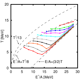
Figure 5: The constant pressure caloric curves for the $A=36$ system obtained by AMD. The lines correspond to the pressure $P=0.02$, 0.03, 0.05, 0.07, 0.10, 0.15, 0.20, 0.25, 0.30 and 0.40 MeV/fm³ from the bottom. Statistical uncertainty is shown by error bars. The curves of $E^{\ast}/A=T^{2}/(8\,\text{MeV})$ and $E^{\ast}/A=T^{2}/(13\,\text{MeV})$, and the line of $E/A=(3/2)T$ are drawn for comparison.

Figure 5 shows the constant pressure caloric curves with the pressure $P=0.02$, 0.03, 0.05, 0.10, 0.15, 0.20, 0.25, 0.30 and $0.40\;\text{MeV}/\text{fm}^{3}$ obtained by the above procedure. In each caloric curve with $P\lesssim 0.15$ MeV/$\text{fm}^{3}$, negative heat capacity is observed clearly, which is the signal of first order phase transition. For example at $P=0.05$ MeV/$\text{fm}^{3}$, the caloric curve start from $E^{\ast}/A=8$ MeV and the temperature decreases till the energy of 16 MeV even the system is heated up from 8 MeV to 16 MeV, and after the energy of 16 MeV, the temperature goes up with a slope 3/2. By the comparison with the infinite nuclear matter caloric curves (Fig. 2(b)), the caloric curves with $P<0.20$ MeV/$\text{fm}^{3}$ in Fig. 5 can be interpreted as the caloric curves drawn from the liquid-gas phase coexistence to the pure gas phase.

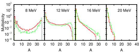
Figure 6: The fragment mass distributions along the $P=0.05$ MeV/fm³ line. Full lines are the distributions obtained with $r_{\text{clust}}=2.5$ fm. Dashed lines are the distributions obtained with $r_{\text{clust}}=3.0$ fm.

Figure 6 shows the fragment mass distributions for the ensembles along the $P=0.05$ MeV/fm³ line. Full lines are the distributions of the fragments identified by the condition that two nucleons $i$ and $j$ belong to the same cluster if $|\frac{1}{\sqrt{\nu}}\text{Re}(\mathbf{W}_{i}-\mathbf{W}_{j})|<r_{\text{clust}}=2.5$ fm. These distributions do not necessarily correspond to the fragments which would be emitted when the container wall is removed. In fact, the distributions change when $r_{\text{clust}}$ is varied. The dashed lines in Fig. 6 show the fragment mass distributions obtained with $r_{\text{clust}}=3.0$ fm. Nevertheless, these distributions are helpful for the qualitative understanding of the change of the system with energy increase. When the energy is low ($E^{\ast}/A=8$ MeV), the distribution shows U-shape with two peaks so that the typical configuration at this energy is a large nucleus coexisting with a few gaseous nucleons. When the energy is increased ($E^{\ast}/A=12\sim 16\,\text{MeV}$), the peak at the large fragment becomes smaller and the distribution changes into shoulder-like and power-low-like shapes. Thus complex configurations with many intermediate and light mass fragments are typical at these energies, and the proportion of light fragments increases as the energy increases (from $E^{\ast}/A=12\,\text{MeV}$ to 16 MeV). When the energy is sufficiently high ($E^{\ast}/A=20$ MeV), the distribution changes into exponential shape, which can be interpreted that the nucleons are moving almost freely at this energy, although a few nucleons come close and make compounds with small probability. The change of the distribution is fully consistent with the interpretation of the caloric curve, that is, the system along the $P=0.05$ MeV/fm³ line changes from liquid-gas phase coexistence at low energy to pure-gas phase at high energy.

The caloric curves in Fig. 5 do not contain the pure liquid phase because of our choice of the container size $r_{\text{wall}}\geq 5$ fm. Nevertheless, we can roughly guess the pure liquid caloric curve from our result as follows. Diamond marks in the constant pressure caloric curves for infinite nuclear matter (Fig. 2(b)) indicate the points corresponding to the density with $r_{\text{wall}}=5$ fm. These points are inside of the plateau region, but are very close to the left edge of the coexistence region. Furthermore, as is seen in Fig. 2(b), the pure liquid caloric curves are almost independent of the pressure unless the liquid is compressed with higher pressure ($P>0.3$ MeV/$\text{fm}^{3}$). We can guess the corresponding line by connecting the leftmost points of our AMD result and the line can be compared to the Fermi gas formula $E^{\ast}/A=aT^{2}$ for excited nuclei. The pure liquid caloric curve should be slightly left to the connected line. Thus our AMD result seems to be consistent with the quantum and fermionic statistics with a reasonable level density parameter $a^{-1}=8\sim 13$ MeV.

If we simply define the critical point as the point where the negative heat capacity disappears, the critical temperature and the critical pressure can be estimated as $T_{\mathrm{C}}\sim 12$ MeV and $P_{\mathrm{C}}\sim 0.20$ MeV/fm³, respectively. These values are lower than those of infinite nuclear matter ($T_{\mathrm{C}}\sim 16$ MeV and $P_{\mathrm{C}}\sim 0.3$ MeV/fm³). The lowering of $T_{\mathrm{C}}$ seems to be reasonable because the existence of the surface for fragments reduces the interaction energy gain by being fragments (liquid phase).

V.3 Check of the theoretical ambiguities

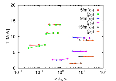
Figure 7: The temperatures obtained with different parameter sets ($r_{\mathrm{G}}$ and $\rho_{\mathrm{G}}$) for choosing G-subsystem. The results of the systems with $r_{\mathrm{wall}}=5,9,15$ fm and $E^{\ast}/A=6,14,22$ MeV are shown. The abscissa $\langle A_{\mathrm{G}}\rangle$ is the average number of nucleons in G-subsystem and the parameters are chosen so that $\langle A_{\mathrm{G}}\rangle$ becomes about half and about a quarter of the original choice [$r_{\mathrm{G}}=3$ fm and $\rho_{\mathrm{G}}=(1/200)\rho_{0}$]. The open points show the dependence of $r_{\mathrm{G}}$ and the solid points show the dependence of $\rho_{\mathrm{G}}$, which are connected by lines to guide eyes. Statistical uncertainty is similar to or smaller than the size of points.

As is mentioned in Sec. IV, the measured temperatures should be independent of the choice of G-subsystem as far as the conditions described in Sec. IV are satisfied. This can be checked by changing the criteria in the definition of G. In Sec. IV, G-subsystem has been selected as the subsystem of the nucleons which satisfy $\rho_{\alpha}\leq\rho_{\mathrm{G}}=(1/200)\rho_{0}$ and do not have more than one other nucleon within the distance of $r_{\mathrm{G}}=3\,\text{fm}$.

According to Appendix B, the dependence on $\rho_{\mathrm{G}}$ and $r_{\mathrm{G}}$ should be weak if only exist. This is actually demonstrated in Fig. 7 which shows the temperatures obtained with different choices of parameters ($r_{\mathrm{G}}$ and $\rho_{\mathrm{G}}$) to select G-subsystem. The parameters are chosen so that the average number of nucleons in G-subsystem $\langle A_{\mathrm{G}}\rangle$ becomes about half and about a quarter of the original choice. The open points show the dependence on $r_{\mathrm{G}}$ and the solid points show the dependence on $\rho_{\mathrm{G}}$. The temperatures are almost independent of the choice of the parameters. Only small dependence on the parameters can be noticed when $\langle A_{\mathrm{G}}\rangle\lesssim 1$. This is probably because we measure the temperature by using only the states with $A_{\mathrm{G}}>0$ (see Appendix B). Nevertheless, the dependence is very weak and seen only at low energy and at small volume so that the ambiguity associated with this issue would hardly affect the obtained results shown in Sec. V.2 and would not change the conclusions.

In the current AMD dynamical calculation, the coherence time $\tau_{0}$ (Sec. III.1.3) is somehow arbitrary. The above results (Figs. 3-7) are obtained with the choice $\tau_{0}=500\,\text{fm}/c$. We should check the robustness of the obtained results against the arbitrariness of the coherence time. Thus we have done the calculations with $\tau_{0}=250$ and $1000\,\text{fm}/c$. The obtained constant pressure caloric curves are shown in Fig 8(a) and Fig. 8(b), respectively.

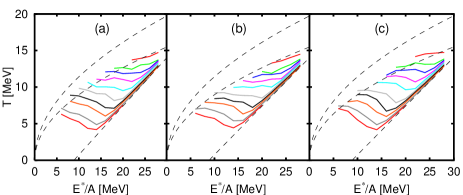
Figure 8: The AMD results of the constant pressure caloric curves with $P=0.02$, 0.03, 0.05, 0.10, 0.15, 0.20, 0.30 and 0.40 MeV/$\text{fm}^{3}$ from the bottom when the coherence time is varied: (a) $\tau_{0}=250$ fm/c, (b) $\tau_{0}=1000$ fm/c, (c) the same procedure as in Refs. onoWithFrance ; onoReview .

Furthermore, we have done the calculation with another choice of the decoherence process adopted in Refs. onoWithFrance ; onoReview and the obtained constant pressure caloric curves are shown in Fig. 8(c). By the comparison of the figures in Fig. 8 and Fig. 5, we notice some change of the leftmost point of each caloric curve, which can be interpreted as the change of the level density parameter $a$ for the liquid caloric curve. This dependence limits the possible range of the coherence time $\tau_{0}$ when the level density parameter $a$ is known. In any case, negative heat capacity is observed in all the caloric curves for a wide range of $\tau_{0}$.

VI Summary

In this paper, we have constructed the microcanonical caloric curves of a system with 36 nucleons [$(N,Z)=(18,18)$] using the microscopic time evolution of AMD. We applied the same AMD model that has been applied to nuclear reactions successfully.

For the first time as a molecular dynamics calculation for nuclear systems, we have constructed the constant pressure caloric curves and found that negative heat capacity appears there with an appropriate nuclear force (the Gogny force). Negative heat capacity (backbending) is a specific character of first order phase transition in finite systems. Thus we confirm the existence of nuclear liquid-gas phase transition under the ideal thermal equilibrium condition with AMD. The obtained fragment mass distributions also support the existence of the phase transition. We have checked that the extracted temperature from the ensembles do not change when different criteria to choose the nucleons for the temperature measurement are used as long as necessary conditions are satisfied. We have also checked the obtained conclusions are insensitive to the theoretical ambiguity, i.e. the coherence time $\tau_{0}$. The critical temperature and the critical pressure are estimated as $T_{C}\sim 12$ MeV and $P_{C}\sim 0.20$ MeV/fm³, but these values may slightly depend on the choice of $\tau_{0}$. As for a future study, it is interesting to investigate the dependence of the backbending and the critical point on the size and the isospin composition of the system.

We have also shown constant volume caloric curves, but the signal of the phase transition can not be seen clearly there. It suggests that it is important to identify the path of caloric curves drawn on $E$-$V$ plain when those are constructed from experimental data to discuss the existence of nuclear liquid-gas phase transition.

As we have demonstrated in this paper, AMD can be applied to ideal thermal equilibrium situations as well as the dynamical processes of the reactions. Therefore, it may be possible to construct the method to extract the statistical information from experimental data by studying the reaction simulation results of AMD together with the calculations of ideal systems in thermal equilibrium.

Appendix A The modification of the energy for gaseous nucleons

The fragment number $\mathcal{N}_{F}$ utilized in this paper is similar to the one in Ref. onoC12 , but a small modification is introduced. The fragment number of Ref. onoC12 was defined as

$$\mathcal{N}^{(0)}_{F}=\sum^{A}_{i=1}\mathcal{I}^{(0)}_{i},\quad\mathcal{I}^{(0)}_{i}=\frac{g(k_{i})}{n_{i}m_{i}},$$ (41)

where

$$n_{i}=\sum_{j=1}^{A}\hat{f}_{ij},\;m_{i}=\sum_{j=1}^{A}\frac{1}{n_{j}}f_{ij},\;k_{i}=\sum_{j=1}^{A}\bar{f}_{ij},$$ (42)

and

$$\hat{f}_{ij}=F(d_{ij},\hat{\xi},\hat{a}),\;f_{ij}=F(d_{ij},\xi,a),\;\bar{f}_{ij}=F(d_{ij},\bar{\xi},\bar{a}),$$ (43)

$$d_{ij}=|\text{Re}(\mathbf{Z}_{i}-\mathbf{Z}_{j})|,$$ (44)

$$F(d,\xi,a)=\begin{cases}1&(d\leq a)\\ e^{-\xi(d-a)^{2}}&(d>a)\end{cases},$$ (45)

$$g(k)=1+g_{0}e^{-(k-M)^{2}/2\sigma}.$$ (46)

$$\xi$$

2.0 0.6 2.0 0.2 1.0 0.5 1.0 2.0 12

(49)

In the present study, a gaseous nucleon is counted as a separate ‘fragment’ for the convenience of the temperature measurement. We allow a few gaseous nucleons get spatially close by regarding the nucleon $i$ as gaseous when the number of the neighboring nucleons including itself

$$q_{i}=\sum_{j=1}^{A}f_{ij}$$ (50)

is less than about three. This description is achieved by defining the fragment number $\mathcal{N}_{F}$ as

$$\mathcal{N}_{F}=\sum_{i=1}^{A}\mathcal{I}_{i},\quad\mathcal{I}_{i}=(1-w(q_{i}))\mathcal{I}^{(0)}_{i}+w(q_{i}),$$ (51)

where

$$w(q)=F(q,1/2\sigma_{q}^{2},Q)$$ (52)

and the parameters are taken as $\sigma_{q}=0.85$ and $Q=2.5$. The newly introduced function $w(q_{i})$ becomes zero unless $q\lesssim Q$ and the degree of isolation $\mathcal{I}_{i}$ reduces to the original one $\mathcal{I}^{(0)}_{i}$. On the other hand, $\mathcal{I}_{i}$ becomes close to one for the nucleons with $q_{i}\lesssim Q$.

The potential energies between the gaseous nucleons ($q_{i}\lesssim Q$) are also modified in the present study. The term $\mathcal{V}_{\text{mod}}$ of Eq. (5) is introduced for this purpose. The potential energy between two gaseous nucleons is calculated by folding the widely spread wave functions with their interaction. The spread wave function, keeping the centroid position in coordinate and momentum space same as the original Gaussian wave function [Eq. (1)], is given by

$$\phi_{i}(\mathbf{r};\alpha)=\left(\frac{2\nu}{\pi(1+\alpha)}\right)^{\frac{3}{4}}\exp\left[-\frac{\nu}{1+\alpha}(\mathbf{r}-\frac{\mathbf{Z}^{\prime}_{i}}{\sqrt{\nu}})^{2}\right]$$ (53)

$$\mathbf{Z}^{\prime}_{i}=\text{Re}\mathbf{Z}_{i}+i(1+\alpha)\text{Im}\mathbf{Z}_{i},$$ (54)

where $\alpha$ is a smearing parameter. By denoting the potential energy between nucleon $i$ and nucleon $j$ as $\mathcal{V}_{ij}$ calculated with the original Gaussian [Eq. (1)] and $\mathcal{V}_{ij}(\alpha)$ calculated with the smeared Gaussian [Eq. (53)], $\mathcal{V}_{\text{mod}}$ is given by

$$\mathcal{V}_{\text{mod}}=\sum_{i<j}^{A}w(q_{i})w(q_{j})\Bigl{[}-\mathcal{V}_{ij}+\mathcal{V}_{ij}(\alpha)\Bigr{]}.$$ (55)

The smearing parameter is chosen as $\alpha=3$ in order to reasonably reproduce the binding energies of small nuclei such as deuteron, triton and ${}^{3}\textrm{He}$ in case those stable compounds are formulated during dynamical processes. The density-dependent part of the effective interaction is also included in $\mathcal{V}_{\text{mod}}$ with a similar approximation used in the triple-loop approximation onoAu . When we evaluate $V_{ij}(\alpha)$ with the density-dependent part, we have also modified the density $\rho(\mathbf{r})$ consistently with the transformation of the wave function [Eq. (53)] as

$$\rho(\mathbf{r};\alpha)=\int\left(\frac{2\nu}{\pi\alpha}\right)^{\frac{3}{2}}e^{-(2\nu/\alpha)(\mathbf{r}-\mathbf{r}^{\prime})^{2}}\rho(\mathbf{r}^{\prime})d^{3}r^{\prime}.$$ (56)

Appendix B Temperature calculation by gaseous nucleons

The microcanonical temperature is defined by $T^{-1}=(\partial S/\partial E)|_{V,A}$. We will show that this quantity can be evaluated with a good precision by using the average kinetic energy of a set of nucleons which can be chosen arbitrarily as long as two conditions are satisfied. The first condition is that the quantum effect should be negligible for any of these nucleons. The other condition is that these nucleons have to be chosen based on only the nucleon spatial coordinates without using momentum variables. In this section, we name the subsystem of these nucleons as System 1 and the rest of the system as System 2.

The microcanonical ensemble $\{E,V,A\}$ can be divided into two sub-ensembles: one with the number of nucleons of System 1 ($A_{1}$) is larger than zero and the other with $A_{1}=0$. The density of microstates of the total ensemble is given by the sum of the microstates of these subensembles;

$$W(E)=W_{A_{1}>0}(E)+W_{A_{1}=0}(E).$$ (57)

The constraints on the total volume $V$ and the total nucleon number $A$ are omitted in this expression and the following for brevity. The temperature of this ensemble is defined by

$$\frac{1}{T} =\frac{\partial\ln W(E)}{\partial E}$$ (58)

$$=\frac{W_{A_{1}>0}(E)}{W(E)}\frac{1}{T_{A_{1}>0}}+\frac{W_{A_{1}=0}(E)}{W(E)}\frac{1}{T_{A_{1}=0}},$$ (59)

where $T_{A_{1}>0}\equiv(\partial(\ln W_{A_{1}>0}(E)/\partial E))^{-1}$ and $T_{A_{1}=0}\equiv(\partial(\ln W_{A_{1}=0}(E)/\partial E))^{-1}$ are the microcanonical temperatures of the subensembles of $W_{A_{1}>0}$ and $W_{A_{1}=0}$, respectively. The contribution of the second term of Eq. (59) may be neglected if $W_{A_{1}=0}(E)$ is much less than $W_{A_{1}>0}(E)$.

Let us denote the spatial coordinates of nucleons in System 1 by

$$R_{1}=\{\mathop{\text{Re}}\mathbf{Z}_{i}/\sqrt{\nu};\ i\in\mbox{System 1}\}.$$ (60)

If the quantum effects are negligible in System 1, the density of microstates of System 1 under the constraint of the nucleon positions $R_{1}$ is given by

$$W_{1}(E_{1},R_{1})=\frac{(M/2\pi\hbar^{2})^{\frac{3}{2}A_{1}}}{A_{1}!\,\Gamma(\frac{3}{2}A_{1})}\Bigl{(}E_{1}-U(R_{1})\Bigr{)}^{\frac{3}{2}A_{1}-1},$$ (61)

where $E_{1}$ is the energy of System 1 (excluding the interaction energy with System 2), $U(R_{1})$ is the potential energy within System 1 and $M$ is the nucleon mass. The number of nucleons $A_{1}$ is implicitly understood by $R_{1}$ in the left hand side and in the following. Under the given condition $R_{1}$ of the nucleon positions of System 1, we consider the density of microstates of System 2, which is denoted by $W_{2}(E_{2}^{\prime},R_{1})$. The nucleon positions of System 2 are constrained by the condition that only the the nucleons of $R_{1}$ belong to System 1 when the defined algorithm is applied to the total system. System 2 consists of $A-A_{1}$ nucleons. The energy $E_{2}^{\prime}$ includes the interaction energy between System 1 and System 2 in addition to the internal energy of System 2 so that the total energy is $E=E_{1}+E_{2}^{\prime}$. The explicit expression for $W_{2}(E_{2}^{\prime},R_{1})$ is not necessary. Using the density of microstates of System 1 and System 2, $W_{A_{1}>0}(E)$ can be given by

$$W_{A_{1}>0}(E)=\iint W_{1}(E-E_{2}^{\prime},R_{1})W_{2}(E_{2}^{\prime},R_{1})dE_{2}^{\prime}dR_{1},$$ (62)

where the integral for $R_{1}$ also includes the summation over the various cases of the nucleon number $A_{1}\;(>0)$ of System 1.

Let us consider the case that $W_{A_{1}=0}(E)$ is negligible compared with $W_{A_{1}>0}(E)$ and thus $W(E)$ is approximately equal to $W_{A_{1}>0}(E)$. Then the microcanonical temperature $T$ can be calculated by

$$\frac{1}{T}\simeq \frac{1}{T_{A_{1}>0}}=\frac{\partial\ln W_{A_{1}>0}(E)}{\partial E}$$

$$= \frac{1}{W_{A_{1}>0}(E)}\iint\frac{\partial\ln W_{1}(E-E_{2}^{\prime},R_{1})}{\partial E}$$

$$\times W_{1}(E-E_{2}^{\prime},R_{1})W_{2}(E_{2}^{\prime},R_{1})dE_{2}^{\prime}dR_{1}$$

$$= \biggl{<}\frac{\partial\ln W_{1}(E_{1},R_{1})}{\partial E_{1}}\biggr{>}_{\{E,A_{1}>0\}}.$$ (63)

By inserting Eq. (61) to Eq. (63), we obtain

$$\frac{1}{T}\simeq\biggl{<}\frac{\frac{3}{2}A_{1}-1}{E_{1}-U(R_{1})}\biggr{>}_{\{E,A_{1}>0\}}=\biggl{<}\frac{\frac{3}{2}A_{1}-1}{K_{1}}\biggr{>}_{\{E,A_{1}>0\}},$$ (64)

where $K_{1}=E_{1}-U(R_{1})$ is the total kinetic energy of System 1. It is also possible to evaluate the same temperature by

$$T\simeq\frac{2}{3}\biggl{<}\frac{K_{1}}{A_{1}}\biggr{>}_{\{E,A_{1}>0\}},$$ (65)

if the nucleons in System 1 follow the Maxwell distribution, which is usually the case with a good precision. In fact, when the distribution of the kinetic energy of System 1 is characterized by the Boltzmann factor $e^{-K_{1}/T_{0}}$, Eq. (64) can be calculated as

$$\left\langle\frac{\frac{3}{2}A_{1}-1}{K_{1}}\right\rangle_{\{E,A_{1}>0\}} =\frac{\int(\frac{3}{2}A_{1}-1)K_{1}^{\frac{3}{2}A_{1}-2}e^{-K_{1}/T_{0}}dK_{1}}{\int K_{1}^{\frac{3}{2}A_{1}-1}e^{-K_{1}/T_{0}}dK_{1}}$$

$$=\frac{(\frac{3}{2}A_{1}-1)T_{0}^{\frac{3}{2}A_{1}-1}\Gamma(\frac{3}{2}A_{1}-1)}{T_{0}^{\frac{3}{2}A_{1}}\Gamma(\frac{3}{2}A_{1})}$$

$$=T_{0}^{-1}.$$ (66)

On the other hand, Eq. (65) can be calculated as

$$\frac{2}{3}\left\langle\frac{K_{1}}{A_{1}}\right\rangle_{\{E,A_{1}>0\}} =\frac{2}{3A_{1}}\frac{\int K_{1}^{\frac{3}{2}A_{1}}e^{-K_{1}/T_{0}}dK_{1}}{\int K_{1}^{\frac{3}{2}A_{1}-1}e^{-K_{1}/T_{0}}dK_{1}}$$

$$=\frac{2}{3A_{1}}\frac{T_{0}^{\frac{3}{2}A_{1}+1}\Gamma(\frac{3}{2}A_{1}+1)}{T_{0}^{\frac{3}{2}A_{1}}\Gamma(\frac{3}{2}A_{1})}$$

$$=T_{0}.$$ (67)

Equation (64) is derived under the assumption that $W_{A_{1}=0}(E)/W(E)$ is negligible. If $W_{A_{1}=0}(E)$ is not negligible, the applicability of Eq. (64) and Eq. (65) is questioned unless $T_{A_{1}>0}\simeq T_{A_{1}=0}$ is satisfied. If we can not evaluate $T_{A_{1}=0}$ practically, Eq. (64) and Eq. (65) should be used carefully when the average number of the nucleons in System 1 is less than one.

References

- (1) D. H. E. Gross, Phys. Rep. 279, 120 (1997).
- (2) D. H. E. Gross and E. V. Votyakov, Eur. Phys J. B 15, 115 (2000).
- (3) D. H. E. Gross, Phys. Chem. Chem. Phys. 4, 863 (2002).
- (4) F. Gobet et al., Phys. Rev. Lett. 87, 203401 (2001).
- (5) F. Gobet et al., Phy. Rev. Lett. 89, 183403 (2002).
- (6) M. Schmidt et al., Phys. Rev. Lett. 87, 203402 (2001).
- (7) J. Pochodzalla et al., Phys. Rev. Lett. 75, 1040 (1995).
- (8) P. Chomaz and F. Gulminelli, Nucl. Phys. A647, 153 (1999).
- (9) M. D’Agostino et al., Nucl. Phys. A650, 329 (1999).
- (10) A. H. Raduta and A. R. Raduta, Phys. Rev. Lett 87, 202701 (2001).
- (11) F. Gulminelli, P. Chomaz, A. H. Raduta, and A. R. Raduta, Phys. Rev. Lett. 91, 202701 (2003).
- (12) C. P. Montoya et al., Phys. Rev. Lett. 73, 3070 (1994).
- (13) J. Lukasik et al., Phys. Rev. C 55, 1906 (1997), and references therein.
- (14) T. Lefort et al., Nucl. Phys. A662, 397 (2000).
- (15) W. Reisdorf et al., Nucl. Phys. A612, 493 (1997).
- (16) S. D. Gupta, A. Z. Mekjian, and M. B. Tsang, Adv. Nucl. Phys. 26, 91 (2001).
- (17) J. B. Natowitz et al., Phys. Rev. C 65, 034618 (2002).
- (18) J. B. Elliott et al., Phys. Rev. Lett. 88, 042701 (2002).
- (19) W. Trautmann, Nucl.Phys. A752, 407 (2005).
- (20) M. D’Agostino et al., Phys. Lett. B 473, 219 (2000).
- (21) J. Randrup and S. E. Koonin, Nucl. Phys. A471, 355 (1987).
- (22) J. P. Bondorf, A. S. Botvina, A. S. Iljinov, I. N. Mishustin, and K. Sneppen, Phys. Rep 257, 133 (1995).
- (23) M. D’Agostino et al., Phys. Lett. B 371, 175 (1996).
- (24) G. F. Bertsch and S. D. Gupta, Phys. Rep. 160, 189 (1988).
- (25) W. Cassing, V. Metag, U. Mosel, and K. Niita, Phys. Rep. 188, 363 (1990).
- (26) T. Maruyama, A. Ono, A. Ohnishi, and H. Horiuchi, Prog. Theor. Phys 87, 1367 (1992).
- (27) A. Ono, H. Horiuchi, T. Maruyama, and A. Ohnishi, Phys. Rev. Lett 68, 2898 (1992).
- (28) A. Ono, H. Horiuchi, T. Maruyama, and A. Ohnishi, Prog. Theor. Phys. 87, 1185 (1992).
- (29) J. Aichelin, Phys. Rep. 202, 233 (1991).
- (30) A. Ono and H. Horiuchi, Prog. Part. Nucl. Phys. 53, 501 (2004).
- (31) A. Ono and H. Horiuchi, Phys. Rev. C 53, 2958 (1996).
- (32) A. Ono, Phys. Rev. C 59, 853 (1999).
- (33) A. Ono, S. Hudan, A. Chbihi, and J. D. Frankland, Phys. Rev. C 66, 014603 (2002).
- (34) R. Wada et al., Phys. Lett. B 422, 6 (1998).
- (35) R. Wada et al., Phys. Rev. C 62, 034601 (2000).
- (36) R. Wada et al., Phys. Rev. C 69, 044610 (2004).
- (37) A. Ohnishi and J. Randrup, Phys. Rev. Lett. 75, 596 (1995).
- (38) A. Ohnishi and J. Randrup, Ann. Phys. 253, 279 (1997).
- (39) J. Schnack and H. Feldmeier, Phys. Lett. B 409, 6 (1997).
- (40) A. Ono and H. Horiuchi, Phys. Rev. C 53, 845 (1996).
- (41) A. Ono and H. Horiuchi, Phys. Rev. C 53, 2341 (1996).
- (42) C. Dorso and J. Randrup, Phys. Lett. B 232, 29 (1989).
- (43) G.Peilert, H. S. J. Randrup, and W. Greiner, Phys. Lett. B 260, 271 (1991).
- (44) Y. Sugawa and H. Horiuchi, Phys. Rev. C 60, 064607 (1999).
- (45) Y. Sugawa and H. Horiuchi, Prog. Theor. Phys. 105, 131 (2001).
- (46) J. Dechargé and D. Gogny, Phys. Rev. C 21, 1568 (1980).
- (47) Y. Kanada-En’yo, Phys. Rev. C 71, 014310 (2005), and references therein.
- (48) A. Ono, H. Horiuchi, and T. Maruyama, Phys. Rev. C 48, 2946 (1993).