The chemical equilibration volume: measuring the degree of thermalization

Abstract

We address the issue of the degree of equilibrium achieved in a high energy heavy-ion collision. Specifically, we explore the consequences of incomplete strangeness chemical equilibrium. This is achieved over a volume $V$ of the order of the strangeness correlation length and is assumed to be smaller than the freeze-out volume $V_{f}$. Probability distributions of strange hadrons emanating from the system are computed for varying sizes of $V$ and simple experimental observables based on these are proposed. Measurements of such observables may be used to estimate $V$ and as a result the degree of strangeness chemical equilibration achieved. This sets a lower bound on the degree of kinetic equilibrium. We also point out that a determination of two-body correlations or second moments of the distributions are not sufficient for this estimation.

I INTRODUCTION

Experiments are presently underway at the relativistic heavy-ion collider (RHIC) at BNL and the SPS at CERN to collide large nuclei at ultra-relativistic energies. The aim is to create energy densities high enough for the production of a state of deconfined quarks and gluons: the quark gluon plasma (QGP). Inherent in this statement is the assumption that, in such a collision, we have created a system close to kinetic and possibly chemical equilibrium. The QGP is rather short lived and soon hadronizes, leading one to observe a plethora of mesons and baryons at the detectors. One has to surmise by indirect means as to whether a QGP or at least a thermalized system was created in the history of a given collision. On confronting experimental results, two possibilities of what may have occurred in such collisions emerge.

Even though most energetic partons are expected to undergo small angle (soft) scattering, it is possible that a sizable number of partons undergo large angle (hard) scattering followed by multiple rescattering in the central region. This may lead to the appearance of sufficient energy densities in the central region of such collisions that quarks and gluons that are usually bound in nuclei become deconfined over a region much larger than the size of a nucleon. One obtains a thermalized Quark Gluon Plasma (QGP) col75 ; shu80 . Such a state will undoubtably be short lived and is expected to quickly expand and hadronize into a hot plasma of mesons and baryons. The system will continue to expand and cool, finally interactions freeze out and the hadrons free stream to the detectors.

The above paragraph represents a rather optimistic possibility. The other extreme is to view the above collision as a superposition of a series of nucleon nucleon collisions. Each such collision produces jets of hard hadrons and some soft hadrons as is the case in a proton-proton (or proton-antiproton) collision. The hadrons mostly emerge without interaction from the central region. There is no multiple partonic rescattering, and as a result no widespread thermalization entails and no quark gluon plasma is formed. Another equivalent statement, would be that that the quarks and gluons that eventually lead to the formation of the hadrons are not deconfined over a region much larger than the volume of a nucleon.

It is reasonable to assume that actual heavy-ion experiments lie somewhere in between these two extremes. To obtain complete thermalization one needs an infinite amount of time, not available in a heavy-ion collision. On the other hand, it is rather unlikely that every hadron produced in each of the nucleon nucleon collisions will emerge untouched from a region with a density many times that of normal nuclear matter. Undoubtedly, there is some thermalization: we picture a scenario where an impinging nucleon has a probability distribution to undergo $n$ hard or semi-hard scatterings; each of these $n$ points becomes a source of particles (see e.g., Ref. hwa90 ). There is also a probability distribution of the number of particles produced at these $n$ points, greater particle production leads to a greater probability of final state multiple scattering. Multiple scattering leads to the onset of kinetic followed by chemical equilibrium. As a result, one obtains multiple small domains in the larger volume, each, very close to being in chemical and kinetic equilibrium. The size of the chemically equilibrated volume is assumed to be smaller than the kinetically equilibrated volume. The particles in these domains can undergo further rescattering with particles in surrounding domains leading to an increase in the domain size. If very little rescattering occurs then the size of these domains is closer to the size of a nucleon. Extensive rescattering leads to domain sizes of the order of the size of the system. We will concentrate on the size of a chemically equilibrated domain. Whether the size of such domains is of the order of the system size or the size of a nucleon will be the primary question addressed in this article.

The primary observables in such reactions are the populations of the various species of hadrons bra99 ; bra01 ; raf01 ; zsc02 and their momentum distributions bro01 ; bro02 ; fri03 . Interestingly, the broad characteristics of these observables fail to distinguish between the above two scenarios koc02 . The reason behind this strife is the observation that the abundances of various hadrons produced in proton-proton, or even $e^{+}\,e^{-}$ collisions may be well reproduced by thermal models bec97 . To distinguish between these two possibilities one needs to look at finer features of the data (see e.g.,jeo00 ; ble00 ). One such feature is to look at the momentum spectra of the various hadrons, especially at high transverse momenta adl02 . Yet another feature is the abundances of hadrons which carry a conserved quantum number ada02 . In this article we will be concerned with the latter aspect.

There are many exactly conserved and almost exactly conserved quantum numbers in a heavy-ion collision. For the moment we will specifically concentrate on the mid-rapidity or central region (the full size of the region must be such that at freeze-out, the boundaries of the system are not beyond causal contact). We will discuss the effects on 4$\pi$ observables later. Net baryon number is exactly conserved. As the fireball lives for a time on the order of the strong interaction scale, weak interactions and hence flavor changing currents are considered absent. Thus net strangeness, and charm are almost exactly conserved. The application of thermal models to particle production involving conserved quantum numbers requires the use of the canonical ensemble for these numbers. This was first pointed out in proton-proton collisions in Ref. hag68 .

If the number of particles are large (or we are dealing with a rather large system), one approaches the grand canonical limit, where one may simply introduce a Lagrange multiplier for the conserved quantity and evaluate the much simpler grand canonical partition function. One may then fine tune the Lagrange multiplier to obtain the correct value of the conserved number on the average. If the number of particles are small, (or we are dealing with a smaller system), then canonical methods yield results in marked distinction from grand canonical estimates cle91 ; ham00 .

Using such models one may obtain a better fit to the data on particle abundances, both for those influenced by conservation laws and those free of such constraints. The constraint that we will be concerned with will be strangeness conservation. As the partons(hadrons) rescatter they will produce strange partons(hadrons). This is the onset of chemical equilibration. By the time freeze-out occurs, chemical equilibrium has taken place over a volume possibly smaller than the system size, this will be referred to as the domain or partition volume. The radius of such a domain will, in principle, be governed by the strangeness diffusion constant. We are assuming the full system to be made up of multiple such domains. Within each domain we will enforce exact strangeness conservation by calculating strange particle yields using the canonical ensemble. Particles not subject to this constraint will have their yields calculated via a grand canonical ensemble with a baryon chemical potential $\mu$. The chemical potential will be assumed to be a constant throughout the system; in this effort we will set it to zero. It should be pointed out that in a grand canonical calculation, the number of particles is strictly proportional to the volume. This implies that the yields of particles not constrained by strangeness is unaffected by the partitioning of the system into domains. The pion yield, for example, is directly proportional to the total freeze-out volume. In the following we will propose measurable observables that may be used to discern the domain volume (or the strangeness chemical equilibration volume).

Once again, we point out that a small domain volume does not necessarily indicate a small kinetically equilibrated volume. The entire system may have reached kinetic equilibrium and frozen out before having reached strangeness chemical equilibrium. The strange quark has a current mass more than ten times that of the up or down quark, while the kaons are about four times as heavy as the pions. Hence, if it turned out that the domain volume is of the order of the size of the system, then it would point towards the presence of an efficient strangeness equilibration mechanism in the history of the collision. The leading candidate for such a mechanism is the quark gluon plasma.

In the following, we begin by outlining the calculation of the partition function for the strange sector for a single domain in Sect. II. Here we will introduce the recursion relation technique which greatly simplifies the numerical calculation compared to the previous methods involving Bessel function techniques. In Sect. III we compute the probability to obtain $A$ distinguishable particles from the full freeze-out volume. Here a second recursion relation is introduced. With the calculation of the probability distributions, various statistical quantities may be computed as a function of the number of domains. This will be performed and the results discussed in Sect. IV. The reader not interested in the calculational details may skip directly to this section. Here, we will propose measurable observables that will allow one to narrow down the range of domain volumes. Our conclusions are summarized in Sect. V.

II The partition function of a domain.

Let us assume that freeze-out occurs in a large volume of size $V_{f}$. If the system is not chemically equilibrated over this volume, but over a much smaller volume $V$, we divide up the system into $p$ partitions or domains, each with a volume $V=V_{f}/p$. In each domain we assume, we have full chemical and thermal equilibrium. Strangeness is exactly conserved in a domain, hence the partition function for net strangeness equal to $N$ is:

$$Z(N) = Z_{0}\sum_{n_{1}=0}^{\infty}\frac{S_{1}^{n_{1}}}{n_{1}!}\sum_{n_{-1}=0}^{\infty}\frac{S_{-1}^{n_{-1}}}{n_{-1}!}\sum_{n_{2}=0}^{\infty}\frac{S_{2}^{n_{2}}}{n_{2}!}\sum_{n_{-2}=0}^{\infty}\frac{S_{-2}^{n_{-2}}}{n_{-2}!}\sum_{n_{3}=0}^{\infty}\frac{S_{3}^{n_{3}}}{n_{3}!}\sum_{n_{-3}=0}^{\infty}\frac{S_{-3}^{n_{-3}}}{n_{-3}!}$$ (1)

$$\times\delta_{n_{1}-n_{-1}+2n_{2}-2n_{-2}+3n_{3}-3n_{-3},N}.$$

In the above equation, $Z_{0}$ is the grand canonical partition function for non-strange particles:

$$Z_{0}=\prod_{i}\exp\left(\int\frac{d^{3}r_{i}d^{3}p_{i}}{(2\pi\hbar)^{3}}e^{-\beta(E_{i}-\mu_{i})}\right),$$ (2)

where, $i$ runs over all the different kinds of non-strange particles and anti-particles. The $\mu_{i}$’s represent the respective chemical potentials. In Eq. (1) The $S_{k}$’s represent the single particle partition functions for particles with strangeness $k$. For instance for strangeness = -1,

$$S_{1}=S(K^{-})+S(\bar{K}^{0})+S(K^{*})+S(K_{1})+S(\Lambda)+S(\Sigma)+...$$ (3)

In Eq. (1), the Kroneker delta at the end ensures that the total strangeness is held fixed at $N$ (an integer value). The $n!$ terms in the denominators serve the dual purpose of symmetrization and the removal of double counting. In this paper we will deal with temperatures where quantum statistics will not play a role; in such a setting the $n!$ terms are introduced to avoid Gibbs’ paradox rei85

On calculating the partition function, one may evaluate its various derivatives to obtain various quantities of interest. The usual method used up to now is to take the Fourier transform of the Kroneker delta function, which allows one to express the strange partition function $Z(N)/Z_{0}$ in a closed form cle91 :

$$Z_{S}(N) = \frac{Z(N)}{Z_{0}}=\frac{1}{2\pi}\int_{-\pi}^{\pi}d\phi\exp\left(S_{0}+S_{1}e^{i\phi}+S_{-1}e^{-i\phi}+S_{2}e^{2i\phi}+S_{-2}e^{-2i\phi}+S_{3}e^{3i\phi}S_{-3}e^{-3i\phi}\right).$$ (4)

The solution of this equation however involves the use of series of sums of modified Bessel functions (see Eq. (24) of Ref. cle91 ). This turns out to be rather complicated to handle, both in analytic form and in numerical computation. If one is not interested in an analytic expression but rather in the numerical results, a simple and elegant means of calculating in the canonical ensemble exists. This involves the use of recursion relation techniques first introduced by Mekjian for intermediate energy heavy-ion reactions cha95 ; das98 ; das99 . The use of such techniques to solve the problem of exact strangeness conservation will be introduced in the following subsection. The method of recursion relations is very general and may be used to calculate a variety of problems with exact conservation conditions e.g., baryon number, charm, charge. The recursion relations can also be used to calculate partition functions with multiple conserved charges maj03 . A variant of this method will be used later to calculate strangeness production from all the domains together i.e., for the full system.

II.1 The Recursion Relation Technique

We begin by expanding Eq. (1) for the simple and realistic case of $N=0$. Once again, we are using strangeness to illustrate the derivation of the recursion relations, however any conserved charge may be used. Making explicit use of the Kroneker delta function, we obtain,

$$Z_{S}=\frac{Z}{Z_{0}} = 1+S_{1}S_{-1}+\frac{S_{1}^{2}}{2!}\frac{S_{-1}^{2}}{2!}+\frac{S_{1}^{2}}{2!}S_{-2}+S_{2}\frac{S_{-1}^{2}}{2!}+...$$ (5)

$$= 1+S_{1}S_{-1}+\left(\frac{S_{1}^{2}}{2!}+S_{2}\right)\left(\frac{S_{-1}^{2}}{2!}+S_{-2}\right)+...$$

Where we have rewritten $Z(0)$ as simply $Z$. In the above series, we identify the various terms in the brackets as,

$$Z_{S}=\frac{Z}{Z_{0}} = 1+Z_{1}Z_{-1}+Z_{2}Z_{-2}+...+Z_{n}Z_{-n}+...$$ (6)

where $Z_{n}$ is the partition function of a box containing only strange particles, with net strangeness of the box equal to $n$. The term $Z_{-n}$ represents a similar system with only antistrange particles with net strangeness $-n$. One immediately notes that each term in the sum has net strangeness zero. The general term $Z_{n}$ may be expressed formally as

$$Z_{n}=\sum_{n_{1},n_{2},...|\sum kn_{k}=n}\prod_{k}\frac{S_{k}^{n_{k}}}{n_{k}!}.$$ (7)

We will eventually set $S_{k}$ to 0 for all $k$ greater than 3 i.e., there are no baryons with strangeness greater than 3; presently we keep them in for generality. The constraint on the numbers $n_{k}$, as the subscript on the sum indicates, is such that the total strangeness sums to $n$. This implies, that, with these value of $n_{k}$

$$\frac{1}{n}\sum_{k}kn_{k}=1.$$ (8)

We now insert unity, as obtained in the above equation, into Eq. (7), to obtain,

$$Z_{n} = \sum_{n_{1},n_{2},...|\sum kn_{k}=n}\frac{1}{n}\sum_{k}kn_{k}\,\,\left[\prod_{j}\frac{S_{j}^{n_{j}}}{n_{j}!}\right]$$ (9)

$$= \sum_{n_{1},n_{2},...|\sum kn_{k}=n}\frac{1}{n}\sum_{k}kn_{k}\frac{S_{1}^{n_{1}}}{n_{1}!}...\frac{S_{k}^{n_{k}}}{n_{k}!}...,$$

where we have expanded out the product. We now cancel the appearance of $n_{k}$ in numerator and denominator, and may reverse the order of the sums to obtain,

$$Z_{n} = \sum_{n_{1},n_{2},...|\sum kn_{k}=n}\frac{1}{n}\sum_{k}k\frac{S_{1}^{n_{1}}}{n_{1}!}...\frac{S_{k}^{n_{k}}}{(n_{k}-1)!}...$$ (10)

$$= \frac{1}{n}\sum_{k}S_{k}\sum_{n_{1},n_{2},...|\sum kn_{k}=n-k}\frac{S_{1}^{n_{1}}}{n_{1}!}...\frac{S_{k}^{n_{k}}}{(n_{k})!}$$

$$= \frac{1}{n}\sum_{k}S_{k}Z_{n-k}.$$

Where in the last two lines, we have simply redefined $n_{k}=n_{k}-1$, which changes the sum to $\sum kn_{k}=n-k$. Since $k\leq 3$, for hadrons, we obtain the simplified recursion relation:

$$Z_{n} = \frac{1}{n}\Bigg{[}S_{1}Z_{n-1}+2S_{2}Z_{n-2}+3S_{3}Z_{n-3}\Bigg{]}.$$ (11)

Figure 1: Strange free energy $F_{s}=-T\log\left(\frac{Z}{Z_{0}}\right)$ as a function of temperature and thermalization volume. The $x$-axis is the volume of the domain as a multiple of the volume of a nucleon.

The actual method of computation involves simply calculating $S_{1},S_{2},S_{3}$, and using this to calculate $Z_{1},Z_{2},Z_{3}$ and so on in ascending order. A similar method may be used to compute the $Z_{-n}$’s. The presence of the $n!$ in the denominator of $Z_{n}$ (see Eq. (1)) greatly reduces the magnitude of $Z_{n}$ for large $n$. As a result, one never needs to go beyond $n=200$ to obtain an accuracy of 12 significant digits. The use of the recursion relations, reduce such computations to a fraction of a second on a regular PC. Having calculated the partition function we may easily compute the strange free energy $F_{s}$, where

$$F=-T\log(Z)=-T\log\left(Z_{0}Z_{S}\right)=F_{0}+F_{s}.$$ (12)

This is plotted in Fig. (1) as a function of domain size and temperature.

II.2 Moments of the distribution.

Figure 2: The left panel plots the ratio of the mean number of strange hadrons to pions for hadrons with different strangeness. The right panel plots the quantity $f_{2}=\langle n^{2}-n\rangle/\langle n\rangle^{2}$. The legend is the same as for the left panel. Both plots are at a $T=170$MeV and $\mu=0$.

The recursion relations introduced in the previous subsection may also be suitably modified to calculate the moments of the distribution. Formally these correspond to various derivatives of the partition function for different numbers of particles and may be calculated numerically as such. However, they may be exactly evaluated without the use of any numerical differentiation techniques. In the following we simply illustrate the calculation of the first and second moments. The higher moments may be calculated in similar fashion. We will, only demonstrate the method for strange hadrons; the calculation for anti-strange hadrons is almost identical.

We focus on the general term in the series in Eq. (6). Expanding the strange part of this term, one obtains,

$$Z_{0}Z_{n}Z_{-n}=Z_{0}\Bigg{[}\sum_{n_{1},n_{2},...}\prod_{k}\frac{S_{k}^{n_{k}}}{n_{k}!}\Bigg{]}Z_{-n}.$$ (13)

Each term in the sum represents the partition function of the system with the restriction that there be $n_{1}$ particles with strangeness 1, $n_{2}$ particles with strangeness 2 and so on. Dividing this by the full partition function will give us the probability to obtain this partition (we represent the set of numbers $n_{1},n_{2},...$ by the vector $\vec{n}$),

$$P_{\vec{n}}=\frac{\left.\prod_{k}\frac{S_{k}^{n_{k}}}{n_{k}!}\right|_{\vec{n}}Z_{-n}}{\sum_{n}Z_{n}Z_{-n}}.$$ (14)

The probability to obtain a particular partition, represents a central quantity in our computations. One may use this to compute any statistical quantity, e.g., the mean number of particles of strangeness $k$ will thus be given by the general expression,

$$\langle n_{k}\rangle=n_{k}P_{\vec{n}_{1}}+n_{k}P_{\vec{n}_{2}}+...$$ (15)

On the $r.h.s.$ of the above equation, $n_{k}$ is an operator acting on the partitions (or vectors) $\vec{n}_{1},\vec{n}_{2}$ etc.  The eigenvalue of this operator is the number of particles with strangeness $k$ in the vector $\vec{n}_{1},\vec{n}_{2}$ etc.  Substituting the value of $P_{\vec{n}}$, we obtain,

$$\langle n_{k}\rangle = \frac{\sum_{n}\sum_{\vec{n}}n_{k}\prod_{i}\left.\frac{S_{i}^{n_{i}}}{n_{i}!}\right|_{\sum_{i}i\,n_{i}=n}Z_{-n}}{\sum_{n}Z_{n}Z_{-n}}$$ (16)

$$= \frac{\left.\sum_{n}\sum_{\vec{n}}\right|_{\sum_{i=1}^{i_{max}}i\,n_{i}=n}\frac{S_{1}^{n_{1}}}{n_{1}!}...\frac{S_{k}^{n_{k}}}{(n_{k}-1)!}...\frac{S_{i_{max}}^{n_{i_{max}}}}{n_{i_{max}}!}Z_{-n}}{\sum_{n}Z_{n}Z_{-n}}$$

$$= \frac{\sum_{n}\sum_{\vec{n}}S_{k}\prod_{i}\left.\frac{S_{i}^{n_{i}}}{n_{i}!}\right|_{\sum_{i}i\,n_{i}=n-k}Z_{-n}}{\sum_{n}Z_{n}Z_{-n}}.$$

Where, in the top line, the first sum represents the sum over different values of total strangeness, and the second sum represents the different partitions (or vectors) $\vec{n}$ that will lead to the same total strangeness $n$. In the second line we have, for illustration, expanded the product $\prod_{i}$; here $i_{max}$ is equal to 3. In the last line we have, once again, shifted $n_{k}\rightarrow n_{k}-1$, and hence the sum $\sum_{i}i\,n_{i}$ is equal to $n-k$. Extracting $S_{k}$ from the sum, we note that the sum over all vectors $\vec{n}$, under the constraint $\sum_{i}in_{i}=n-k$, is simply the pure strange partition function with strangeness $n-k$, i.e.,

$$\langle n_{k}\rangle = \frac{\sum_{n=k}^{\infty}S_{k}Z_{n-k}Z_{-n}}{\sum_{n=0}^{\infty}Z_{n}Z_{-n}}.$$ (17)

Using the same method as before to calculate the $Z_{n}$’s, we may simply calculate the mean number of particles with strangeness $k$. The ratio of the means for different strangeness to the number of pions is plotted in Fig. (2).

The second moment may also be easily evaluated. The natural quantity to evaluate in this recursion relation scenario is the term $f_{2}\langle n\rangle^{2}=\langle n_{k}^{2}-n_{k}\rangle=\langle n_{k}(n_{k}-1)\rangle$, this is obtained from the general expression,

$$\langle n_{k}^{2}-n_{k}\rangle=n_{k}(n_{k}-1)P_{\vec{n}_{1}}+n_{k}(n_{k}-1)P_{\vec{n}_{2}}+...$$ (18)

Substituting the expressions for the probabilities, and using methods almost identical to the derivation for the first moment, we obtain

$$\langle n_{k}(n_{k}-1)\rangle=\frac{\sum_{n=2k}^{\infty}S_{k}^{2}Z_{n-2k}Z_{-n}}{\sum_{n=0}^{\infty}Z_{n}Z_{-n}}.$$ (19)

The method of evaluation of these moments, involves simply evaluating the various $Z_{n}$’s to the required degree of accuracy and then using those to calculate the sums in the above expressions. We also plot the ratio of the second moment to the square of the first moment in Fig. (2). In all these plots, we have plotted the simplest case of zero chemical potential. It should be pointed out that incorporating a finite chemical potential involves almost no increase in the complexity or running time of the computation.

III The probability of $N$ particles from $p$ domains.

In the previous sections we have dealt with the partition function, and strangeness production from a single domain. In our picture, the central region in a heavy-ion collision has a full freeze-out volume $V_{f}$ which is divided into $p$ domains of volume $V$. In each domain, we have reached full thermal and chemical equilibrium in the canonical sense. As an aside, we point out here, as we did in the introduction that full chemical equilibrium may not have been reached, and the domain may in principle be chemically undersaturated or oversaturated. The usual method of dealing with such a scenario, is to introduce a fugacity factor $\gamma$ multiplicatively with the factors $S_{k}$. We leave this complication for a later effort. Yet another complication that will be ignored in this first effort, is a variation in the temperature and baryon chemical potential from domain to domain. All domains will be assumed to have the same temperature and chemical potential. In this section we will calculate the various probability distributions for the production of strange particles from the full system of volume $V$. The reason for concentrating on the probability distribution is obvious: it represents the most basic quantity that may be computed in a given situation. All other quantities such as the mean, variance, higher moments etc.  may be computed using the probability distributions.

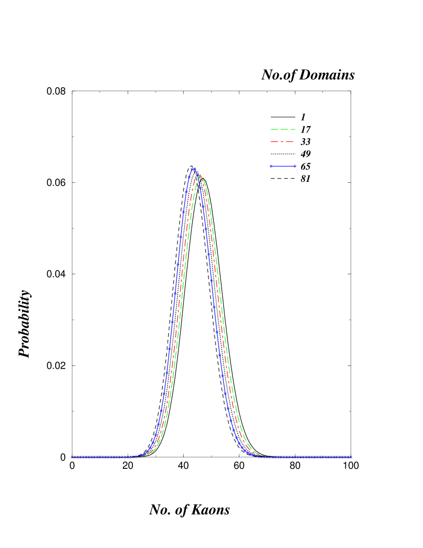
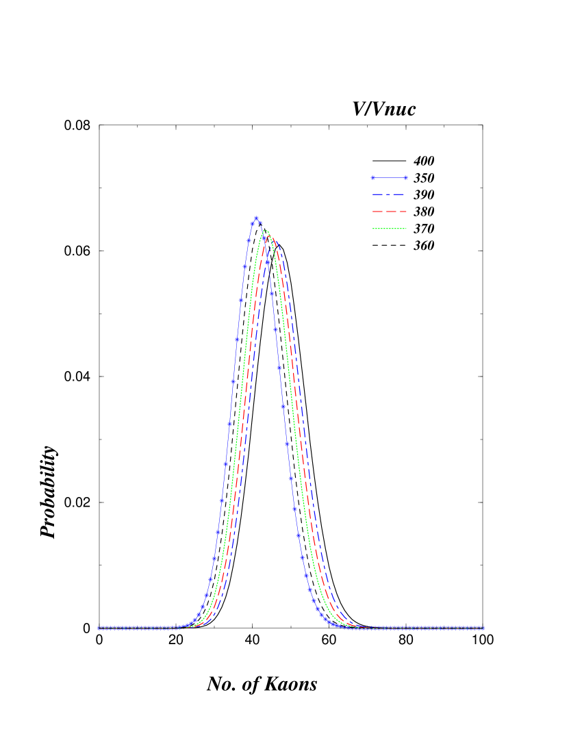
Figure 3: Probability distributions for the production of 0 to 100 Kaons from a maximum total volume $V_{f}=400\,V_{nuc}$ ($V_{nuc}$ is the volume of a nucleon). In the left panel the different distributions represent the different scenarios of the full volume divided into 1 to 81 independent domains. In the right panel the different distributions indicate different cases of total volumes from $400\,V_{nuc}$ to $350\,V_{nuc}$.

Of the variety of strange particles produced in a heavy-ion collision the Kaon is by far the most common and the easiest to identify. We thus compute the probability to obtain $A$ Kaons from the full system that consists of $p$ domains, i.e., $P_{p}^{A}$. The method employed will be almost identical for particles with strangeness -2 ($\Xi$ particles) and -3 ($\Omega$ particles). The $A$ Kaons are indistinguishable bosons: thus the probability to obtain $A$ indistinguishable bosons from $p$ domains may be written schematically as

$$P_{p}^{A}=\frac{D_{p}^{A}}{A!},$$ (20)

where $D_{p}^{A}$ is the probability to obtain $A$ distinguishable Kaons from $p$ partitions. If there are $n_{1}$ Kaons emanating from domain 1, $n_{2}$ from domain 2, etc., then we define the quantity,

$$D_{p}^{A}(n_{1},n_{2}...n_{p})=\frac{A!}{n_{1}!n_{2}!...n_{p}!}D_{1}^{n_{1}}D_{1}^{n_{2}}...D_{1}^{n_{3}}.$$ (21)

Using this we may express the probability to obtain $A$ distinguishable Kaons from $p$ domains as,

$$D_{p}^{A}=\sum_{n_{1},n_{2}...n_{p}|\sum_{i}n_{i}=A}D_{p}^{A}(n_{1},n_{2}...n_{p}).$$

As a result we obtain,

$$P_{p}^{A} = \sum_{n_{1},n_{2},...n_{p}|\sum_{k=1}^{p}n_{k}=A}\frac{D_{1}^{n_{1}}}{n_{1}!}\frac{D_{1}^{n_{2}}}{n_{2}!}...\frac{D_{1}^{n_{p}}}{n_{p}!}$$ (22)

$$= \sum_{n_{1},n_{2},...n_{p}|\sum_{k=1}^{p}n_{k}=A}P_{1}^{n_{1}}P_{1}^{n_{2}}...P_{1}^{n_{p}}.$$

Where $P_{1}^{n_{k}}=\frac{D_{1}^{n_{k}}}{n_{k}!}$ represents the probability to obtain $n_{k}$ indistinguishable Kaons from 1 domain. In Eq. (1) the $S_{k}$ represent the single particle partition functions for particles with strangeness $k$. There are many such particles. The quantity $S_{k}$ is composed of a sum of the single particle partition functions for each of these particles (see Eq. (3)). From Eq. (3) we extract $S(K)$, and define the quantity $\bar{S}_{1}$, as

$$S_{1}=S(K)+S(K^{*})+S(K_{1})+S(\Lambda)+S(\Sigma)+...=S(K)+\bar{S}_{1}.$$

Figure 4: Left panel shows the variation of the mean number of Kaons, probability to produce 20 and 74 Kaons from a volume of size $400\,V_{nuc}$ as the number of domains is increased. The variation with the size of a domain is plotted. All three quantities are normalized to their values for an unpartitioned volume. The right panel plots the variation of the same three quantities from an unpartitioned decreasing volume. All quantities are normalized to their values at $V=400\,V_{nuc}$.

With this, we define a partition function with total strangeness $n$, consisting of only strange particles but not containing any Kaons, as

$$\bar{Z}_{n}=\sum_{n_{1},n_{2},...|\sum kn_{k}=n}\frac{\bar{S}_{1}^{n_{1}}}{n_{1}!}\frac{S_{2}^{n_{2}}}{n_{2}!}\frac{S_{3}^{n_{3}}}{n_{3}!}.$$ (23)

The above partition function, may also be easily evaluated with a similar recursion relation:

$$\bar{Z}_{n}=\frac{1}{n}\Bigg{[}\bar{S}_{1}\bar{Z}_{n-1}+2S_{2}\bar{Z}_{n-2}+3S_{3}\bar{Z}_{n-3}\Bigg{]}.$$

In the above $S_{2}$ and $S_{3}$ remain unaffected. Using the above two equations one may construct the probability $P_{1}^{n}$ of obtaining exactly $n$ Kaons from a single domain, with net strangeness zero. Using Eq. (14), this may be written as,

$$P_{1}^{n}=\frac{Z_{0}}{Z}\frac{S(K)^{n}}{n!}\sum_{N=0}^{\infty}\Bigg{[}\sum_{n_{1},n_{2},n_{3}|\sum in_{i}=N}\frac{\bar{S}_{1}^{n_{1}}}{n_{1}!}\frac{S_{2}^{n_{2}}}{n_{2}!}\frac{S_{3}^{n_{3}}}{n_{3}!}\Bigg{]}Z_{-(N+n)}.$$ (24)

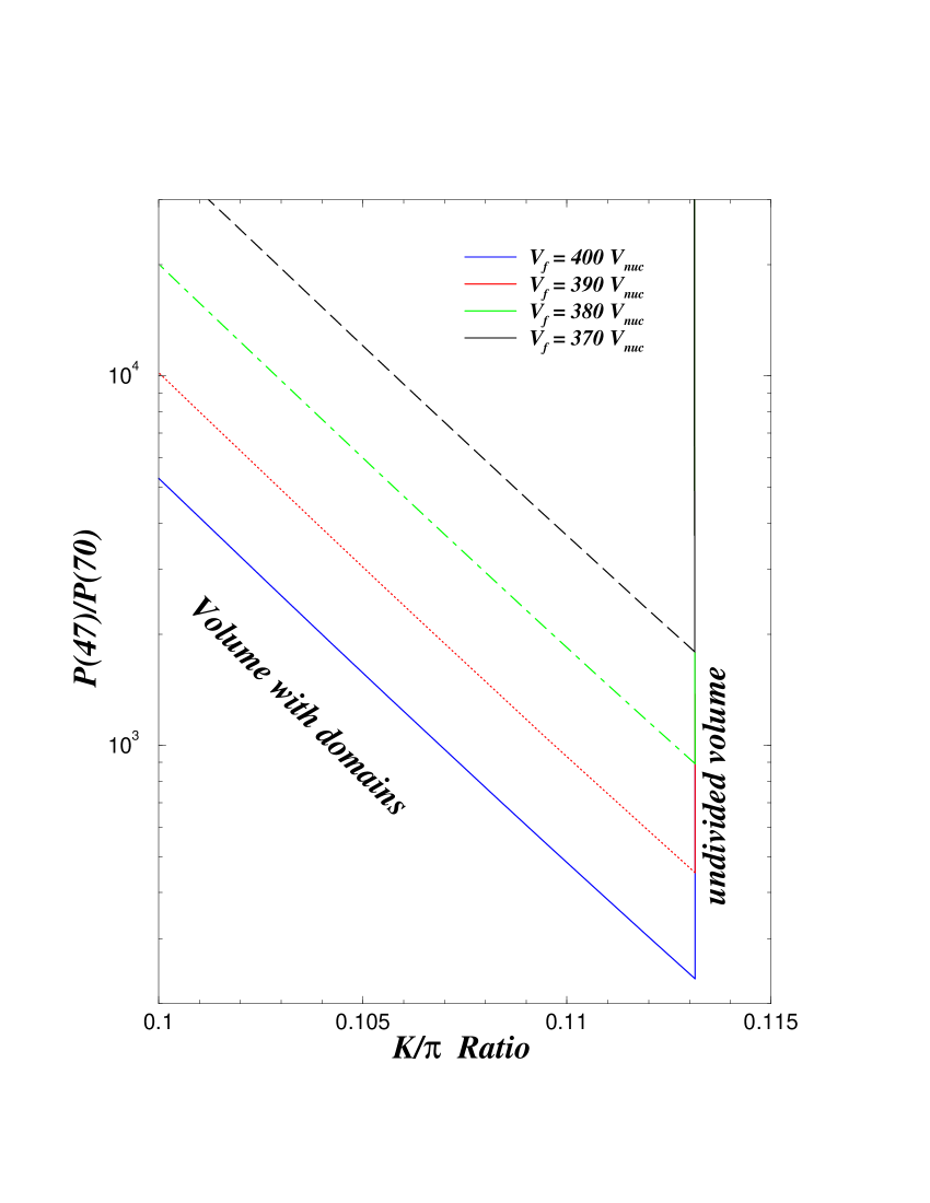
Figure 5: Left panel shows the variation of the the ratio of probabilities $(P(47)/P(70))$ as a function of the mean number of Kaons. The two quantities change as the number of domains is increased, or the total volume is decreased. The right panel shows the variation of the same ratio of probabilities as a function of the $K/\pi$ ratio. The vertical line represents the case of decreasing the total unpartitioned volume. The slanted lines represent the case of increasing the number of domains in a given total volume.

In the above equation, the term in square brackets represents the partition function for a box containing only strange particles, with net strangeness $N$, none of which are Kaons. Obviously, the term in square brackets is simply $\bar{Z}_{N}$. With this we may write down the full probability to obtain $A$ Kaons from the full system with $p$ partitions as

$$P_{p}^{A} = \sum_{n_{1},n_{2},...n_{p}|\sum_{k}n_{k}=A}\left(\frac{Z_{0}}{Z}\right)^{p}\prod_{k=1}^{p}\left(\frac{S(K)^{n_{k}}}{n_{k}!}\sum_{t_{k}=0}^{\infty}\bar{Z}_{t_{k}}Z_{-(t_{k}+n_{k})}\right)$$ (25)

$$= \left(\frac{Z_{0}}{Z}\right)^{p}S(K)^{A}\sum_{n_{1},n_{2},...n_{p}|\sum n_{k}=A}\prod_{k}w_{n_{k}}.$$

In the above equation

$$w_{n_{k}}=\left(\sum_{t_{k}=0}^{\infty}\bar{Z}_{t_{k}}Z_{-(t_{k}+n_{k})}\right)\Bigg{/}n_{k}!$$ (26)

Where $w_{n_{k}}$’s for $0<n_{k}<A$ may be easily calculated using the $\bar{Z}_{t}$ and the $Z_{-t}$’s. The evaluation of the sum with the constraint in Eq. (25) seems to be extremely complicated. However, yet another recursion relation exists which allows this to be computed swiftly. Note that the sum

$$S_{p}^{A}=\sum_{n_{1},n_{2},...n_{p}|\sum n_{k}=A}\prod_{k}w_{n_{k}},$$

requires us to distribute $A$ particles in $p$ distinguishable boxes. If we put $q$ particles in the first box, then we have to distribute $A-q$ particles in $p-1$ boxes. Summing over $q$ gives us the recursion relation,

$$S_{p}^{A}=\sum_{q=0}^{A}w_{q}S_{p-1}^{A-q}.$$ (27)

One may make the simple observation that $S_{1}^{k}=w_{k}$. This along with Eq. (27) allows to calculate the probability $P_{p}^{A}$ recursively. One essentially starts with $S_{1}^{k}$, uses these to build the $S_{2}^{k}$ and so on, until one obtains $S_{p}^{A}$ with the chosen values of $p$ and $A$. A plot of these probabilities is presented in Figs. (3,6,7).

IV Results and discussions

Figure 6: The left panel shows the probability distributions of $\Xi$ particles for a full $V_{f}=400\,V_{nuc}$ and $T=170$ MeV. The volume is divided into various numbers of partitions 1,11,21,31,41,and 51 as shown. The distributions shift slowly towards the left. The mean for each distribution is calculated and is used to compute a Poisson distribution (details in text). The ratio of the calculated probability distributions to the corresponding Poisson distributions is then plotted in the right panel.

We begin the analysis with the kaon distributions (Fig. (3)). In our calculations, the full freeze-out volume $V_{f}$ is taken to be about 400 times the volume of a nucleon. In the left panel of Fig. (3), various cases are presented where this $V_{f}$ is divided into 1,17,33…81 domains. In comparison, the right panel represents the probability distributions for one partition, but for different cases of a decreasing full freeze-out volume. The volumes range from $V_{f}=400\,V_{nuc}$ to $V_{f}=350\,V_{nuc}$. Note that, in the left panel, as the number of domains is increased, the Gaussian like curves slowly shift toward the left. A similar pattern is realised if instead of partitioning the volume, we simply reduced the full volume by 10%, constraining the system to only one domain. Although the probability distributions vary with the partitioning of the system as well as the reduction of the volume, a concise statement about the change, or even the difference between the two cases may not be made from Fig. (3). A clearer picture of the problem may be obtained from Fig. (4): here we plot the mean number of kaons $\langle n_{k}\rangle$ as the number of domains is increased (left panel), and as the the full freeze-out volume is decreased (right panel). For an unpartitioned volume with $V_{f}=400\,V_{nuc}$ the mean $\langle n\rangle\simeq 47$ Kaons. Along with this, we also plot the probability to get $\langle n_{k}\rangle+27$ and $\langle n_{k}\rangle-27$ kaons. These probabilities sample the edges of the probability distributions, which we believe will be most sensitive to a change of the macroscopic conditions. In the following, we will denote these as “edge” probabilities. For an unpartitioned volume with $V_{f}=400\,V_{nuc}$ these “edge” probabilities represent the probabilites to obtain 74 and 20 Kaons. The values of such probabilities are $\sim 10^{-6}$ and are measurable in experiments. One may go even further towards the edges of the distribution to observe a larger effect of partitioning the system, however the values of such probabilities may be too small to be measurable in experiments. In the figure, all values are normalized to the values of the quantities obtained from the unpartitioned maximum volume ($V_{f}=400V_{nuc}$). Note that the mean hardly changes as we increase the number of domains, or reduce the volume. The “edge” probabilities however display substantial variation. In a real heavy-ion collision, one can never determine the volume to a great degree of accuracy (in the case of flow, the very meaning of the volume becomes complicated). Hence, the similarity of the two plots makes it difficult to distinguish between the two cases. If only the kaon probability distributions were measured, sole observation of these would not allow one to distinguish between these two cases. Measurements of other observables, not constrained by strangeness conservation (such as pion yields), will have to be invoked.

Even though the “edge” probabilities in the left and right panels of Fig. (4) look substantially different, one cannot simply superpose the two figures to make a comparison, the $x$-axis in both graphs represent very different quantities. One may use a limiting procedure by calculating the absolute number of particles not constrained by conservation laws, such as pions. These are sensitive to the total volume and can be used to set constraints on the total volume. This limits the range of the $x-$axis of the right panel of Fig. (4). Such a constraint will set limits on the maximum spread between the two “edge” probabilities. If the spread between the “edge” probabilities in the left panel went beyond the limits set by the right panel, then one would be lead to the conclusion that a large thermalized system was not formed. Thus, to determine the amount of partitioning of the total volume, one would need to determine the pion or proton yields with an error somewhat smaller than the range of the $x$-axis of Fig.(4). Thus, discering the degree of thermalization will require accurate experimental results.

Figure 7: Same as Fig. (6) but for the $\Omega$ particles.

As mentioned before, a change in the total volume would lead to a noticeable change in the pion number. The kaon-to-pion ratio, however, would remain almost constant in the case of a single domain, as both are proportional to the volume. The behavior of this ratio versus the volume, for a single domain, is plotted in Fig. (2). In Fig. (5) (right panel), we plot a ratio of probabilities versus the $K/\pi$ ratio from both scenarios. The choice of which two probabilities to use is arbitrary. We chose the numerator near the peak of the distribution $(P(47))$, while the denominator is chosen near the edge $(P(70))$. In the following, this will be denoted as the “peak-edge” ratio. The motivation behind this choice is that as the probability distributions (in Fig. (3)) shift towards the left, the value near the peak changes marginally in comparison to the value at the edge, which drops rapidly. Experimentally, this will correspond to the case where the temperature $T$ has been measured from other ratios. This temperature $T$ is then used to plot the curves in Fig. (5). The vertical line represents the case of particle production from an unpartitioned volume. The $K/\pi$ ratio is almost a constant as expected. The “peak-edge” ratio simply grows as the volume is reduced. The slanted set of lines represents the case for multiple domains. The $K/\pi$ ratio drops as the number of domains increases. As the total volume is unchanged, the number of pions remains fixed. The different lines represent different cases where we have considered smaller freeze-out volumes $V_{f}$. The cases plotted are for $V_{f}=400,\,390,\,380,\,370\,V_{nuc}$. Thus, the triangular region represents the “allowed region” where an experimental point may lie if such an observation were made. The location of the vertical line of the region depends solely on the temperature. The location of the actual experimental point allows one to decipher not only the total volume which contributes to the production of particles but also the size of the domain over which strangeness is conserved. However, as before, we note that, even though the “peak-edge” ratio varies over many orders of magnitude; the $K/\pi$ ratio shows only a 15 % variation. Thus, both the $K/\pi$ ratio and $T$ have to be determined with an error much less than 15 %. This reinstates our earlier result that accurate experimental results are required to quantitatively describe the degree of thermalization.

The importance of an accurate measurement of the pion yield may be further underlined if we plot the “peak-edge” ratio versus only the kaon yield, this is done in the left panel of Fig. (5). The solid line represents the variation of the “peak-edge” ratio of probabilities with the mean number of Kaons emanating from multiple domains in a full volume of $400\,V_{nuc}$. The dot-dashed line represents the same comparison but for a total volume descending from a maximum value of $400\,V_{nuc}$. Note that both curves lie almost on top of one another. The “peak-edge” ratio drops slightly more sharply for the partitioned case. The main reason for the two plots being similar is, not an ill choice of the probability ratio, but rather, the mean number of kaons, which varies almost linearly with change in volume for volumes in the range of $350-400\,V_{nuc}$. This allows the kaon number to change by almost the same range in both plots. If we were to proceed to a much smaller number of kaons the two graphs would then separate from each other. This demonstrates, yet again, the similarity of the probability distributions in Fig. (3).

The primary reason for the requirement of accurate experimental data is the low sensitivity of the kaon yields to the domain volume. At temperatures in the vicinity of 170MeV a large number of kaons ($\sim 50$) are produced. This causes the kaon yields to approach the grand canonical limit, in other words the kaons yields do not experience sufficient canonical suppression. A similar trend has recently been observed in a partonic scenario at higher temperature pra03 , where very small volumes are required to observe canonical suppression. Naïvely, one would expect multiple strange particles to be subject to greater canonical strangeness conservation. We present the probability distributions for particles of strangeness -2 (i.e., $\Xi$ particles) and strangeness -3 (i.e., $\Omega$ particles). These are plotted in the left panels of Figs. (6,7). We note that, as expected, the difference between the distributions is more pronounced for the $\Xi$ particles, and even more for the $\Omega$ particles, as the number of domains is increased. The $\Xi$ distributions are peaked near 1 to 3 particles. The mean number is about 2 $\Xi$ particles. The $\Omega$ distributions are peaked at zero and the mean number is a fraction. We note that there is an order of magnitude difference between the probability to obtain 10 $\Xi$ particles from one domain compared to that from 51 domains. The same is true for the probability to obtain 5 $\Omega$ particles. The minimum probabilities in this region are $\sim 10^{-6}$ and hence, are in principle measurable at RHIC. It should be pointed out that, the effect of canonical strangeness conservation, for cases where we have greater than 20 partitions (or domain volumes smaller than $20\,V_{nuc}$), may be deduced by an accurate determination of the mean numbers of kaon, $\Xi$ and $\Omega$ particles (see Fig. (8)). From Fig. (8) we note that a determination of the mean number of $\Omega$ particles with an accuracy of 5% will allow one to estimate the domain volume up to a volume of $V=20\,V_{nuc}$ (this is for the case of full freeze-out volume $V_{f}=400\,V_{nuc}$ and a $T=170$ MeV ). For domain volumes greater than this, one will need to determine the mean numbers with very high accuracy (errors $\sim 1$ %). Alternatively, one may determine the probability to obtain 5 $\Omega$ particles with an accuracy of 20%, or the probability to obtain 10 $\Omega$ particles with an accuracy of 50%. Similar error bars may also be deduced for the cascades. Which observable is better suited to the determination of the domain size, now becomes a question of experiment. The behaviour of experimental data on the mean numbers of strange particles hoh03 (see also the canonical model analysis in Ref. ker02 ) indicates that the number of partitions, in central collisions, is in the range from 1 to 20 i.e., the region in Fig. (8) where the mean values reach a plateau. As a result of this, determination of the amount of partitioning of the system (i.e., resolving the domain size between $V=20\,V_{nuc}$ to domain size of the order of the freeze-out volume $V=V_{f}$) will require very accurate measurements of the means or the probability distributions.

In the above discussion, we have demonstrated that the “edges” of the probability distributions for $\Xi$ particles and $\Omega$ particles are sensitive to the partitioning of the system (we also pointed out that the mean yields also shift by about 20% as we go from 1 to 51 partitions). This variation in the probability distributions is an indication that these particles are experiencing canonical suppression. Recall the situation of pion production which is insensitive to the partitioning of the system, the pion yields are calculated in the grand canonical ensemble. The probability distributions from such an ensemble are Poissonian. A more quantitative measure of the departure of the $\Xi$ and $\Omega$ production from the grand canonical limit may be obtained from the ratio of the probability distributions to the corresponding Poisson distributions. Using the mean $\langle n\rangle$ we may construct a Poisson distribution to obtain $n$ $\Xi$ particles from $p$ domains as,

$$P^{n}_{p}=\frac{\langle n\rangle^{n}}{n!}{e^{-\langle n\rangle}}.$$

The ratio of the actual, calculated, probability distribution to the Poisson probability distribution is plotted in the right panel of Fig. (6) for varying number of domains as indicated. We note that the probability distributions closely resemble a Poisson distribution up to the probability to obtain about eight $\Xi$ particles. Beyond this the distributions begin to deviate from a Poisson distribution. The same ratio is also plotted for the $\Omega$ particles in Fig. (7). The $\Omega$ distribution remains Poissonian up to five $\Omega$ particles.

An interesting pattern that may be noted both for the $\Xi$ and $\Omega$ distributions is that the probability distributions approach the Poisson distribution as the number of domains is increased compared to the number of particles (see the right panels of Figs. (6,7)). This effect is much more pronounced in the case of the $\Omega$ distributions. This may be understood as follows: in the case of a single, small domain, the $\Omega$ probability distribution achieves an almost binary configuration. The probability $b$ to produce zero $\Omega$ particles is large (i.e., $b\rightarrow 1$), followed by a small probability $a$ to produce one $\Omega$ particle (i.e., $a\rightarrow 0$). The probability to produce multiple $\Omega$ particles is very small and hence may be ignored (i.e., $a+b=1$). If there are $p$ domains, the probability to obtain $n$ $\Omega$ particles is given by the simple binary distribution,

$$P_{p}^{n}=\frac{p!}{n!(p-n)!}a^{n}b^{p-n}.$$ (28)

As $p$ becomes much larger than $n$, the binary distribution turns into the Poisson distribution. This is why the ratio of probabilities in Figs. (6,7) (right panels) begins to deviate from 1 as we go to higher and higher numbers of particles. This corresponds to increasing $n$. Increasing the number of domains (keeping the volume of each domain constant) corresponds to increasing $p$. If instead, the total volume is held fixed and the number of domains is increased, then aside from the increase in $p$, the production of $\Omega$ particles from each domain approaches the binary limit. As a result of these two effects, increasing the number of domains drives the probability distribution function towards the Poisson value. Similar effects in moderation may be ascribed to the $\Xi$ probability distribution functions. Thus, when the number of domains is large compared to the number of particles produced, one obtains a Poisson like probability.

Figure 8: Mean and Variance for Kaons, $\Xi$ and $\Omega$ particles for a $T=170$MeV, and a total $V=400\,V_{nucleon}$. The number of domains varies from 1 to 51.

As pointed out in the previous paragraph, $\Omega$ production from a single, small domain has a binary configuration, i.e., a very narrow distribution ($P(n)\neq 0$ only for $n=0,\,1$ ). The distribution from many such domains (see left panel of Fig. (6)), is necessarily broader due to fluctuations. However, even for the case of no partitioning, the probability to produce two $\Omega$ particles from the full freeze-out volume is suppressed by a factor of three compared to that for a single $\Omega$, i.e., the distributions are still rather narrow (see left panel of Fig. (7)). An amusing consequence of this is that the variance of the $\Omega$ distribution is equal to its mean. The variance is defined as

$$\sigma=\langle n^{2}\rangle-\langle n\rangle^{2}=\sum_{n}n^{2}P(n)-\left(\sum_{n}nP(n)\right)^{2},$$

where $P(n)$ is the probability to obtain $n$ $\Omega$ particles. This equality would indicate that the $\Omega$ yields are tending towards the grand canonical limit, whereas the situation is quite the opposite. This is illustrated in Fig. (8), here we plot the mean and variance of the the Kaons, $\Xi$ and $\Omega$ particles. For a grand canonical ensemble (no suppression), the distribution is Poissonian. As a result, the variance equals the mean. As we note from Fig. (8), the $\Omega$ particles seem to exhibit a Poissonian variance, whereas the $\Xi$ particles deviate slightly from this limit. The Kaons display a noticeably different variance from the Poissonian value. As pointed out previously, the reason behind this rather contradictory result is the fact that the $\Xi$ and $\Omega$ distributions descend rapidly from their peak values (see left panels of Figs. (6,7)). The decent is much more mild for the kaons (see left panel of Fig. (3)). All three types of particle distributions show a Poissonian behavior near the “peak” of the distribution, deviating from such behavior as one proceeds to the “edges” of the distribution. The Kaon distribution resembles a Poisson distribution over a much wider range than the $\Xi$ or $\Omega$ distributions (see Fig. (9)). While the $\Xi$ and $\Omega$ distributions predominantly sample the region in the vicinity of the “peak”, the variance of the kaons receives support from a wider region. This causes the $\Xi$ and $\Omega$ variance to approach that of a Poisson distribution, while the kaon variance falls below this limit. Hence, the appearance of a Poisson like variance is not indicative of a lack of canonical suppression, and vice-versa.

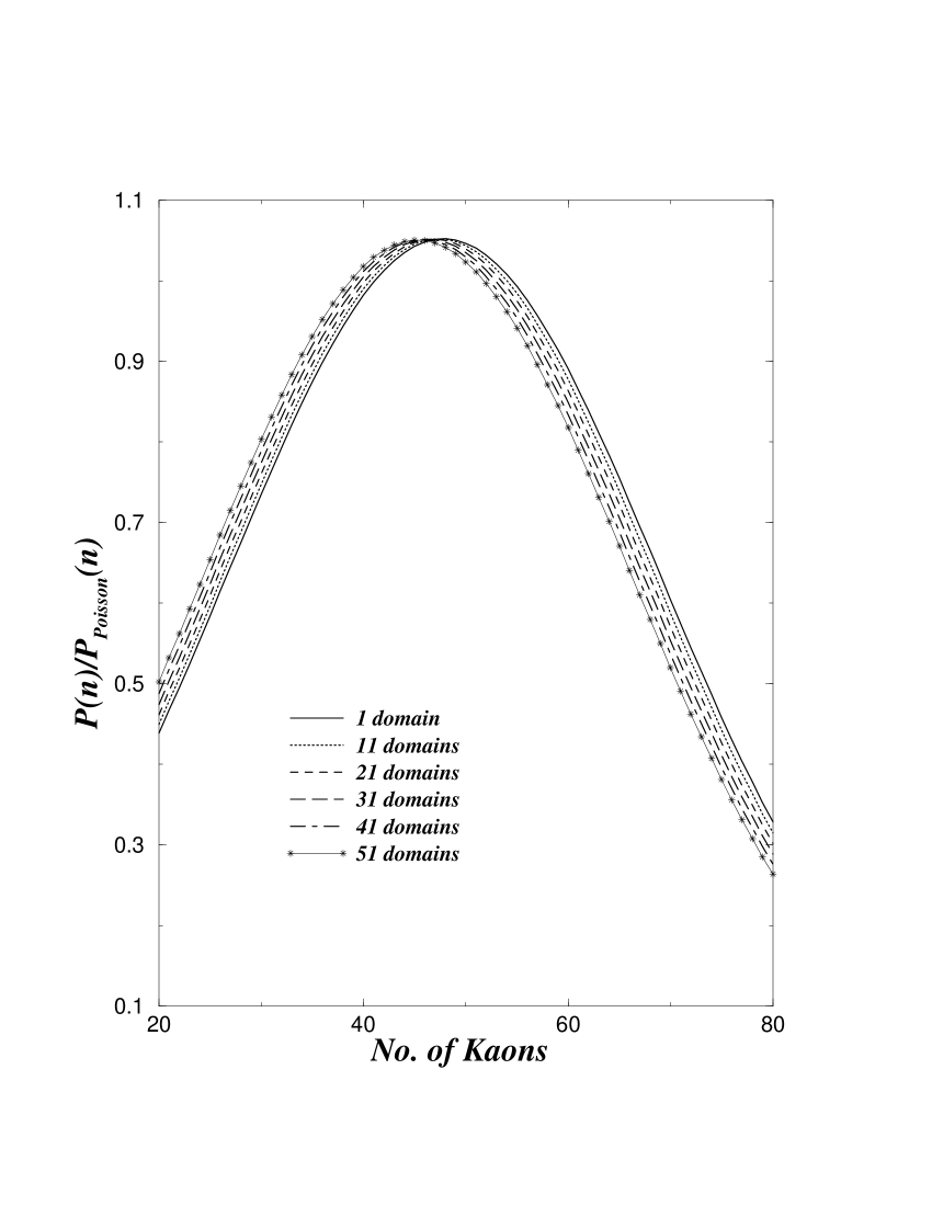
Figure 9: Ratio of the calculated probability distribution of the Kaons to the Poisson distribution. Same as right panel of Fig. (6).

A study of Fig. (8) indicates that the Kaon variance does not tend towards its mean, even as the volume is increased. This may be understood by a simple analytical argument. Imagine a large freeze-out volume ($V_{f}>400\,V_{nuc}$) at a sufficiently high temperature ($T\sim 170$ MeV). If the only particles carrying a conserved strangeness quantum number are kaons and anti-kaons, one would expect a large number of these to be produced ( $\langle N_{K}\rangle=\langle N_{\bar{K}}\rangle\sim 100$). In fact, the mean number of kaons $\langle N_{K}\rangle$, anti-kaons $\langle N_{\bar{K}}\rangle$ and the total, mean, number of strangeness carrying particles $\langle N\rangle$ can now be estimated by a grand canonical ensemble. Strangeness conservation, however, is imposed by the following relation

$$N_{K}+N_{\bar{K}} = N$$

$$N_{K}-N_{\bar{K}} = 0.$$ (29)

We may square the above equations, take the mean and sum them to obtain,

$$2\langle N_{K}^{2}\rangle+2\langle N_{\bar{K}}^{2}\rangle=\langle N^{2}\rangle.$$ (30)

We may also take the mean and then square and sum to obtain,

$$2\langle N_{K}\rangle^{2}+2\langle N_{\bar{K}}\rangle^{2}=\langle N\rangle^{2}.$$ (31)

We may now subtract Eq. (31) from Eq. (30) to obtain the variance. As the total number of particles carrying strangeness, $N$, is not a conserved quantity, its distribution may be estimated accurately by a grand canonical ensemble (i.e., a Poisson distribution). Hence, the variance of $N$ is equal to its mean, i.e.,

$$\sigma_{N}=\langle N\rangle=\langle N_{K}\rangle+\langle N_{\bar{K}}\rangle.$$ (32)

From the second line of Eq. (29) we obtain

$$\langle N_{K}\rangle = \langle N_{\bar{K}}\rangle$$

$$\sigma_{N_{K}} = \sigma_{N_{\bar{K}}}.$$ (33)

From Eqs. (30-33) we obtain,

$$\sigma_{N_{K}}=\frac{N_{K}}{2}.$$ (34)

Thus, the kaon variance is equal to half of that of a Poisson distribution, even for a large system. The presence of particles other than kaons in the partition sums calculated previously allow for more fluctuation of the conserved strangeness among different strangeness carriers. This increases the variance from $\frac{N_{K}}{2}$ to the value plotted in Fig. (8).

It should be pointed out that measurements of the variance of the $K/\pi$ ratio at the SPS indicate a Poisson value, at forward rapidities afa01 (central region in fixed target experiments). This has been shown to be consistent with a Poisson variance for the kaon number jeo99 . This is in contradistinction with Fig. (8). This indicates that there is a contamination of the kaon number from neighbouring rapidity intervals. This contamination is essentially random from event to event and thus leads to an increased fluctuation of the kaon numbers. This will cause the variance to increase and lead it to becoming Poissonian. If instead, it were possible to measure the kaon yields over a larger acceptance, the percentage of random fluctuation in the kaon variance would reduce and one should begin to approach the value in Fig. (8). This serves as an important test to ensure the observation of strangeness production from a closed volume; i.e., a region whose strange yields are not influenced (event by event) by strange yields from neighbouring regions.

V Summary and Conclusions

The principal question addressed in this article has been the degree of thermalization achieved in heavy-ion collisions, and whether this question may be answered within the framework of statistical models (i.e., without invoking hard or penetrating probes). We began with the understanding that complete equilibrium and simple superposition of proton-proton collisions are extreme possibilities. We quantified the degree of thermalization as the size of the domain within which thermalization is achieved, independent of many other such domains which may be formed. The domain was defined as the region over which chemical equilibrium (in particular strangeness chemical equilibrium) was achieved. Given the fact that chemical equilibrium is achieved at a slower rate than kinetic equilibrium, estimating the size of such a domain would set a lower bound on the size of the kinetically equilibrated region.

We further restricted the definition of the domain as the volume within which strangeness in strictly conserved. A more complete calculation with baryon number also strictly conserved may also be performed; this has been left for a future effort maj03 . Mean baryon number is set by means of a chemical potential. In this preliminary effort, a study of the effect of varying chemical potential was not performed; $\mu$ was set to zero throughout. The full freeze-out volume was postulated to consist of many such domains. Throughout the calculation, the full freeze-out volume $V_{f}$ was set to $400\,V_{nucleon}$ and the temperature to $170$ MeV. These chosen values of the thermodynamic parameters $T,\,V_{f},\,\mu$ are approximately in agreement with collisions at RHIC. As a result, the domain size $V$ became $V_{f}/p$, where $p$ is the number of domains. The estimation of the domain size was performed by noting the behavior of the total probability distributions of various strange particles as a function of $p$. These results are essentially contained in Figs. (3-8). These probability distributions are, in principle, measurable in heavy-ion collisions.

In the calculation of all the above quantities (e.g., mean, variance, probability distributions etc.), we have made express use of the recursion relation technique cha95 ; das98 ; das99 , grafted from intermediate energy heavy-ion physics. This technique greatly simplifies numerical calculations in the canonical ensemble with exact conservation conditions. Two different sets of recursion relations have been devised: the first one calculates the partition functions, and its derivatives in a given domain (Eqs. (11,17,19)), while the second convolutes the probability distributions from different domains (Eq. (27)). Without the use of recursion relation techniques, such probability distribution calculations may become prohibitively difficult.

It is clear from the behavior of the mean numbers of Kaons, $\Xi$ and $\Omega$ particles in Fig. (8) and the numbers seen in experiments hoh03 , that domain sizes of the order of a nucleon volume are eliminated. The question reduces to resolving the domain size between $V=20\,V_{nuc}$ ($p=20$) to domain size of the order of the freeze-out volume $V=V_{f}$. A definite result for $V$ will involve an accurate determination of the probability distributions of the Kaons, $\Xi$ and $\Omega$ particles, and comparison with Figs. (3-7). Alternatively, one may determine the yields with much greater accuracy than presently imposed in heavy ion collisions and compare with Fig. (8). Such a measurement will set a lower bound on the size of the region over which thermal equilibrium has been established. We also pointed out that measurements of two particle correlations, such as the variance, may lead to incorrect conclusions regarding the amount of canonical suppression faced by different strangeness carriers.

As a corollary, we note that partitioning the system introduces a new parameter $p$, which essentially changes the yields of strange particles keeping the pion yields fixed. Hence this provides a natural formalism to understand the difference between the $K/\pi$ ratio in central collisions of small systems compared to non-central collisions of large nuclei, with the same $N_{part}$ in both cases (see e.g., Ref. kam03 ). Fitting the experimental points involves introducing various refinements (e.g., Baryon number conservation, temperature and volume fluctuations among domains etc.) to the rather simple model presented above. These and other considerations will be addressed in a future effort maj03 .

VI Acknowledgment

The authors wish to thank X. N. Wang for helpful discussions. This work was supported in part by the Natural Sciences and Engineering Research Council of Canada and by the Director, Office of Science, Office of High Energy and Nuclear Physics, Division of Nuclear Physics, and by the Office of Basic Energy Sciences, Division of Nuclear Sciences, of the U.S. Department of Energy under Contract No. DE-AC03-76SF00098.

References

- (1) J. C. Collins and M. J. Perry, Phys. Rev. Lett. 34, 1353 (1975).
- (2) E. Shuryak, Phys. Rep. 80, 71 (1980).
- (3) R. C. Hwa, and X. N. Wang, Phys. Rev. D. 42, 1459 (1990).
- (4) P. Braun-Munzinger, I. Heppe, and J. Stachel, Phys. Lett. B465, 15 (1999).
- (5) P. Braun-Munzinger, D. Magestro, K. Redlich, and J. Stachel, Phys. Lett. B518, 41 (2001).
- (6) J. Rafelski, J. Letessier, and G. Torrieri, Phys. Rev. C. 64, 054907 (2001); Erratum-ibid. C. 65, 069902 (2002).
- (7) D. Zschiesche, S. Schramm, J. Schaffner-Bielich, H. Stocker, and W. Greiner, Phys. Lett. B547, 7 (2002).
- (8) W. Broniowski, and W. Florkowski, Phys. Rev. Lett. 87, 272302 (2001).
- (9) W. Broniowski, and W. Florkowski, Phys. Rev. C. 65, 064905 (2002).
- (10) R.J. Fries, B. Muller, C. Nonaka, and S.A. Bass, nucl-th/0301087.
- (11) V. Koch, Proc. Quark Matter 02, Nucl. Phys. A715, 108c (2003).
- (12) F. Becattini, and U. Heinz, Z. Phys. C. 76, 269 (1997).
- (13) S. Jeon, and V. Koch, Phys. Rev. Lett. 85, 2076 (2000).
- (14) M. Bleicher, S. Jeon, and V. Koch, Phys. Rev. C. 62, 061902 (2000).
- (15) C. Adler, et. al., Phys. Rev. Lett. 89, 202301 (2002).
- (16) J. Adams, et. al., nucl-ex/0211024.
- (17) R. Hagedorn, Supp. Nuovo Cimento 6, 31 (1968).
- (18) F. Reif, Statistical and Thermal Physics, McGraw-Hill, Singapore (1985).
- (19) J. Cleymans, K. Redlich, and E. Suhonen, Z. Phys. C. 51, 137 (1991).
- (20) S. Hamieh, K. Redlich, and A. Tounsi Phys. Lett. B486, 61 (2000).
- (21) K. C. Chase, and A. Z. Mekjian Phys. Rev. Lett. 75, 4732 (1995).
- (22) S. Das Gupta and A. Z. Mekjian, Phys. Rev. C. 57, 1361 (1998).
- (23) S. Das Gupta, A. Majumder, S. Pratt and A. Z. Mekjian, nucl-th/9903007.
- (24) A. Majumder, in preparation.
- (25) C. Hohne et. al., Proc. Quark Matter 02, Nucl. Phys. A715, 474c (2003).
- (26) A. Keränen, and F. Becattini, Phys. Rev. C. 65, 044901 (2002).
- (27) S. V. Afanasiev, et. al., Phys. Rev. Lett. 86, 1965 (2001).
- (28) S. Jeon, and V. Koch, Phys. Rev. Lett. 83, 5435 (1999).
- (29) S. Pratt, and J. Ruppert, nucl-th/0303043.
- (30) B. Kampfer, J. Cleymans, P. Steinberg, and S. Wheaton, Proc. 19th Winter Workshop on Nuclear Dynamics, 2003, hep-ph/0304269.