Critical Points in Nuclei and
Interacting Boson Model Intrinsic States

Abstract

We consider properties of critical points in the interacting boson model, corresponding to flat-bottomed potentials as encountered in a second-order phase transition between spherical and deformed $\gamma$-unstable nuclei. We show that intrinsic states with an effective $\beta$-deformation reproduce the dynamics of the underlying non-rigid shapes. The effective deformation can be determined from the the global minimum of the energy surface after projection onto the appropriate symmetry. States of fixed $N$ and good $O(5)$ symmetry projected from these intrinsic states provide good analytic estimates to the exact eigenstates, energies and quadrupole transition rates at the critical point.

“During these moments of abstraction he seemed more intimately absolved, in the sense of being linked anew with the universe.

Giuseppe de Lampedusa, “The Leopard”

1 Introduction

In the days that one of us (JNG) was a graduate student, group theory was considered almost a dirty word in the nuclear physics community even though Wigner had introduced spin-isospin symmetry (SU(4)), Elliott had exploited the symmetry of the harmonic oscillator to link collective motion and the shell model (SU(3)) and the symmetry of the hadrons had been discovered (SU(3) again). Francesco Iachello changed that attitude and brought group theory front and center in nuclear physics and in other fields of physics.

Franco Iachello is a descendant of a noble Sicilian family similar to that portrayed in Giuseppe de Lampedusa’s classic Italian novel, “The Leopard”. Set in Sicily in 1860 at the time of the campaign for the unification of Italy, the hero, the Prince, struggles with how to keep the old while embracing the new. The Prince often took solace from the turmoil of the real world by studying astronomy and mathematics much the same as Franco has by his significant contributions to physics and group theory.

2 Critical Points in the Geometric Collective Model

Recently Franco has been studying two critical points associated with shape phase transitions in nuclei within the geometric framework of the collective model for infinite square well potentials [1, 2] . This model involves a Bohr Hamiltonian which describes the dynamics of a macroscopic quadrupole shape via a differential equation in the intrinsic quadrupole shape variables beta and gamma. In the current contribution we shall discuss the critical point (CP) for a second order shape phase transition between spherical and deformed $\gamma$-unstable nuclei, which Franco called E(5) [1]. An empirical example of such a critical point has been found in ¹³⁴Ba [3, 4] and possibly in ¹⁰⁴Ru [5], ¹⁰²Pd [6] and ¹⁰⁸Pd [7].

Table 1: Excitation energies (normalized to the energy of the first excited state) and B(E2) values (in units of $B(E2;\,2^{+}_{1,1}\rightarrow 0^{+}_{1,0})=1$) for the E(5) critical point [1], for several N=5 calculations and for the experimental data of ¹³⁴Ba [15]. The finite-N calculations involve the exact diagonalization of the critical IBM Hamiltonian ($H_{cri}$) [Eq. (19)], $\tau$-projected states for $H_{cri}$ [Eqs. (9),(12) with $y=0.314$], the $U(5)$ limit [$\epsilon\,n_{d}$] and the $O(6)$ limit [$(A/4)(N-\sigma)(N+\sigma+4)+B\tau(\tau+3)$].

	E(5)	exact	$\tau$-projection	U(5)	O(6)	134Ba
		N=5	N=5	N=5	N=5	exp
$E(0^{+}_{1,0})$	0	0	0	0	0	0
$E(2^{+}_{1,1})$	1	1	1	1	1	1
$E(L^{+}_{1,2})$	2.20	2.195	2.19	2	2.5	2.32
$E(L^{+}_{1,3})$	3.59	3.55	3.535	3	4.5	3.66
$E(0^{+}_{2,0})$	3.03	3.68	3.71	2	$1.5{A\over B}$	3.57
$B(E2;\,4^{+}_{1,2}\rightarrow 2^{+}_{1,1})$	1.68	1.38	1.35	1.6	1.27	1.56(18)
$B(E2;\,6^{+}_{1,3}\rightarrow 4^{+}_{1,2})$	2.21	1.40	1.38	1.8	1.22
$B(E2;\,0^{+}_{2,0}\rightarrow 2^{+}_{1,1})$	0.86	0.51	0.43	1.6	0	0.42(12)

In the geometric approach the E(5) eigenfunctions [1] are proportional to Bessel functions of order $\tau+{3\over 2}$ and the corresponding eigenvalues are proportional to $(x_{\xi,\tau})^{2}$. Hamiltonians that are $\gamma$- unstable have an $O(5)$ symmetry and $\tau$ is the $O(5)$ quantum number. Furthermore

$x_{\xi,\tau}$ is the $\xi$-th root of these Bessel functions. A portion of an E(5)-like spectrum is shown in Fig. 1. It consists of states, $L^{+}_{\xi,\tau}$, arranged in major families labeled by $\xi=1,2,\ldots$ and $O(5)$ $\tau$-multiplets ($\tau=0,1,\ldots$) within each family. The angular momenta $L$ for each $\tau$-multiplet are obtained by the usual $O(5)\supset O(3)$ reduction [8]. The E(5) CP leads to analytic parameter-free predictions for energy ratios and $B(E2)$ ratios which persist when carried over to a finite-depth potential [9]. As seen in Table 1, the E(5) predicted values are in-between the values expected of a spherical vibrator [$U(5)$] and a deformed $\gamma$-unstable rotor [$O(6)$].

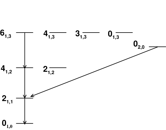
Figure 1: An E(5)-like spectrum of states labeled by $L_{\xi,\tau}$. Shown are the transitions whose B(E2) values are given in Eq. (12). The E2 rates for other $\Delta\tau=1$ transitions (not shown) are governed by O(5) symmetry. Specifically, $B(E2;\,L^{+}_{1,2}\longrightarrow 2^{+}_{1,1})$ for $L=4,2$ are in the ratio $1:1$ respectively, $B(E2;\,L^{+}_{1,3}\longrightarrow 4^{+}_{1,2})$ for $L=6,4,3$ and $B(E2;\,L^{+}_{1,3}\longrightarrow 2^{+}_{1,2})$ for $L=4,3,0$ are in the ratios $1:10/21:2/7:11/21:5/7:1$, respectively. Taken from ref.[13].

3 Wave Function Ansatz for the $\gamma$-Unstable Limit of the Interacting Boson Model

The Interacting Boson Model [10] (IBM) was one of the great achievements of Akito Arima and Franco Iachello. This model describes low-lying quadrupole collective states in nuclei in terms of a system of $N$ monopole ($s$) and quadrupole ($d$) bosons representing valence nucleon pairs. The IBM Hamiltonian relevant to the critical point of the phase transition between spherical and $\gamma$-unstable deformed nuclei has $O(5)$ symmetry [11]. Its energy surface, obtained by the method of coherent states [11, 12], is $\gamma$-independent and exhibits a flat-bottomed behavior in $\beta$ which resembles the infinite square-well potential used to derive the E(5) CP in the geometric approach [1]. Calculations with finite $N$ values ($N$=5 for ¹³⁴Ba) have found that this critical IBM Hamiltonian can replicate numerically the E(5) CP and its analytic predictions [3, 5, 6, 7]. In the present contribution, based on recent work [13], we examine the properties and conditions that enable features of E(5) CP to occur in a finite system described by the interacting boson model. For that purpose we propose wave functions of a particular analytic form, which can simulate accurately the exact IBM eigenstates at the critical point. These wave functions with fixed $N$ and good $O(5)$ symmetry are used to derive accurate estimates for energies and quadrupole rates at the critical point without invoking large-$N$ approximations. The proposed wave functions can be obtained by projection from intrinsic states with an effective $\beta$-deformation.

In the IBM, the $\gamma$-unstable transition region is modeled by the Hamiltonian

$$H = \epsilon\,\hat{n}_{d}+{1\over 4}A\,\left[\,d^{\dagger}\cdot d^{\dagger}-(s^{\dagger})^{2}\,\right]\left[\,H.c.\,\right]$$ (1)

with $\epsilon$ and $A$ positive parameters. Here $\hat{n}_{d}$ is the $d$-boson number operator, $H.c.$ stands for Hermitian conjugate and the dot implies a scalar product. In the $U(5)$ limit ($A=0$), the spectrum of $H$ is harmonic, $\epsilon\,n_{d}$, with $n_{d}=0,1,2\ldots N$. The eigenstates are classified according to the chain $U(6)\supset U(5)\supset O(5)\supset O(3)$ with quantum numbers $|\,N,n_{d},\tau,L\rangle$ (for $\tau\geq 6$ an additional multiplicity index is required for complete classification). These states can be organized into sets characterized by $n_{d}=\tau+2k$. States in the lowest-energy set ($k=0$) satisfy

$$P_{0}\,|\,N,n_{d}=\tau,\tau,L\rangle=0$$

$$P_{0}^{\dagger}=d^{\dagger}\cdot d^{\dagger}~{}.$$ (2)

Other sets ($k>0$) are generated by $|\,N,n_{d},\tau,L\rangle\propto(P^{\dagger}_{0})^{k}|\,N-2k,n_{d}=\tau,\tau,L\rangle$. In the $O(6)$ limit ($\epsilon=0$), the spectrum is ${1\over 4}A(N-\sigma)(N+\sigma+4)$ with $\sigma=N,N-2,N-4,\ldots 0\;{\rm or}\;1$. The eigenstates are classified according to the chain $U(6)\supset O(6)\supset O(5)\supset O(3)$ with quantum numbers $|\,N,\sigma,\tau,L\rangle$. The ground band has $\sigma=N$ and its members satisfy

$$P_{1}\,|\,N,\sigma=N,\tau,L\rangle=0$$

$$P^{\dagger}_{1}=[\,d^{\dagger}\cdot d^{\dagger}-\,(s^{\dagger})^{2}\,]~{}.$$ (3)

The remaining bands with $\sigma=N-2k$ are generated by $|\,N,\sigma,\tau,L\rangle\propto(P^{\dagger}_{1}))^{k}\,|\,N-2k,\sigma,\tau,L\rangle.$ These results suggest that in-between the $U(5)$ and $O(6)$ limits, we consider a ground band ($\xi=1$) for the Hamiltonian (1) determined by the condition

$$P_{y}\,|\,\xi=1;y,N,\tau,L\rangle=0~{},$$

$$P^{\dagger}_{y}=\left[\,d^{\dagger}\cdot d^{\dagger}-y\,(s^{\dagger})^{2}\,\right].$$ (4)

In the $U(5)$ basis these states are

$$|\,\xi=1;y,N,\tau,L\rangle = \sum_{n_{d}}{1\over 2}\left[1+(-1)^{n_{d}-\tau}\right]\,\xi_{n_{d},\tau}|\,N,n_{d},\tau,L\rangle~{},$$ (5)

and the $n_{d}$ summation covers the range $\tau\leq n_{d}\leq N$. The coefficients $\xi_{n_{d},\tau}$ have the explicit form

$$\xi_{n_{d},\tau} = \left[(N-\tau)!\,(2\tau+3)!!\over(N-n_{d})!\,(n_{d}-\tau)!!\,(n_{d}+\tau+3)!!\,\right]^{1/2}\,y^{(n_{d}-\tau)/2}\,\xi_{\tau,\tau}~{},$$

$$\left(\xi_{\tau,\tau}\right)^{2} = {2(N-\tau+1)\over(2\tau+3)!!}\,y^{2\tau+3}\,\left[G^{(\tau+1)}_{N+1-\tau}(y)\right]^{-1}~{},$$

$$G^{(n)}_{\alpha}(y) = 2y^{2n+1}\sum_{p}\left({\alpha\atop 2p+1}\right)\,y^{2p}\,{(2p+1)!!\over(2p+2n+1)!!}~{}.$$ (6)

$G^{(n)}_{\alpha}(y)$ is an odd function of $y$, $G^{(n)}_{\alpha}(-y)=-G^{(n)}_{\alpha}(y)$, and satisfies the follwing recursion relation

$$G^{(n)}_{\alpha}(y) = {1\over\alpha+2}\,G^{(n-1)}_{\alpha+2}(y)-{1\over\alpha+1}\,G^{(n-1)}_{\alpha+1}(y)\quad\quad n\geq 1$$

$$G^{(0)}_{\alpha}(y) = (1+y)^{\alpha}-(1-y)^{\alpha}~{}.$$ (7)

Furthermore, $G^{(n)}_{\alpha}(y)=\pm{2^{\alpha+n}\,\alpha(\alpha+n-1)!\over(\alpha+2n)!}$ for $y=\pm 1$ and $G^{(n)}_{\alpha}(y)\sim{2\alpha\over(2n+1)!!}\,y^{2n+1}$ for $y\to 0$.

Members of the first excited band $(\xi=2)$ have approximate wave functions of the form

$$|\,\xi=2;y,N,\tau,L\rangle={\cal N}_{\beta}\,P^{\dagger}_{y}\,|\,\xi=1;y,N-2,\tau,L\rangle$$

$${\cal N}_{\beta}=\left[\,2(2N+y^{2}+1)+4(y^{2}-1)S^{(N-2)}_{1,\tau}\,\right]^{-1/2}~{},$$ (8)

where $S^{(N)}_{1,\tau}$ is defined in Eq. (10) below.

The states of Eqs. (5) and (8) have fixed $N$, $L$ and good $O(5)$ symmetry $\tau$. Henceforth, for reasons to be explained below, they will be referred to as $\tau$-projected states. Diagonal matrix elements of the Hamiltonian (1) in these states, denoted by $E_{\xi,\tau}=\langle\xi;y,N,\tau|H|\xi;y,N,\tau\rangle$, can be evaluated in closed form

$$E_{\xi=1,\tau}=\epsilon\left[\,N-S^{(N)}_{1,\tau}\,\right]+{1\over 4}A\,(1-y)^{2}\,S^{(N)}_{2,\tau}$$

$$E_{\xi=2,\tau}=\epsilon\left\{N-2{\cal N}^{2}_{\beta}\,\left[\,2y^{2}+(2N+7y^{2}-1)\,S^{(N-2)}_{1,\tau}+2(y^{2}-1)\,S^{(N-2)}_{2,\tau}\,\right]\,\right\}$$

$$\;\;\;+{1\over 4}A\,2{\cal N}^{2}_{\beta}\,\left\{\,2(y-1)^{2}\,(y^{2}-1)\,S^{(N-2)}_{3,\tau}+(y-1)^{2}\,(2N+y^{2}-8y+5)\,S^{(N-2)}_{2,\tau}\right.$$

$$\;\;\;\left.\qquad\qquad\quad+16(y-1)(N+y)\,S^{(N-2)}_{1,\tau}+2\left[\,(2N+y)(2N+y+2)+1\,\right]\right\}~{}.\qquad$$ (9)

The $E_{\xi,\tau}$ are independent of $L$ since $H$ is an $O(5)$ scalar. Their expressions involve the quantities $S^{(N)}_{k,\tau}=\langle\xi=1;y,N,\tau|(s^{\dagger})^{k}s^{k}|\xi=1;y,N,\tau\rangle$ which are given by

$$S^{(N)}_{1,\tau} = (N-\tau+1){G^{(\tau+1)}_{N-\tau}(y)\over G^{(\tau+1)}_{N-\tau+1}(y)}$$ (10)

with $S^{(N)}_{2,\tau}=S^{(N)}_{1,\tau}S^{(N-1)}_{1,\tau}$ and $S^{(N)}_{3,\tau}=S^{(N)}_{1,\tau}S^{(N-1)}_{1,\tau}S^{(N-2)}_{1,\tau}$. Non-diagonal matrix elements of the Hamiltonian $H$ between $\tau$-projected states in different $\xi$-bands, $H_{1,2;\tau}=\langle\xi=2;y,N,\tau|H|\xi=1;y,N,\tau\rangle$, can be evaluated as well

$$H_{1,2;\tau}=$$

$$\quad 2{\cal N}_{\beta}\left[S^{(N)}_{2,\tau}\right]^{1/2}\left\{\,\epsilon\,y+{1\over 4}A(y-1)\left[\,(2N+y+1)+2(y-1)\,S^{(N-2)}_{1,\tau}\,\right]\right\}~{}.\quad$$ (11)

By techniques similar to that employed in the $O(6)$ limit of the IBM [8], explicit expressions of quadrupole rates can be derived for transitions between the $\tau$-projected states. For the relevant IBM quadrupole operator, $T(E2)=d^{\dagger}s+s^{\dagger}\tilde{d}$, these transitions are subject to the $O(5)$ selection rule $\Delta\tau=\pm 1$, and, as explained in the caption of Fig. 1, it is sufficient to focus on the B(E2) values

$$B(E2;\,\xi=1;\,\tau+1,L=2\tau+2\longrightarrow\xi=1,\,\tau,L=2\tau)=$$

$$\quad\qquad{(\tau+1)\over(2\tau+5)(N-\tau+1)}\,\left(S^{(N)}_{1,\tau}\right)^{2}\,{G^{(\tau+1)}_{N-\tau+1}(y)\over G^{(\tau+2)}_{N-\tau}(y)}\left[\,y+(N-\tau){G^{(\tau+2)}_{N-\tau-1}(y)\over G^{(\tau+1)}_{N-\tau}(y)}\right]^{2}~{},$$

$$B(E2;\,\xi=2,\,\tau,L=2\tau\longrightarrow\xi=1,\,\tau+1,L=2\tau+2)=$$

$$\quad\qquad{(\tau+1)(4\tau+5)\over(4\tau+1)(2\tau+5)}4\,{\cal N}^{2}_{\beta}\,y^{2}\,(y-1)^{2}\,(N-\tau)\,{G^{(\tau+1)}_{N-\tau-1}(y)\over G^{(\tau+2)}_{N-\tau}(y)}~{}.$$ (12)

4 Intrinsic State of the $\gamma$-Unstable Wavefunction Ansatz

The states in Eqs. (5) and Eq. (8) can be obtained by $O(5)$ projection from the IBM intrinsic states for the ground band

$$|\,c;N\rangle = (N!)^{-1/2}(b^{\dagger}_{c})^{N}\,|0\,\rangle$$

$$b^{\dagger}_{c} = (1+\beta^{2})^{-1/2}\left[\,\beta\,\cos\gamma\,d^{\dagger}_{0}+\beta\,\sin{\gamma}\,{1\over\sqrt{2}}\left(d^{\dagger}_{2}+d^{\dagger}_{-2}\right)+s^{\dagger}\,\right]$$ (13)

and for the $\beta$ band respectively

$$|\,\beta;N\rangle = {\cal N}_{\beta}P^{\dagger}_{y}|\,c;N-2\rangle~{},$$ (14)

provided $y=\beta^{2}$. The expressions in Eqs. (5)-(12) depend on the so far unspecified parameter $y$. Normally, the equilibrium value of $\beta$, and hence $y$, is chosen as the global minimum of the intrinsic energy surface

determined from the expectation value of $H$ in the intrinsic state (13). This is a standard procedure for a Hamiltonian describing nuclei with rigid shapes, for which the global minimum is deep and well-localized. Such is the case for the Hamiltonian of Eq. (1) whose intrinsic energy surface has the form

$$E(\beta) = E_{0}+N(N-1)\,\beta^{2}(1+\beta^{2})^{-2}\,\left[\,a+c\,\beta^{2}\,\right]$$

$$a = \bar{\epsilon}-A\;\;,\;\;c=\bar{\epsilon}\;\;,\;\;\bar{\epsilon}=\epsilon/(N-1)$$ (15)

with $E_{0}=\frac{1}{4}AN(N-1)$ a constant. The topology of the energy surface is such that

$$\begin{array}[]{lll}a>0&&\;\;\,{\rm global\;\,spherical\;\,minimum\;\,at\;\,}\beta=0\\ a<0&&\;\;\,{\rm global\;\,deformed\;\,minimum\;\,at\;\,}\beta=a/(a-2c)~{}.\\ \end{array}$$ (18)

When $a\neq 0$ the intrinsic energy surface behaves quadratically ($\sim\beta^{2}$) near the single minimum, and the standard procedure of determining the equilibrium value of $\beta$ from the global minimum of $E(\beta)$ is applicable. However, near the critical point of the phase transition an alternative procedure is required.

5 $\gamma$-unstable Wave function Ansatz at the Critical Point

The IBM Hamiltonian, $H_{cri}$, at the critical point of the $U(5)-O(6)$ phase transition corresponds to a special choice of parameters in the Hamiltonian of Eq. (1)

$$H_{cri}:\quad\epsilon=(N-1)A~{},$$ (19)

for which $a=0$ in Eq. (15), and the corresponding energy surface reduces to

$$E(\beta) = E_{0}+A\,N(N-1)\,\beta^{4}(1+\beta^{2})^{-2}~{}.$$ (20)

In this case, the intrinsic energy surface $E(\beta)$, shown in Fig. (2a), has a flat behavior ($\sim\beta^{4}$) for small $\beta$, an inflection point at $\beta=1$ and approaches a constant for large $\beta$. The global minimum at $\beta=0$ is not well-localized and $E(\beta)$ exhibits considerable instability in $\beta$, resembling a square-well potential for $0\leq\beta\leq 1$. Under such circumstances fluctuations in $\beta$ are large and play a significant role in the dynamics. Some of their effect can be taken into account by introducing into the intrinsic states of Eqs. (13) and (14) an effective $\beta$-deformation. The effective deformation is expected to be in the range $0<y=\beta^{2}<1$, in-between the respective $U(5)$ and $O(6)$ value of $\beta$. This will enable a reproduction of E(5) characteristic signatures which are in-between these limits (see Table I). In contrast to $E(\beta)$ of Eq. (20), we see from Fig. (2b) that the $O(5)$ projected energy surface $E_{\xi=1,\tau=0}(y)$ of $H_{cri}$ (Eqs. (9) and (19) with $N=5$), does have a stable minimum at a certain value of $y$, which we interpret as an effective $\beta$-deformation. This procedure, based on variation after projection, is in the spirit of [14] in which it is shown that in finite boson systems, a $\gamma$-unstable $O(6)$ state can be generated from a rigid triaxial intrinsic state with an effective $\gamma$-deformation of 30^∘. In the present case the $\gamma$-instability is treated exactly by means of $O(5)$ symmetry, while the $\beta$-instability is treated by means of an effective deformation. The appropriate value of $y$ can be used to evaluate the band-mixing, $\eta_{\tau}(y)={|H_{1,2;\tau}|\over E_{2,\tau}-E_{1,\tau}}$. A small value of $\eta_{\tau}$ will ensure that the $\tau$-projected states of Eqs. (5), (8) form a good representation of the actual eigenstates of $H_{cri}$, and turn the expressions of Eqs. (9), (12) into meaningful estimates for energies and quadrupole transition rates at the critical point.

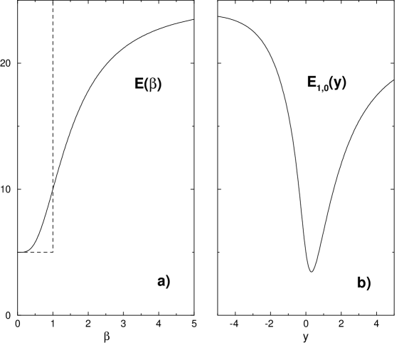
Figure 2: Energy surfaces of the critical IBM Hamiltonian $H_{cri}$ (19) with $N=5$ and $A=1$. (a) Intrinsic energy surface $E(\beta)$, Eq. (20) [solid line], and its approximation by a square-well potential [dashed line]. (b) $O(5)$ projected energy surface $E_{\xi=1,\tau=0}(y)$, Eq. (9). The global minimum is at $y=0.314$. Taken from ref.[13].

6 Comparison with E(5) and Experiment

To test the suggested procedure we compare in Table 2 the $U(5)$ decomposition of exact eigenstates obtained from numerical diagonalization of $H_{cri}$ for $N=5$ with that calculated from the $\tau$-projected states with $y=0.314$ [the global minimum of $E_{1,0}(y)$]. As can be seen, the latter provide a good approximation to the exact eigenstates (the corresponding band-mixing is $\eta_{\tau}=0.12,\,3.53,\,4.14,\,3.05\%$ for $\tau=0,1,2,3$). This agreement in the structure of wave functions is translated also into an agreement in energies and B(E2) values as shown in Table 1. The results of Table 1 and 2 clearly demonstrate the ability of the suggested procedure to provide analytic and accurate estimates to the exact finite-N calculations of the critical IBM Hamiltonian, which in-turn agree with the experimental data in ¹³⁴Ba and captures the essential features of the E(5) critical point.

Table 2: $U(5)$ decomposition (in %) of the $L^{+}_{\xi,\tau}$ states for $N=5$. The calculated values are obtained from the $\tau$-projected states, Eqs. (5), (8) with $y=0.314$. The exact values are obtained from numerical diagonalization of the critical IBM Hamiltonian $H_{cri}$, Eq. (19).

	$0^{+}_{1,0}$		$2^{+}_{1,1}$		$L^{+}_{1,2}$		$L^{+}_{1,3}$		$0^{+}_{2,0}$
$n_{d}$	calc	exact	calc	exact	calc	exact	calc	exact	calc	exact
0	83.2	83.4							15.8	16.4
1			92.2	90.2
2	16.4	16.2			96.8	95.2			70.9	76.2
3			7.8	9.7			99.1	98.4
4	0.4	0.4			3.2	4.8			13.3	7.4
5			0.0	0.1			0.9	1.6

7 Large $N$ Limit

In the large $N$ limit, using Stirling’s Formula in Eq. (6), we obtain

$$G^{(n)}_{\alpha}(y)\rightarrow 2x\,\left({x\over N}\right)^{2n}\,\sum_{p}\ \,{x^{2p}\over(2p)!!(2p+2n+1)!!}~{},$$ (21)

where $x=Ny$. Therefore,

$$S^{(N)}_{k,\tau}(y)\rightarrow{\cal S}_{k,\tau}(x)~{},$$ (22)

that is, $S^{(N)}_{k,\tau}(y)$ becomes a function of $x$ only. This suggests that the energy spectrum depends only on $x$ and not $N$ and $y$ separately as $N$ goes to infinity, except for possibly an overall scale. To test this in Fig. 3 we plot the energy ratio at the critical point

$$R={E_{\xi=1,\tau=2}-E_{\xi=1,\tau=0}\over E_{\xi=1,\tau=1}-E_{\xi=1,\tau=0}}$$ (23)

for several values of $N$ as a function of $x$. Indeed as $N$ increases, the curves asymptote to one universal curve. This means that the quadrupole beta deformation of the geometrical model is proportional to $\sqrt{N}\beta$. This observation may be useful in relating the predictions of E(5) CP to the IBM.

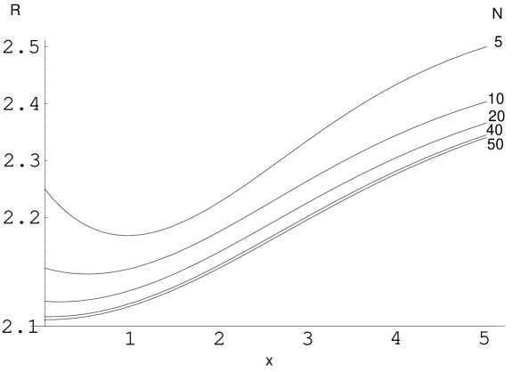
Figure 3: The energy ratio $R$ at the critical point defined in Eq. (23) as a function of $x=Ny$, for different values of N. Note that the vertical axis is displaced from zero.

8 Summary and Future Outlook

In this contribution we have examined properties of a critical point in a finite system[13]. We have focused on the E(5) critical point relevant to a second-order shape phase transition between spherical and deformed $\gamma$-unstable nuclei. At the critical point of such a phase transition the intrinsic energy surface is flat and there is no stable minimum value of the deformation. However, for a finite system, we have shown that there is an effective deformation which can describe the dynamics at the critical point. The effective deformation is determined by minimizing the energy surface after projection onto the appropriate symmetries. States of finite $N$ and good $O(5)$ symmetry, projected from intrinsic states with this effective deformation simulate accurately the exact eigenstates, and can be used to derive analytic estimates for energies and quadrupole transition rates at the critical point.

In the future we shall explore in depth the $N$-dependence as well as the large-$N$ limit and its relationship to the geometric E(5) critical point. We shall also explore the first-order critical point in the phase transition from a spherical vibrator and an axially symmetric deformed nucleus within the IBM.

References

- [1] F. Iachello, Phys. Rev. Lett. 85, 3580 (2000).
- [2] F. Iachello, Phys. Rev. Lett. 87, 052502 (2001).
- [3] R.F. Casten and N.V. Zamfir, Phys. Rev. Lett. 85, 3584 (2000).
- [4] J.M. Arias, Phys. Rev. C 63, 034308 (2001).
- [5] A. Frank, C.E. Alonso and J.M. Arias, Phys. Rev. C 65, 014301 (2002).
- [6] N.V. Zamfir, et al., Phys. Rev. C 65, 044325 (2002).
- [7] Da-li Zhang and Yu-xin Liu, Phys. Rev. C 65, 057301 (2002).
- [8] A. Arima and F. Iachello, Ann. Phys. (N.Y.) 123, 468 (1979).
- [9] M.A. Caprio, Phys. Rev. C 65, 031304 (2002).
- [10] F. Iachello and A. Arima, The Interacting Boson Model (Cambridge University Press, Cambridge, 1987).
- [11] A.E.L. Dieperink, O. Scholten and F. Iachello, Phys. Rev. Lett. 44, 1747 (1980).
-
[12]
J.N. Ginocchio and M.W. Kirson,
Phys. Rev.
Lett. 44, 1744 (1980);
J.N. Ginocchio and M.W. Kirson, Nucl. Phys. A 350, 31 (1980). - [13] A. Leviatan and J.N. Ginocchio, submitted to Phys. Rev. Lett. (2003).
- [14] T. Otsuka and M. Sugita, Phys. Rev. Lett. 59, 1541 (1987).
- [15] Yu. V. Sergeenkov, Nucl. Data Sheets 71, 557 (1994).