Intermediate energy Coulomb excitation as a probe of nuclear structure at radioactive beam facilities

Abstract

The effects of retardation in the Coulomb excitation of radioactive nuclei in intermediate energy collisions ($E_{lab}\sim 100$ MeV/nucleon) are investigated. We show that the excitation cross sections of low-lying states in ¹¹Be,^38,40,42S and ^44,46Ar projectiles incident on gold and lead targets are modified by as much as 20% due to these effects. The angular distributions of decaying gamma-rays are also appreciably modified.

I Introduction

The excitation of a nucleus by means of the electromagnetic interaction with another nucleus is known as Coulomb excitation. Since the interaction is proportional to the charge $Z$ of the nucleus, Coulomb excitation is especially useful in the collision of heavy ions, with cross sections proportional to $Z^{2}$. Pure Coulomb excitation is assured if the bombarding energy is sufficiently below the Coulomb barrier. In this case the ions follow a Rutherford trajectory and never come so close so that their nuclear matter overlaps. This mechanism has been used for many years to study the electromagnetic properties of low-lying nuclear states AW75 .

The probability for Coulomb excitation of a nuclear state $\mid f\rangle$ from an initial state $\mid i\rangle$ is large if the transition time $t_{fi}=\hbar/(E_{f}-E_{i})=1/\omega_{fi}$ is greater than the interaction time $t_{coll}=a_{0}/v$, in a heavy ion collision with closest approach distance $a_{0}$ and projectile velocity $v$. That is, the cross section for Coulomb excitation is large if the adiabacity parameter satisfies the condition

$$\xi=\frac{t_{coll}}{t_{fi}}=\omega_{fi}\dfrac{a_{0}}{v}<1\ .$$ (1)

This adiabatic cut-off limits the possible excitation energies below 1-2 MeV in sub-barrier collisions.

A possible way to overcome this limitation, and to excite high-lying states, would be the use of higher projectile energies. In this case, the closest approach distance, at which the nuclei still interact only electromagnetically, is of order of the sum of the nuclear radii, $R=R_{P}+R_{T}$, where $P$ refers to the projectile and $T$ to the target. For very high energies one has also to take into account the Lorentz contraction of the interaction time by means of the Lorentz factor $\gamma=(1-v^{2}/c^{2})^{-1/2}$, with $c$ being the speed of light. For such collisions the adiabacity condition, Eq. (1), becomes

$$\xi(R)=\frac{\omega_{fi}R}{\gamma v}<1\ .$$ (2)

¿From this relation one obtains that for bombarding energies around and above 100 MeV/nucleon, states with energy up to 10-20 MeV can be readily excited. The experimental problem is to ensure that the collision impact parameter is such that the nuclei do not overlap their matter distributions so that the process consists of Coulomb excitation only. This has been achieved by a careful filtering of the experimental events in terms of scattering angles, multiplicity of particles, angular distributions, using light and heavy targets, etc HP76 ; Mot93 ; Iek93 ; Sch93 ; Rit93 ; Gl98 ; Dav98 .

The theory of Coulomb excitation in low-energy collisions is very well understood AW75 . It has been used and improved for over thirty years to infer electromagnetic properties of nuclei and has also been tested in the experiments to a high level of precision. A large number of small corrections are now well known in the theory and are necessary in order to analyze experiments on multiple excitation and reorientation effects.

The standard semiclassical theory of Coulomb excitation at low energies assumes that the relative motion takes place on a classical Rutherford trajectory, as long as the transition energy $E_{fi}=E_{f}-E_{i}$ is small compared to the kinetic energy of the system. The cross section for exciting a definite final state $\mid f\rangle$ from the initial state $\mid i\rangle$ is then given by

$$\left(\dfrac{d\sigma}{d\Omega}\right)_{i\rightarrow f}=\left(\dfrac{d\sigma}{d\Omega}\right)_{Ruth}\cdot\;P_{i\rightarrow f}\ ,$$ (3)

where $P_{i\rightarrow f}$ is the probability, evaluated in perturbation theory, of the excitation of the target by the time-dependent electromagnetic field of the projectile AW75 .

In the case of relativistic heavy ion collisions pure Coulomb excitation may be distinguished from the nuclear reactions by demanding extreme forward scattering or avoiding the collisions in which violent reactions take place HP76 . The Coulomb excitation of relativistic heavy ions is thus characterized by straight-line trajectories with impact parameter $b$ larger than the sum of the radii of the two colliding nuclei. A detailed calculation of relativistic electromagnetic excitation on this basis was performed by Winther and Alder WA79 . As in the non-relativistic case, they showed how one can separate the contributions of the several electric ($E\lambda$) and magnetic ($M\lambda$) multipolarities to the excitation. Later, it was shown that a quantum theory for relativistic Coulomb excitation leads to minor modifications of the semiclassical results BB88 . In Ref. BN93 the connection between the semiclassical and quantum results was fully clarified. More recently, a coupled-channels description of relativistic Coulomb excitation was developed BCG02 .

The semiclassical theory of Coulomb excitation for low energy collisions accounts for the Rutherford bending of the trajectory, but relativistic retardation effects are neglected, while in the theory of relativistic Coulomb excitation recoil effects on the trajectory are neglected (one assumes straight-line motion), but retardation is handled correctly. In fact, the onset of retardation brings new important effects like the steady increase of the excitation cross sections with increasing bombarding energy. In a heavy ion collision around 100 MeV/nucleon the Lorentz factor $\gamma$ is about 1.1. Since this factor enters in the excitation cross sections in many ways, as in the adiabacity parameter, Eq. (2), one expects that some sizeable ($10-20\,\%$) modification of the theory of nonrelativistic Coulomb excitation would occur. Also, recoil corrections are not negligible, and the relativistic calculations based on a straight-line parameterization of the trajectory are not completely appropriate to describe the excitation probabilities and cross sections.

These questions are very relevant, as Coulomb excitation has proven to be a very useful tool in the investigation of rare isotopes in radioactive beam facilities Gl98 . Thus, it is appropriate to investigate the effects of retardation and recoil corrections in Coulomb excitation at intermediate and high energies. In this article we will assess these problems by using the semiclassical approach of Ref. AB89 . As we shall show in the next sections, both retardation and recoil effects must be included for bombarding energies in the range 30-200 MeV per nucleon.

This can be accomplished in a straight-forward way in the semiclassical approach with a relativistic trajectory, appropriate for heavy ion collisions, and the full expansion of the electromagnetic propagator AB89 . In most situations, the Coulomb excitation is a one-step process, which can be well described in first-order perturbation theory. Exceptions occur for very loosely bound nuclei, as for example the excitation of ¹¹Li Iek93 , or ⁸B Mot93 ; Dav98 , in which case the electromagnetic transition matrix elements are very large due to the small binding and consequent large overlap with the continuum wavefunctions. Another exception is the excitation of multiple giant resonances, due to the strong collective response of heavy nuclei to the short electromagnetic pulse delivered in heavy ion collisions at relativistic energies Sch93 ; Rit93 .

II Coulomb excitation from low to high energies

In the semiclassical theory of Coulomb excitation the nuclei are assumed to follow classical trajectories and the excitation probabilities are calculated in time-dependent perturbation theory. At low energies one uses Rutherford trajectories AW75 while at relativistic energies one uses straight-lines for the relative motion WA79 ; BB88 . In intermediate energy collisions, where one wants to account for recoil and retardation simultaneously, one should solve the general classical problem of the motion of two relativistic charged particles. A detailed study of these effects has been done in Refs. AB89 ; AAB90 . In Ref. AAB90 it was shown that the Rutherford trajectory is modified as the retardation due to the relativistic effects starts to set in. This already occurs for energies as low as 10 MeV/nucleon. It was also shown that if we use the scattering plane perpendicular to the $z$-axis, we may write the new Coulomb trajectory parameterized by

$$x=a\,\left[\cosh w+\epsilon\right];\ \ \ \ \ \ \ \ \ y=a\,\sqrt{\epsilon^{2}-1}\,\sinh w;\ \ \ \ \ \ \ \ \ \ \ z=0;\ \ \ \ \ \ \ t=\dfrac{a}{v}\,\left[w+\epsilon\,\sinh w\right]\ ,$$ (4)

where $\epsilon=1/\sin(\Theta/2)$, with $\Theta$ being the deflection angle. The impact parameter is related to the deflection angle by $b=a\cot\left(\Theta/2\right)$. The only difference from Eq. (4) and the usual parameterization of the Rutherford trajectory at non-relativistic energies is the replacement of the half-distance of closest approach in a head-on collision $a_{0}={Z_{P}Z_{T}e^{2}/}m_{0}v^{2}$ by $a=a_{0}/\gamma$. This simple modification agrees very well with numerical calculations based on the Darwin Lagrangian and the next order correction to the relativistic interaction of two charges AAB90 .

Retardation also affects the dynamics of the Coulomb excitation mechanism and needs to be included in collisions with energies around 100 MeV/nucleon and higher. A detailed account of this has been given in Ref. AB89 . The end result is that the amplitude for Coulomb excitation of a target from the initial state $\mid i\rangle$ to the final state $\mid f\rangle$ by a projectile with charge $Z_{P}$ moving along a modified Rutherford trajectory is given by

$$a_{fi}=\dfrac{Z_{P}e}{i\hbar}\sum_{\lambda\mu}\,\dfrac{4\pi}{2\lambda+1}\,(-1)^{\mu}\,\left\{S(E\lambda,\mu)\mathbf{\mathcal{M}}_{fi}(E\lambda,\,-\mu)+S(M\lambda,\mu)\mathbf{\mathcal{M}}_{fi}(M\lambda,\,-\mu)\right\}\ ,$$ (5)

where $\mathbf{\mathcal{M}}_{fi}(\pi\lambda,\mu)$ are the matrix elements for electromagnetic transitions, defined as

$$\mathbf{\mathcal{M}}_{fi}(E\lambda,\mu)={\frac{(2\lambda+1)!!}{\kappa^{\lambda+1}c(\lambda+1)}}\,\int\mathbf{j}_{fi}(\mathbf{r})\cdot\mathbf{\nabla}\times\mathbf{L}\left\{j_{\lambda}(\kappa r)\;Y_{\lambda\mu}(\vartheta,\phi)\right\}\,d^{3}r\$$ (6)

where $L=-i\mathbf{r}\times\mathbf{\nabla}$ and

$$\mathbf{\mathcal{M}}_{fi}(M\lambda,\mu)=-{\frac{i(2\lambda+1)!!}{\kappa^{\lambda}c(\lambda+1)}\ }\int\mathbf{j}_{fi}(\mathbf{r})\cdot\mathbf{L}\left\{j_{\lambda}(\kappa r)\;Y_{\lambda\mu}(\vartheta,\phi)\right\}\,d^{3}r\ ,$$ (7)

with $\omega$ defined as the excitation frequency $\hbar\omega=E_{f}-E_{i}$ and $\kappa=\omega/c$. Using the Wigner-Eckart theorem

$$\mathbf{\mathcal{M}}_{fi}(\pi\lambda,-\mu)=\left(-1\right)^{I_{f}-M_{f}}\ \left(\begin{array}[c]{ccc}I_{f}&\lambda&I_{i}\\ -M_{f}&\mu&M_{i}\end{array}\right)\ \left\langle I_{f}\left\|\mathbf{\mathcal{M}}(\pi\lambda)\right\|I_{i}\right\rangle\ ,$$ (8)

the geometric coefficients can be factorized in Eq. (5).

The orbital integrals $S(\pi\lambda,\mu$) are given by (after performing a translation of the integrand by $w\rightarrow w+i\left(\pi/2\right)$)

$$S(E\lambda,\mu) =\dfrac{\mathcal{C}_{\lambda\mu}}{va^{\lambda}}\;I(E\lambda,\mu),$$ (9)

$$S(M\lambda,\mu) =-\dfrac{{\mathcal{C}_{\lambda+1,\mu}\,}}{\lambda ca^{\lambda}}{\ [(2\lambda+1)/(2\lambda+3)]^{1/2}\,[(\lambda+1)^{2}-\mu^{2}]^{1/2}\,\cot}\left({\vartheta/2}\right){\ \ }I(M\lambda,\mu)\ ,$$

with

$$\mathcal{C}_{\lambda\mu}=\left\{\begin{array}[c]{ccl}\sqrt{\dfrac{2\lambda+1}{4\pi}}\,\dfrac{\sqrt{(\lambda-\mu)!(\lambda+\mu)!}}{(\lambda-\mu)!!(\lambda+\mu)!!}\;(-1)^{(\lambda+\mu)/2}&,&\ \ \ \ \mathrm{for}\quad\lambda+\mu=\mathrm{even}\\ 0&,&\ \ \ \ \mathrm{for}\quad\lambda+\mu=\mathrm{odd}\,\ ,\end{array}\right.$$ (10)

and

$$I(E\lambda,\mu) =-i({\frac{v\zeta}{c}})^{\lambda+1}\,{\frac{1}{\lambda(2\lambda-1)!!}}\,e^{-\pi\zeta/2}\,\int_{-\infty}^{\infty}dw\;e^{-\zeta\epsilon\cosh w}\,e^{i\zeta w}$$

$$\times\dfrac{(\epsilon+i\sinh w-\sqrt{\epsilon^{2}-1}\cosh w)^{\mu}}{(i\epsilon\sinh w+1)^{\mu-1}}$$

$$\times\left[(\lambda+1)\,h_{\lambda}-zh_{\lambda+1}-\dfrac{v}{c}\epsilon\,\zeta\,\cosh w\cdot h_{\lambda}\right]\ ,$$ (11)

and

$$I(M\lambda,\mu) =\frac{i(v\zeta/c)^{\lambda+1}}{(2\lambda-1)!!}\ e^{-\pi\zeta/2}\,\int_{-\infty}^{\infty}dw\;e^{-\zeta\epsilon\,\cosh w}e^{i\zeta w}$$

$$\times\,\dfrac{(\epsilon+i\sinh w-\sqrt{\epsilon^{2}-1}\,\cosh w)^{\mu}}{(i\epsilon\sinh w+1)^{\mu}}\ h_{\lambda}(z)\ .$$ (12)

In the above equations, all the first-order Hankel functions $h_{\lambda}$ are functions of

$$z={\frac{v}{c}}\zeta\,(i\epsilon\sinh w+1)\,,$$ (13)

with

$$\zeta=\dfrac{\omega a}{v}=\dfrac{\omega a_{o}}{\gamma v}{\ .}$$ (14)

The square modulus of Eq. (5) gives the probability of exciting the target from the initial state $\mid I_{i}M_{i}\rangle$ to the final state $\mid I_{f}M_{f}\rangle$ in a collision with the center of mass scattering angle $\vartheta$. If the orientation of the initial state is not specified, the cross section for exciting the nuclear state of spin $I_{f}$ is

$$d\sigma_{i\rightarrow f}=\frac{a^{2}\epsilon^{4}}{4}\;\frac{1}{2I_{i}+1}\;\sum_{M_{i},M_{f}}\mid a_{fi}\mid^{2}\,d\Omega\,,$$ (15)

where $a^{2}\epsilon^{4}d\Omega/4$ is the elastic (Rutherford) cross section. Using the Wigner-Eckart theorem, Eq. (8), and the orthogonality properties of the Clebsch-Gordan coefficients, gives

$${\frac{d\sigma_{i\rightarrow f}}{d\Omega}}=\frac{4\pi^{2}Z_{P}^{2}e^{2}}{\hbar^{2}}\;a^{2}\epsilon^{4}\;\sum_{\pi\lambda\mu}{\dfrac{B(\pi\lambda,I_{i}\rightarrow I_{f})}{(2\lambda+1)^{3}}}\;\mid S(\pi\lambda,\mu)\mid^{2}\ ,$$ (16)

where $\pi=E$ or $M$ stands for the electric or magnetic multipolarity, and

$$B(\pi\lambda,I_{i} \longrightarrow I_{f})=\dfrac{1}{2I_{i}+1}\;\sum_{M_{i},M_{f}}\mid\mathcal{M}(\pi\lambda,\mu)\mid^{2}\$$

$$=\frac{1}{2I_{i}+1}\ \left|\left\langle I_{f}\left\|\mathbf{\mathcal{M}}(\pi\lambda)\right\|I_{i}\right\rangle\right|^{2}\$$ (17)

is the reduced transition probability.

III Relativistic and non-relativistic limits

The non-relativistic limit is readily obtained by using $v/c\rightarrow 0$ in the expressions in section II. In this case, $z\rightarrow 0$ in Eq. (13), and

$$h_{\lambda} \rightarrow-i\left(2\lambda-1\right)!!\frac{1}{z^{\lambda+1}}$$

$$(\lambda+1)\,h_{\lambda}-zh_{\lambda+1}-\dfrac{v}{c}\epsilon\,\zeta\,\cosh w\cdot h_{\lambda} \rightarrow i\lambda\left(2\lambda-1\right)!!\frac{1}{z^{\lambda+1}}\ ,$$ (18)

which yields

$$I(E\lambda,\mu) =\,e^{-\pi\zeta/2}\,\int_{-\infty}^{\infty}dw\;e^{-\zeta\epsilon\cosh w+i\zeta w}\dfrac{(\epsilon+i\sinh w-\sqrt{\epsilon^{2}-1}\cosh w)^{\mu}}{(i\epsilon\sinh w+1)^{\lambda+\mu}},$$ (19)

$$I(M\lambda,\mu) =I(E\lambda+1,\mu)\ .$$ (20)

These are indeed the orbital integrals for non-relativistic Coulomb excitation, as defined in Eq. (II-E.49) of Ref. AW65 .

In the relativistic limit, $v/c\rightarrow 1,$ $\zeta\rightarrow 0$ in Eq. (14) and $\epsilon\simeq b/a\rightarrow\infty$. However, the combination

$$\xi(b)=\zeta\epsilon=\frac{\omega_{fi}b}{\gamma v}$$ (21)

can remain finite.

The results for the orbital integrals can be expressed in closed analytical forms. First we translate back the integrands in Eqs. (11) and (12) by $-i\left(\pi/2\right)$ to get

$$I(E\lambda,\mu) =-i({\frac{v\zeta}{c}})^{\lambda+1}\epsilon{\frac{1}{\lambda(2\lambda-1)!!}}\,\int_{-\infty}^{\infty}dw\;e^{i\xi\sinh w}\,\dfrac{(1+i\sinh w)^{\mu}}{(\cosh w)^{\mu-1}}$$

$$\times\left[(\lambda+1)\,h_{\lambda}-zh_{\lambda+1}+i\dfrac{v}{c}\xi\sinh w\cdot h_{\lambda}\right]\ ,$$ (22)

and

$$I(M\lambda,\mu)=\frac{i(v\zeta/c)^{\lambda+1}}{(2\lambda-1)!!}\ \,\int_{-\infty}^{\infty}dw\;h_{\lambda}(z)\;e^{i\xi\,\sinh w}\dfrac{(1+i\sinh w)^{\mu}}{(\cosh w)^{\mu}}\ ,$$ (23)

where now $z={\dfrac{v}{c}}\xi\cosh w$, and we took the limit $\zeta\rightarrow 0$ and $\epsilon\rightarrow\infty.$ For the lowest multipolarities these integrals can be obtained in terms of modified Bessel functions by assuming the long-wavelength approximation, $\xi\left(R\right)\ll 1$, valid for almost all cases of practical interest. In this case, we can also use the approximation of Eqs. (18). From Eq. (4), in the relativistic limit, $\sinh w=vt/b$ and $r=b\cosh w$. Thus, the integrals can be rewritten as

$$I(E\lambda,\mu) =va^{\lambda}\,e^{-\pi\zeta/2}\int_{-\infty}^{\infty}dt\;e^{i\xi vt/b}\,\dfrac{(b+ivt)^{\mu}}{(b^{2}+v^{2}t^{2})^{\left(\lambda+\mu+1\right)/2}}\left[1-i\frac{vt}{\lambda b}\dfrac{v}{c}\xi\right]\ ,$$ (24)

$$I(M\lambda,\mu) =va^{\lambda+1}\ e^{-\pi\zeta/2}\,\int_{-\infty}^{\infty}dt\;e^{i\xi vt/b}\,\dfrac{(b+ivt)^{\mu}}{(b^{2}+v^{2}t^{2})^{\left(\lambda+\mu+2\right)/2}}\ .$$ (25)

These integrals can be calculated analytically GR65 to give

$$I(E\lambda,\mu)=F(\lambda,\mu,\xi)-\dfrac{v}{\lambda c}\xi\frac{dF(\lambda,\mu,\xi)}{d\xi},\ \ \ \ \ \ \ \ \ \ \ I(M\lambda,\mu)=F(\lambda+1,\mu,\xi)$$ (26)

where

$$F(\lambda,\mu,\xi)=2\left(-1\right)^{\frac{\lambda+\mu}{2}}\left(\frac{a}{b}\xi\right)^{\lambda}\sum_{n=-\lambda}^{\lambda}\frac{1}{2^{n}}\left(-1\right)^{n-\mu}\frac{P_{\lambda-n}^{\left(n-\mu,\ n+\mu\right)}\left(0\right)}{P_{\lambda}^{\left(-\mu,\ \mu\right)}\left(0\right)}K_{n}\left(\xi\right)\ .$$ (27)

In this equation $P_{n}^{\left(\alpha,\beta\right)}$ are the Jacobi polynomials, and $K_{n}\left(x\right)$ are modified Bessel functions. Since $\lambda+\mu=$even (odd) for electric (magnetic) excitations, we only need to calculate the integrals for $\mu=\pm 1$ for the E1 multipolarity, $\mu=0,\pm 2$ for the E2 multipolarity, and $\mu=0$ for the M1 multipolarity, respectively.

To leading order in $\xi$,

$$I(E1,\pm 1) =\frac{2a}{b}\mathcal{I}\left(\xi\right),\ \ \ \ \ I(M1,0)=I(E2,0)=\frac{2a^{2}}{b^{2}}\mathcal{I}\left(\xi\right),\ \ \ \ \ \ \ I(E2,\pm 2)=\frac{2a^{2}}{3b^{2}}\mathcal{I}\left(\xi\right).$$

$$\mathcal{I}\left(\xi\right) =\xi K_{1}\left(\xi\right)=\left\{\begin{array}[c]{lll}1,&\mathrm{for}&\ \ \ \ \ \xi\lesssim 1\\ 0,&\mathrm{for}&\ \ \ \ \ \xi\gtrsim 1\ .\end{array}\right.$$ (30)

When inserted in Eqs. (9) and (16) the above results yield the correct relativistic Coulomb excitation cross sections WA79 in the long wavelength approximation. Thus, we have shown explicitly that the Equations (4)-(16) reproduce the non-relativistic and relativistic Coulomb excitation expressions, as proved numerically in Ref. AB89 . We can now analyze the intermediate energy region ($E_{Lab}\sim 100$ MeV/nucleon), where most experiments with radioactive beams are being performed.

IV Gamma-ray angular distributions

As for the non-relativistic case WB65 ; AW65 , the angular distributions of gamma rays following the excitation depend on the frame of reference considered. It is often more convenient to express the angular distribution of the gamma rays in a coordinate system with the $z$-axis in the direction of the incident beam. This amounts in doing a transformation of the excitation amplitudes by means of the rotation functions $D_{m^{\prime}m}^{j}$. The final result is identical to the Eqs. (II.A.66-77) of Ref. AW65 , with the non-relativistic orbital integrals replaced by Eqs. (11) and (12), respectively. The angular distribution of the gamma rays emitted into solid angle $\Omega_{\gamma}$, as a function of the scattering angle of the projectile ($\Theta,\Phi$), is given by

$$W\left(\Omega_{\gamma}\right)=\sum_{k\kappa}a_{k\kappa}^{\lambda}\left(\Theta,\Phi,\zeta\right)A_{k}^{(\lambda)}Y_{k\kappa}\left(\Omega_{\gamma}\right)\ .$$ (31)

In our notation, the $z$-axis corresponds to the beam axis, and the $a_{k\kappa}^{\lambda}\left(\Theta,\Phi,\zeta\right)$ are given by

$$a_{k\kappa}^{\lambda}\left(\Theta,\Phi,\zeta\right)=b_{k\kappa}^{\lambda}/b_{00}^{\lambda}\ ,$$ (32)

where, for electric excitations AW65 ,

$$b_{k\kappa}^{E\lambda}\left(\Theta,\Phi,\zeta\right) =-\frac{2}{\sqrt{2k+1}}\left(\begin{array}[c]{ccc}\lambda&\lambda&k\\ 1&-1&0\end{array}\right)^{-1}\sum_{\mu\mu^{\prime}\kappa^{\prime}}\left(-1\right)^{\mu}\left(\begin{array}[c]{ccc}\lambda&\lambda&k\\ \mu&-\mu^{\prime}&\kappa^{\prime}\end{array}\right)$$ (37)

$$\times Y_{\lambda\mu}\left(\frac{\pi}{2},0\right)Y_{\lambda\mu^{\prime}}\left(\frac{\pi}{2},0\right)\ I(E\lambda,\mu)I(E\lambda,\mu^{\prime})D_{\kappa^{\prime}\kappa}^{k}\left(\frac{\pi}{2}+\frac{\Theta}{2},\frac{\pi}{2},\Phi\right)\ .$$ (38)

In Eq. (31) the coefficients $A_{k}^{(\lambda)}$ are given by

$$A_{k}^{(\lambda)}=F_{k}\left(\lambda,I_{i},I_{f}\right)\sum_{ll^{\prime}}F_{k}\left(l,l^{\prime},I_{g},I_{f}\right)\Delta_{l}\Delta_{l^{\prime}}\ ,$$ (39)

where $\left|\Delta_{l}\right|^{2}$ is the intensity (in sec^-1) of the 2^l-pole radiation in the $\gamma$-transition from the excited state $g$ to the state $f$. Explicitly, the $l$-pole conversion coefficient $\Delta_{l}$ is given by

$$\Delta_{\pi l}=\left[\frac{8\pi\left(l+1\right)}{l\left[\left(2l+1\right)!!\right]^{2}}\frac{1}{\hbar}\left(\frac{\omega}{c}\right)^{2l+1}\right]^{1/2}\left(2I_{f}+1\right)^{-1/2}\left\langle I_{f}\left\|i^{s(l)}\mathcal{M}(\pi l)\right\|I_{g}\right\rangle\ ,$$ (40)

with $s(l)=l$ for electric $\left(\pi=E\right)$ and $s(l)=l+1$ for magnetic $\left(\pi=M\right)$ transitions. The product $\Delta_{l}\Delta_{l^{\prime}}$ is always real since $\left(-1\right)^{s(l)}=$ (the parity). The coefficients $F_{k}\left(l,l^{\prime},I_{g},I_{f}\right)$ are geometrical factors defined by

$$F_{k}\left(l,l^{\prime},I_{g},I_{f}\right) =\left(-1\right)^{I_{f}+I_{g}-1}\sqrt{\left(2l+1\right)\left(2l^{\prime}+1\right)\left(2I_{f}+1\right)\left(2k+1\right)}$$

$$\times\left(\begin{array}[c]{ccc}l&l^{\prime}&k\\ 1&-1&0\end{array}\right)\left\{\begin{array}[c]{ccc}l&l^{\prime}&k\\ I_{f}&I_{f}&I_{g}\end{array}\right\}\ ,$$ (45)

and

$$F_{k}\left(l,I_{i},I_{f}\right)=F_{k}\left(l,l,I_{i},I_{f}\right).$$ (46)

The normalization of the coefficients $a_{k\kappa}^{\lambda}\left(\Theta,\Phi,\zeta\right)$ is such that $a_{00}^{\lambda}\left(\Theta,\Phi,\zeta\right)=1.$ Only terms with even $k$ occur in Eq. (31).

The total angular distribution of the gamma rays, which integrates over all scattering angles of the projectile, is given by

$$W\left(\theta_{\gamma}\right)=\sum_{k}a_{k}^{\lambda}\left(\zeta\right)A_{k}^{(\lambda)}P_{k}\left(\cos\theta_{\gamma}\right)\ ,$$ (47)

where the $z$-axis corresponds to the beam axis and the statistical tensors are given by

$$a_{k}^{\lambda}\left(\zeta\right)=b_{k}^{\lambda}/b_{0}^{\lambda}\ ,$$ (48)

where (for electric excitations) AW65 ,

$$b_{k}^{E\lambda}\left(\zeta\right) =-\frac{2}{\sqrt{2k+1}}\left(\begin{array}[c]{ccc}\lambda&\lambda&k\\ 1&-1&0\end{array}\right)^{-1}\sum_{\mu\mu^{\prime}\kappa}\left(-1\right)^{\mu}\left(\begin{array}[c]{ccc}\lambda&\lambda&k\\ \mu&-\mu^{\prime}&\kappa\end{array}\right)$$ (53)

$$\times Y_{\lambda\mu}\left(\frac{\pi}{2},0\right)Y_{\lambda\mu^{\prime}}\left(\frac{\pi}{2},0\right)\int_{\epsilon_{0}}^{\infty}d\epsilon\ \epsilon\ I(E\lambda,\mu)I(E\lambda,\mu^{\prime})Y_{k\kappa}\left(\frac{\pi}{2},\frac{\pi}{2}+\sin^{-1}\left(1/\epsilon\right)\right)\ .$$ (54)

$\epsilon_{0}$ is the minimum value of the eccentricity, associated with the maximum scattering angle $\Theta_{0}$ by $\epsilon_{0}=1/\sin\left(\Theta_{0}/2\right)$. One can show that the coefficients $b_{k}^{E\lambda}$ are real, even if the orbital integrals are not. Their imaginary parts cancel out in the sum over $\mu\mu^{\prime}$.

For $M1$ excitations

$$b_{k}^{M1} =-\frac{8}{\sqrt{2k+1}}\left(\begin{array}[c]{ccc}1&1&k\\ 1&-1&0\end{array}\right)^{-1}\left(\begin{array}[c]{ccc}1&1&k\\ 0&0&0\end{array}\right)\left[Y_{20}\left(\frac{\pi}{2},0\right)\right]^{2}$$ (59)

$$\int_{\epsilon_{0}}^{\infty}d\epsilon\ \epsilon\ \left(\epsilon^{2}-1\right)\ I(M1,0)I(M1,0)Y_{k0}\left(\frac{\pi}{2},\frac{\pi}{2}+\sin^{-1}\left(1/\epsilon\right)\right).$$ (60)

The normalization of the coefficients $a_{k}^{\lambda}\left(\zeta\right)$ is such that $a_{0}^{\lambda}\left(\zeta\right)=1.$ Again, only terms with even $a_{k}^{\lambda}\left(\zeta\right)$ occur in Eq. (47).

In the case of $M1$ excitations Eq. (60) contains only $\kappa=\mu=\mu^{\prime}=0$ and one gets $a_{2}^{M1}\left(\zeta\right)=1,$ independent of $\zeta$. Since for small $\zeta$ the magnitude of $a_{k}^{\lambda}\left(\zeta\right)$ decreases appreciably with $k$ we will only consider gamma ray emission after excitation through electric multipoles, in particular, the dependence of $a_{2}^{E1}$ and $a_{2}^{E2}$ on $\zeta$. This dependence is very weak at energies $E_{lab}\gtrsim 100$ MeV/nucleon. In that case, one can use the approximate relations, Eq. (30), for excitation energies such that $\xi\ll 1$. This condition is met for reactions with neutron-rich or proton-rich nuclei where the excitation energies involved are of the order of $E_{x}\sim 1$ MeV. It is then straightforward to show that

$$a_{2}^{E1}=1,\ \ \ \ \ a_{2}^{E2}=-2,\ \ \ \ \ \ \ \text{\ and}\ \ \ \ a_{4}^{E2}=-0.25.$$ (61)

We thus come to the important conclusion that in high energy collisions and low excitation energies, $E_{x}\sim 1$ MeV, the angular distribution of gamma-rays from decays after Coulomb excitation does not depend on the parameters $\zeta$ or $\xi$.

Although the cross sections for $M1$ and $E2$ excitations do not contain interference terms, the $\gamma$-decay of the excited state can contain an interference term with mixed $E2+M1$ multipolaritites. The angular distribution of the gamma rays from the deexcitation of these states is given by AW65

$$W^{E2,M1}\left(\theta_{\gamma}\right)=2\sqrt{\sigma_{M1}}\sqrt{\sigma_{E2}}\sum_{k}a_{k}^{E2,M1}\left(\zeta\right)F_{k}\left(1,2,I_{i},I_{f}\right)\sum_{ll^{\prime}}\Delta_{l}\Delta_{l^{\prime}}F_{k}\left(l,l^{\prime},I_{g},I_{f}\right)P_{k}\left(\cos\theta_{\gamma}\right)\ ,$$ (62)

where $\sigma_{M1}$ ($\sigma_{E2}$) is the total magnetic dipole (electric quadrupole) excitation cross section and where the sign of the square root is the same as the sign of the reduced matrix element $\left\langle i\left\|\mathcal{M}\left(M1\right)\right\|f\right\rangle$ ($\left\langle i\left\|\mathcal{M}\left(E2\right)\right\|f\right\rangle$). These latter are the same as those occurring in the radiative decay $f\longrightarrow i$. The $a_{k}^{E2,M1}$ coefficients in Eq. (62) are given by

$$a_{k}^{E2,M1}=b_{k}^{E2,M1}/\sqrt{b_{0}^{E2}}\sqrt{b_{0}^{M1}}\ ,$$ (63)

where $b_{k}^{\lambda}$ is given by Eq. (54) and

$$b_{k}^{E2,M1} =-\frac{4}{\sqrt{2k+1}}\left(\begin{array}[c]{ccc}2&1&k\\ 1&-1&0\end{array}\right)^{-1}\sum_{\mu}\left(-1\right)^{\mu}\left(\begin{array}[c]{ccc}2&1&k\\ \mu&0&\mu\end{array}\right)$$ (68)

$$\times Y_{2\mu}\left(\frac{\pi}{2},0\right)Y_{20}\left(\frac{\pi}{2},0\right)\int_{\epsilon_{0}}^{\infty}d\epsilon\ \epsilon\ \sqrt{\epsilon^{2}-1}\ I(E2,\mu)I(M1,0)Y_{k\mu}\left(\frac{\pi}{2},\frac{\pi}{2}+\sin^{-1}\left(1/\epsilon\right)\right)\ .$$ (69)

Using the relations in Eq. (30) and performing the summation above it is straightforward to show that for $\xi(R)\ll 1$

$$a_{k}^{E2,M1}=0,\ \ \ \ \mathrm{for\ any}\ k\ .$$

Thus, in high-energy collisions, there is no interference term from mixed E2-M1 excitations in the angular distribution of emitted gamma rays.

The form of the expressions for the angular distribution used here has followed that of Chapter 11 of Ref. AW65 . Experimenters usually find it more convenient to write the angular distribution in a slightly different form which separates the statistical tensors that describe the orientation of the state due to the excitation process from the geometrical factors associated with the $\gamma$-ray decay and gives the geometrical factors the same form as occurs in the formulation of $\gamma$-$\gamma$ correlations (cf. Ref. AW65 page 311; see also Refs. stu02 ; stu03 ). The general expression for the $\gamma$-ray decay into solid angle $\Omega_{\gamma}$ after projectile scattering to the angle $(\Theta,\Phi)$, where the transition takes place between the Coulomb-excited state $f$ and a lower state $g$ (see Eq. (31)) becomes:

$$W\left(\Omega_{\gamma}\right)=\sum_{k\kappa}\alpha_{k\kappa}^{\lambda}\left(\Theta,\Phi,\zeta\right)A_{k}(\delta_{\gamma}ll^{\prime}I_{g}I_{f})Q_{k}(E_{\gamma})Y_{k\kappa}\left(\Omega_{\gamma}\right)\ ,$$ (70)

where the $A_{k}(\delta_{\gamma}ll^{\prime}I_{g}I_{f})$ coefficients are related to the so-called $F$-coefficient (Eq. (45)) for the $\gamma$-ray transition between the states $I_{f}$ and $I_{g}$ with mixed multipolarities $l$ and $l^{\prime}$ and mixing ratio $\delta_{\gamma}$ kra73 ; AW65 by the expression

$$A_{k}(\delta_{\gamma}ll^{\prime}I_{f}I_{g})=[F_{k}(llI_{f}I_{g})+2\delta_{\gamma}F_{k}(ll^{\prime}I_{f}I_{g})+\delta_{\gamma}^{2}F_{k}(l^{\prime}l^{\prime}I_{f}I_{g})]/(1+\delta_{\gamma}^{2}).$$ (71)

Note that for $k=0$ we have $A_{0}=F_{0}=1$, and due to the normalization used, the matrix elements, Eq. (40), are not needed. In most situations one is interested in the possible mixing of $E2$ and $M1$ multipolarities in the decay of $f\longrightarrow g$. Thus, one only needs the $E2/M1$ mixing ratio. The quantity $Q_{k}(E_{\gamma})$ is the solid-angle attenuation coefficient which takes account of the finite solid-angle opening of the $\gamma$-ray detector yates . It follows that

$$\alpha_{k\kappa}^{\lambda}\left(\Theta,\Phi,\zeta\right)=a_{k\kappa}^{\lambda}\left(\Theta,\Phi,\zeta\right)F_{k}(\lambda\lambda I_{i}I_{f}).$$ (72)

In the case where the particle scatters into an annular counter about the beam direction (i.e. the $z$-axis), or for angular distributions where the scattered particle is not detected at all (Eq. (47)), only $\kappa=0$ terms survive. Usually the coefficients are normalized so that

$$W(\theta_{\gamma})=1+\sum_{k=2,4}B_{k}^{\lambda}\left(\zeta\right)A_{k}(\delta_{\gamma}ll^{\prime}I_{g}I_{f})Q_{k}(E_{\gamma})P_{k}\left(\cos\theta_{\gamma}\right).$$ (73)

The alignment of the initial state is now specified by the statistical tensor $B_{k}^{\lambda}$ which is related to the statistical tensors introduced above by

$$B_{k}^{\lambda}=\sqrt{2k+1}\;\alpha^{\lambda}_{k0}/\alpha^{\lambda}_{00},$$ (74)

when the particle is detected in an annular counter, and

$$B_{k}^{\lambda}=a_{k}^{\lambda}\left(\zeta\right)F_{k}(\lambda\lambda I_{i}I_{f}),$$ (75)

when the particle is not detected at all (or detected in such a way as to include all kinematically allowed scattering angles).

V Numerical results

In Table 1 we show the numerical results for the orbital integral $I(E2,\mu)$ for a deflection angle of 10⁰ and for $\mu=2,0,-2$. The calculations have been done using the code COULINT Ber03 . The results for $\gamma=1$ agree within 1/1000 with the numerical values obtained in Ref. AW56 , also reprinted in Table II.12 of Ref. AW65 . One observes that the results of the integrals for $\gamma=1.1,$ corresponding to a laboratory energy of about 100 MeV/nucleon, differ substantially from the results for $\gamma=1$ (non-relativistic), specially for large values of $\zeta$. For a fixed scattering angle $\zeta$ increases with the excitation energy. Thus, one expects that the relativistic corrections are greater as the excitation energy increases.

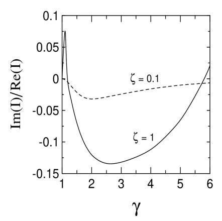
For $\gamma=1$ the imaginary part of the orbital integrals vanishes. But as $\zeta$ and $\gamma$ increase the imaginary part becomes important. This is shown in Fig. 1 where the ratio of the imaginary to real parts of the orbital integral $I(E2,2)$ is shown for $\zeta=0.1$ (dashed curve) and $\zeta=1$ (solid curve) as a function of $\gamma$.

Except for the very low energies such that $a_{0}$ attains a large value, and for the very large excitation energies $\hbar\omega$, the parameter $\zeta$ is much smaller than unity. Also, at intermediate energies the scattering angle is limited to very forward scattering. It is useful to compare the orbital integrals with their limiting expressions given by Eq. (30), i.e. the relativistic limit to leading order in $\xi$. This is shown in Fig. 3(a) where the real (solid lines) and imaginary parts (long-dashed lines) of the orbital integral $I(E1,1)$ are compared to the approximation of Eq. (30) (dashed line) for $\gamma=1.1$ ($E_{\mathrm{lab}}\simeq 100$ MeV/nucleon). Figure 3(b) shows the same results, but for the orbital integral $I(E2,2)$. The comparison is made in terms of the variable $\xi=\epsilon\zeta$  which is the appropriate variable for high energy collisions. Only for $\xi\ll 1$ do the expressions in the relativistic limit reproduce the correct behavior of the orbital integrals. Although the imaginary parts of the orbital integrals are small, the real parts show substantial deviations from the approximations of Eq. (30) at intermediate energies ($E_{\mathrm{lab}}\simeq 100$ MeV/nucleon).

$\zeta$	$\ \ \ \ \ \ \lambda,\mu=2,2$	$\ \ \ \ \ \ \ \ \lambda,\mu=2,0$	$\ \ \ \ \ \ \ \lambda,\mu=2,-2$
0.0	5.064(-3) [5.052(-3)]	1.332(-2) [1.332(-2)]	5.064(-3) [5.073(-3)]
0.1	8.675(-4) [1.105(-3)]	6.505(-3) [7.621(-3)]	1.195(-2) [1.205(-2)]
0.2	1.895(-4) [2.897(-4)]	2.280(-3) [3.276(-3)]	7.765(-3) [9.487(-3)]
0.3	4.425(-5) [7.849(-5)]	7.311(-4) [1.296(-3)]	2.245(-3) [5.470(-3)]
0.4	1.069(-5) [2.122(-5)]	2.245(-4) [4.920(-4)]	1.468(-3) [2.728(-3)]
0.5	2.637(-6) [5.599(-6)]	6.716(-5) [1.821(-4)]	5.442(-4) [1.251(-3)]
0.6	6.598(-7) [1.402(-6)]	1.975(-5) [6.627(-5)]	1.908(-4) [5.431(-4)]
0.7	1.668(-7) [3.169(-7)]	5.739(-6) [2.383(-5)]	6.438(-5) [2.268(-4)]
0.8	4.250(-8) [5.580(-8)]	1.652(-6) [8.492(-6)]	2.110(-5) [9.201(-5)]
0.9	1.090(-8) [1.906(-9)]	4.724(-7) [3.004(-6)]	6.765(-6) [3.650(-5)]
1.0	2.807(-9) [-5.003(-9)]	1.343(-7) [1.057(-6)]	2.131(-6) [1.422(-5)]
1.2	1.886(-10) [-1.845(-9)]	1.071(-8) [1.291(-7)]	2.031(-7) [2.074(-6)]
1.4	1.282(-11) [-3.551(-10)]	8.426(-10) [1.556(-8)]	1.858(-8) [2.902(-7)]
1.6	8.788(-13) [-5.699(-11)]	6.566(-11) [1.857(-9)]	1.651(-9) [3.941(-8)]
1.8	6.068(-14) [-8.381(-12)]	5.078(-12) [2.200(-10)]	1.433(-10) [5.227(-9)]
2.0	4.213(-15) [-1.170(-12)]	3.904(-13) [2.591(-11)]	1.222(-11) [6.809(-10)]
4.0	1.294(-26) [-1.211(-21)]	2.362(-24) [1.111(-20)]	1.464(-22) [5.663(-19)]

Table 1: The classical orbital integrals for E2 Coulomb excitation. The Table lists the values of the classical orbital integrals $I(E2,\mu)$ for a deflection angle of 10^∘ and for $\mu=2,0,-2$. These entries are given in the form of a number followed by the power of ten which it should be multiplied. The value outside (inside) the brackets are for $\gamma=1$ ($\gamma=1.1$).

We now apply the formalism to specific cases. We study the effects of relativistic corrections in the collision of the radioactive nuclei ^38,40,42S and ^44,46Ar on gold targets. These reactions have been studied at $E_{lab}\sim 40$ MeV/nucleon at the MSU facility Sch96 . In the following calculations the conditions may be such that there will be contributions from nuclear excitation, but these will be neglected as we only are interested in the relativistic effects in Coulomb excitation at intermediate energy collisions. In Table 2 we show the Coulomb excitation cross sections of the first excited state in each nucleus as a function of the bombarding energy per nucleon. The cross sections are given in milibarns. The numbers inside parenthesis and brackets were obtained with pure non-relativistic and relativistic calculations respectively. The minimum impact parameter is chosen so that the distance of closest approach corresponds to the sum of the nuclear radii in a collision following a Rutherford trajectory. One observes that at 10 MeV/nucleon the relativistic corrections are important only at the level of 1%. At 500 MeV/nucleon, the correct treatment of the recoil corrections (included in the equations (11) and (12)) is relevant on the level of 1%. Thus the non-relativistic treatment of Coulomb excitation WB65 can be safely used for energies below about 10 MeV/nucleon and the relativistic treatment with a straight-line trajectory WA79 is adequate above about 500 MeV/nucleon. However at energies around 50 to 100 MeV/nucleon, accelerator energies common to most radioactive beam facilities (MSU, RIKEN, GSI, GANIL), it is very important to use a correct treatment of recoil and relativistic effects, both kinematically and dynamically. At these energies, the corrections can add up to 50%. These effects were also shown in Ref. AB89 for the case of excitation of giant resonances in collisions at intermediate energies. As shown here, they are also relevant for the low-lying excited states.

Figure 1: The ratio of the imaginary to real parts of the orbital integral $I(E2,2)$ is shown for $\varsigma=0.1$ (dashed curve) and $\zeta=1$ (solid curve) as a function of $\gamma$.

As another example, we calculate the Coulomb excitation cross sections of ¹¹Be projectiles on lead targets. ¹¹Be is a one neutron halo-nucleus with one excited bound state ($\frac{1}{2}^{-}$ at 320 keV). Its $\frac{1}{2}^{+}$ ground state is strongly coupled to the excited state with the strongest E1 transition observed between bound nuclear states. The B(E1) value for this transition is 0.116 e² fm² Mil83 . The one-neutron separation energy is only 506 keV and the coupling to the continuum has to be included in an accurate calculation. However the influence of higher-order effects in the Coulomb excitation of the excited state in intermediate energy collisions was shown in Refs. BCH95 ; BT95 ; SKY96 to be less than 7%. We thus neglect these effects here.

In Ref. WA79 a recoil correction for the theory of relativistic Coulomb excitation was proposed. It was shown that one can use the equations for relativistic Coulomb excitation and obtain reasonable results for collisions at low energies if one replaces the impact parameter $b$ by

$$b^{\prime}=b+{\pi\over 2}a\ .$$ (76)

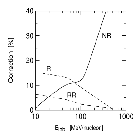
The advantage of this approximation is that one can use the analytical formulas for relativistic Coulomb excitation (e.g., Eqs. 26-27) and easily include the recoil correction Eq. (76). We define the percent deviation

$$\Delta_{i}={(\sigma_{\rm exact}-\sigma_{i})\over\sigma_{\rm exact}}$$ (77)

where $\sigma_{i}$ is the cross section obtained with the relativistic ($i=R$), non-relativistic ($i=NR$), and ($i=RR$) with the relativistic equations for Coulomb excitation Eq. (26) but with the recoil correction Eq. (76), respectively. Figure 2 is a plot of Eq. (77) for the excitation of the 0.89 MeV state in ⁴⁰S + ¹⁹⁷Au collisions as a function of the bombarding energy. One observes that the largest discrepancy is obtained by using the non-relativistic equations (NR) for the Coulomb excitation cross sections at high energies. The relativistic analytical equations (R) also do not do a good job at low energies, as expected. But the relativistic equations with the recoil correction of Eq. (76) improve considerably the agreement with the exact calculation. At 10 MeV/nucleon the deviation from the exact calculation amounts to 6% for the case shown in Fig. 2. However, the deviation of the RR treatment tends to increase for cases where higher nuclear excitation energies are involved AB89 . The cross section for the excitation of low energy states is mainly due to collisions with large impact parameters for which recoil corrections are not relevant. For high lying states, e.g. giant resonances, only the smaller impact parameters are effective in the excitation process. Therefore, in this situation, the correct treatment of recoil effects is more relevant.

Figure 2: Eq. (77) for the excitation of the 0.89 MeV state in ⁴⁰S + ¹⁹⁷Au collisions as a function of the bombarding energy. The solid line corresponds to the use of the non-relativistic integrals Eq. (19) compared to the exact calculation using Eq. (11). The same is plotted for the other two cases: (R) with the relativistic Eq. (26), and (RR) with the relativistic Eq. (26) using the recoil correction Eq. (76).

For ¹¹Be projectiles on lead targets at 50 MeV/nucleon the Coulomb excitation cross sections of the excited state in ¹¹Be are given by 311 mb, 305 mb and 398 mb for non-relativistic, exact, and relativistic calculations, respectively. At 100 MeV/nucleon the same calculations lead to 159 mb, 185 mb and 225 mb, respectively. Thus, the same trend as in the results of Table 2 is also observed for E1 excitations of low-lying states.

Experiments of Coulomb excitation of ¹¹Be projectiles have been performed at GANIL (43 MeV/nucleon) Ann95 , at RIKEN (64 MeV/nucleon) Nak97 and at MSU (57-60 MeV/nucleon) Fau97 . The extracted values of $B(E1)\sim 0.05$ e² fm² in the GANIL experiment is in disagreement with the lifetime experiment of Ref. Mil83 and could not be explained by higher-order effects in Coulomb excitation at intermediate energy collisions BCH95 ; BT95 ; SKY96 . However, the deduced values of $B(E1)\sim 0.1$ e² fm² in the RIKEN and MSU experiments are in good agreement with the lifetime measurement Mil83 and with the theoretical cross sections of Coulomb excitation.

Figure 3: Upper figure: Real (solid lines) and imaginary part (long-dashed lines) of the orbital integral $I(E1,1)$ for $\gamma=1.1$ ($E_{\mathrm{lab}}\simeq 100$ MeV/nucleon). The approximation of Eq. (30) is shown by the dashed line. Lower figure: Same plot, but for the orbital integral $I(E2,2)$.

Nucleus	Ex	B(E2)	10 MeV/A	50 MeV/A	100 MeV/A	500 MeV/A
	[MeV]	[e2fm4]	$\sigma_{C}$ [mb]	$\sigma_{C}$ [mb]	$\sigma_{C}$ [mb]	$\sigma_{C}$ [mb]
38S	1.29	235	(492) 500 [651]	(80.9) 91.7 [117]	(40.5) 50.1 [57.1]	(9.8) 16.2 [16.3]
40S	0.89	334	(877) 883 [1015]	(145.3) 162 [183]	(76.1) 85.5 [93.4]	(9.5) 20.9 [21.]
42S	0.89	397	(903) 908 [1235]	(142.7) 158 [175]	(65.1) 80.1 [89.4]	(9.9) 23.2 [23.4]
44Ar	1.14	345	(747) 752 [985]	(133) 141 [164]	(63.3) 71.7 [80.5]	(8.6) 17.5 [17.6]
46Ar	1.55	196	(404) 408 [521]	(65.8) 74.4 [88.5]	(30.2) 37.4 [41.7]	(5.72) 10.8 [11]

Table 2: Coulomb excitation cross sections of the first excited state in ^38,40,42S and ^44,46Ar projectiles at 10, 50 100 and 500 MeV/nucleon incident on gold targets. The numbers inside parenthesis and brackets were obtained with pure non-relativistic and straight-line relativistic calculations, respectively. The numbers at the center are obtained with the full integration of equations (11) and (12).

We now study the effects of retardation in the angular distributions of gamma-ray decaying from Coulomb excited states. We first test the range of validity of the approximation in Eq. (61). For this purpose we artificially vary the energy of the first excited 2⁺ state in ³⁸S. This would simulate what happens in the case of a nucleus with very low-lying excited states, or very high bombarding energies. As we see from figure 4, the statistical tensors, $B^{(E2)}_{k}$, asymptotically attain the values $B^{(E2)}_{2}=1.19$ and $B^{(E2)}_{4}=0.267$ according to the limits in Eq. (61) and the definition of $B^{\lambda}_{k}$ in Eq. (75), since $F_{2}=-0.5976$ and $F_{4}=-1.0690$. The convergence to these asymptotic values increases with the bombarding energies, as expected from the conditions which lead to validity of $E_{x}b/\gamma\hbar c\ll 1$, for the lowest impact parameters $b$, which are the most relevant for the Coulomb excitation process. At 1 GeV/nucleon this condition is easily met for states of the order of 1 MeV.

Figure 4: Statistical tensors $B_{2}^{(E2)}$ and $B_{4}^{(E2)}$ as a function of the excitation energy of the lowest state in ³⁸S projectiles incident on gold targets. The energy of the state is varied artificially.

	NR	Exact	R
$B_{2}^{E2}~{}~{}~{}$	0.95	1.03	1.11
$B_{4}^{E2}~{}~{}~{}$	0.183	0.192	0.207

Table 3: Statistical coefficients entering equation (73) for ³⁸S projectiles at 100 MeV/nucleon incident on gold targets.

Finally, we show in Table 3 the statistical tensors $B_{k}^{E2}$ in equation (73) for ³⁸S projectiles at 100 MeV/nucleon incident on gold targets and scattering to all kinematically allowed angles with closest approach distance larger than the sum of the nuclear radii. NR (R) denotes the non-relativistic (relativistic) values. We notice that the statistical tensors are not as much influenced by the retardation and recoil corrections as in the case of the cross sections. The reason is that the statistical tensors involve ratios of the integral of the orbital integrals. These ratios tend to wash out the corrections in the orbital integrals due to relativistic effects. On the other hand, for scattering to a specific angle the corrections can be larger because the $\alpha_{k\kappa}$ in Eq. (70) are determined largely by geometry and hence they can be sensitive to both relativistic distortions of the orbit and recoil effects causing non straight-line trajectories.

VI Conclusions

We have extended the study of Ref. AB89 to include retardation effects in the Coulomb excitation of low-lying states in collisions of rare isotopes at intermediate energies ($E_{lab}\sim 100$ MeV/nucleon). In particular, we have studied the effects of retardation and recoil in the orbital integrals entering the calculation of Coulomb excitation amplitudes. We have shown that the non-relativistic and relativistic theories of Coulomb excitation are reproduced in the appropriate energy regime. We have also shown that at intermediate energies corrections to the low- or high-energy theories of Coulomb excitation are as large as 20%.

We have studied the excitation of the first excited states in ¹¹Be, ^38,40,42S and ^44,46Ar projectiles incident on gold and lead targets. It is clear from the results that retardation corrections are of the order of 10%-20% at bombarding energies around 50-100 MeV/nucleon. Therefore, they must be accounted for in order to correctly analyze the cross sections and angular distributions of decaying gamma-rays in experiments at radioactive beam facilities running at intermediate energies.

Another important consequence of our study is that retardation effects must also be included in calculations of higher-order effects (e.g., coupled-channels calculations), common in the Coulomb breakup of halo nuclei Iek93 . Work in this direction is in progress.

References

- (1) K. Alder and A. Winther, Electromagnetic Excitation, North-Holland, Amsterdam, 1975.
- (2) H. Heckman and P. Lindstrom, Phys. Rev. Lett. 37 (1976) 56.
- (3) T. Motobayashi et al., Phys. Rev. Lett. 73 (1993) 2680.
- (4) K. Ieki, et al., Phys. Rev. Lett. 70 (1993) 730; D. Sackett, et al., Phys. Rev. C 48 (1993) 118; N. Iwasa, et al., Phys. Rev. Lett. 83 (1999) 2910.
- (5) R. Schmidt et al., Phys. Rev. Lett. 70 (1993) 1767.
- (6) J. Ritman et al., Phys. Rev. Lett. 70 (1993) 2659.
- (7) T. Glasmacher, Ann. Rev. Nucl. Part. Sci. 48 (1998) 1.
- (8) B. Davids, et al., Phys. Rev. Lett. 81 (1998) 2209; B. Davids, et al., Phys. Rev. Lett. 86 (2001) 2750; B. Davids, Sam M. Austin, D. Bazin, H. Esbensen, B.M. Sherrill, I.J. Thompson, and J.A. Tostevin, Phys. Rev. C 63 (2001) 065806.
- (9) A. Winther and K. Alder, Nucl. Phys. A319 (1979) 518.
- (10) C.A. Bertulani and G. Baur, Nucl. Phys. A442 (1985) 739; C.A. Bertulani and G. Baur, Phys. Rep. 163 (1988) 299.
- (11) C.A. Bertulani and A.M. Nathan, Nucl. Phys. A554 (1993) 158.
- (12) C.A. Bertulani, C.M. Campbell, and T. Glasmacher, Comp. Phys. Comm. 152 (2003) 317.
- (13) A.N.F. Aleixo and C.A. Bertulani, Nucl. Phys. A505 (1989) 448.
- (14) C.E. Aguiar, A.N.F. Aleixo and C.A. Bertulani, Phys. Rev. C 42 (1990) 2180.
- (15) K. Alder and A. Winther, Coulomb Excitation, Academic Press, New York, 1965.
- (16) I.S. Gradshteyn and I.M. Ryzhik, Table of Integrals, Series, and Products, Academic Press, New York, 1965.
- (17) A. Winther and J. De Boer, A Computer Program for Multiple Coulomb Excitation, Caltech, Technical report, November 18, 1965
- (18) A.E. Stuchbery and M.P. Robinson, Nucl. Instrum. Methods A 485 (2002) 753.
- (19) A.E. Stuchbery, Nucl. Phys. A 723 (2003) 69.
- (20) K.S. Krane, R.M. Steffen, and R.M. Wheeler, Nucl. Data Tables 11 (1973) 351.
- (21) M.J.L. Yates, in: K. Siegbahn (ed.), Alpha-, Beta-, and Gamma-Ray Spectroscopy, Vol. 2, North-Holland, Amsterdam, 1965, p. 1691.
- (22) C.A. Bertulani, A.E. Stuchbery, T.J. Mertzimekis and A.D. Davies, unpublished.
- (23) K. Alder and A. Winther, Kgl. Danske Videnskab Mat. Fys. Medd. 31 (1956) 1.
- (24) H. Scheit et al., Phys. Rev. Lett. 77 (1996) 3967.
- (25) D.J. Millener et al., Phys. Rev. C 28 (1983) 497.
- (26) C.A. Bertulani, L.F. Canto and M.S. Hussein, Phys. Lett. B 353 (1995) 413.
- (27) S. Typel and G. Baur, Phys. Lett. B 356 (1995) 186.
- (28) T. Kido, K. Yabana and Y. Suzuki, Phys. Rev. C 53 (1996) 2296.
- (29) R. Anne et al., Z. Phys. A 352 (1995) 397.
- (30) T. Nakamura et al., Phys. Lett. B 394 (1997) 11.
- (31) M. Fauerbach et al., Phys. Rev. C 56 (1997) R1.