The $2p-2h$ electromagnetic response in the quasielastic peak and beyond

Abstract

The contribution to the nuclear transverse response function $R_{T}$ arising from two particle-two hole (2p-2h) states excited through the action of electromagnetic meson exchange currents (MEC) is computed in a fully relativistic framework. The MEC considered are those carried by the pion and by $\Delta$ degrees of freedom, the latter being viewed as a virtual nucleonic resonance. The calculation is performed in the relativistic Fermi gas model in which Lorentz covariance can be maintained. All 2p-2h many-body diagrams containing two pionic lines that contribute to $R_{T}$ are taken into account and the relative impact of the various components of the MEC on $R_{T}$ is addressed. The non-relativistic limit of the MEC contributions is also discussed and compared with the relativistic results to explore the role played by relativity in obtaining the 2p-2h nuclear response.

I Introduction

Two particle–two hole states in nuclei can be excited through the action of two-body electromagnetic (EM) currents that enter via Noether’s theorem and the requirement of minimal coupling once an effective Lagrangian (embodying baryonic and mesonic degrees of freedom) is invoked. The currents reflect the dual role played by mesons in nuclear structure studies: mesons carry both the force which accounts for the binding of nuclei and the currents (in particular the EM current) which respond to external fields impinging on the nucleus. Accordingly, the natural classification into MEC and correlation currents follows. In particular, both substantially contribute to the inclusive, inelastic scattering of electrons from nuclei in the excitation energy domain extending through the quasielastic peak (QEP) to high inelasticity, the region we shall explore in the present paper.

A long-standing issue of hadronic modeling is the difficulty of treating currents and interactions consistently, that is, of respecting gauge invariance by fulfilling the continuity equation. The model employed in the present study, the relativistic Fermi gas (RFG) model, has special advantages over most others: gauge invariance can be respected and fully relativistic modeling, while not easy, can be undertaken. Given the focus of modern electron scattering experiments on kinematics where the energies and momenta transferred to the nucleus are large, and thus where relativity is expected to be important, one has strong motivation to explore such models in which fundamental symmetries can be maintained, even at the expense of accepting their obvious dynamical limitations. Given the necessity to break the problem down into tractable pieces, in the present work we forgo the issue of gauge invariance and focus on a fully relativistic description of the MEC contribution to the EM excitation of the 2p-2h states of the RFG. This is already a non-trivial computational problem and thus the issue of how gauge invariance can be maintained (which is presently also being explored in other work) is left for future presentation.

Furthermore, we shall limit our attention in this work to the roles played by the pion and $\Delta$ in obtaining the MEC contributions specifically to the transverse response $R_{T}$. The relevance of the $\pi$ and $\Delta$ in $R_{T}$ for the physics of the quasielastic regime is well-established and, moreover, we wish to compare our results with the only existing fully relativistic computation of the 2p-2h MEC contribution to $R_{T}$, namely that of Dek94 (quoted as DBT in the following). That this is to our knowledge the only previous study of this type is not surprising. Indeed, to carry out our project it has been necessary to compute a very large number of terms. Specifically, to get the direct contribution (see below) we have had to compute about 3000 terms, whereas to get the exchange contribution (which, as we shall see, comes into play only via the $\Delta$-isobar) it has been necessary to compute more than 100,000 terms. The analytic manipulation of the traces of the relativistic currents has been done using the algebraic computer program FORM Ver00 , and the numerical computation of the individual relativistic contributions requires up to seven-dimensional Monte Carlo integrations.

To make direct comparison between our results and those of DBT we have used exactly the same form factors and $\Delta$-width of the latter, although more modern versions of these quantities can straightforwardly be incorporated — in future work we will update our predictions by doing so. In order to appreciate the importance of Lorentz covariance, we have calculated $R_{T}$ for the RFG not only fully relativistically, but also in the non-relativistic limit. For the latter a few calculations are available, specifically those carried out in Dek94 ; Van80 ; Alb84 ; Gil97 . As we shall see, in the current work some important differences between the DBT results and our results in the high energy domain are found, notably in the non-relativistic approximations obtained in the two studies.

II Two-Body Meson-Exchange Currents in Free Space

In Fig. 1 we display the free-space two-body isovector MEC entering in our calculation. Using the labelling in the figure and defining the four-momenta $k_{1}=p_{1}^{\prime}-p_{1}$ and $k_{2}=p_{2}^{\prime}-p_{2}$ (the four-momentum carried by the virtual photon is then $q=-k_{1}-k_{2}$) their relativistic expression is

$$\bm{J}^{\mu}_{f}(k_{1},k_{2})=-i\frac{1}{V^{2}}\frac{f_{\pi NN}^{2}f_{\gamma\pi\pi}}{\mu_{\pi}^{2}}(\bm{\tau}^{(1)}\times\bm{\tau}^{(2)})_{3}\Pi(k_{1})_{(1)}\Pi(k_{2})_{(2)}(k_{2}-k_{1})^{\mu}$$ (1)

for the pion-in-flight current (diagram (g)) and

$$\bm{J}^{\mu}_{s}(k_{1},k_{2})=-i\frac{1}{V^{2}}\frac{f_{\pi NN}f_{\gamma\pi NN}}{\mu_{\pi}^{2}}(\bm{\tau}^{(1)}\times\bm{\tau}^{(2)})_{3}\left[\Pi(k_{2})_{(2)}(\gamma^{\mu}\gamma^{5})_{(1)}-\Pi(k_{1})_{(1)}(\gamma^{\mu}\gamma^{5})_{(2)}\right]$$ (2)

for the seagull (or contact) current (diagrams (e) and (f)). In the above

$$\Pi(k)_{(i)}=\frac{\bigl{(}\hbox to0.0pt{/\hss}k\gamma^{5}\bigr{)}_{(i)}}{k^{2}-\mu_{\pi}^{2}},$$ (3)

$\mu_{\pi}$ and $M$ are the pion and nucleon masses, respectively, $V$ is the (large) volume enclosing the Fermi gas and $f_{\pi NN}$ ($f_{\pi NN}^{2}/4\pi=0.08$) the pseudo-vector pion-nucleon coupling constant. The other coupling constants are $f_{\gamma\pi\pi}=1$ and $f_{\gamma\pi NN}=f_{\pi NN}$; for simplicity, here we omit the form factors (but they are included in the calculations of the response). The index $(i)$ attached to the vertex operators distinguishes between the two interacting nucleons.

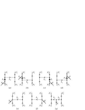
Figure 1: The two-body meson exchange currents in free-space. The thick lines in the diagrams (a) to (d) represent the $\Delta$ propagation.

The $\Delta$ current is derived from the Peccei pseudo-vector Lagrangian and reads

$$\bm{J}^{\mu}_{\Delta}(k_{1},k_{2}) = -\frac{1}{V^{2}}\frac{f_{\pi NN}f_{\pi N\Delta}f_{\gamma N\Delta}}{2M\mu_{\pi}^{2}}\left\{\left[\left(\frac{2}{3}\tau_{3}^{(2)}-\frac{i}{3}(\bm{\tau}^{(1)}\times\bm{\tau}^{(2)})_{3}\right)\left(j^{\mu}_{(a)}(p_{a},k_{2},q)\gamma_{5}\right)_{(1)}\right.\right.$$ (4)

$$+\left.\left.\left(\frac{2}{3}\tau_{3}^{(2)}+\frac{i}{3}(\bm{\tau}^{(1)}\times\bm{\tau}^{(2)})_{3}\right)\left(\gamma_{5}j^{\mu}_{(b)}(p_{b},k_{2},q)\right)_{(1)}\right]\Pi(k_{2})_{(2)}+(1\leftrightarrow 2)\right\}.$$

It corresponds to diagrams (a)-(d) of Fig. 1. In the above equations $M_{\Delta}$ denotes the isobar mass, $p_{a}\equiv p_{1}-q$, $p_{b}\equiv p_{1}^{\prime}+q$ and $f_{\pi N\Delta}=0.54$, $f_{\gamma N\Delta}=5$ yield the strength of the coupling of the $\Delta$ to the EM and pionic fields, respectively.

In Eq. (4) the following definitions have been introduced:

$$j_{(a)\mu}(p,k,q)=(4k_{\beta}-\hbox to0.0pt{/\hss}k\gamma_{\beta})S^{\beta\gamma}(p,M_{\Delta})\frac{1}{2}\left(-\gamma_{\mu}\hbox to0.0pt{/\hss}q\gamma_{\gamma}+q_{\mu}\gamma_{\gamma}\right)$$ (5a)

and

$$j_{(b)\mu}(p,k,q)=\frac{1}{2}\left(-\gamma_{\beta}\hbox to0.0pt{/\hss}q\gamma_{\mu}+q_{\mu}\gamma_{\beta}\right)S^{\beta\gamma}(p,M_{\Delta})(4k_{\gamma}-\gamma_{\gamma}\hbox to0.0pt{/\hss}k);$$ (5b)

the analogous expressions associated with the diagrams (c) and (d) are simply obtained through the interchange ($1\leftrightarrow 2$) as indicated in Eq. (4), which also implies $p_{a}\leftrightarrow p_{c}$ and $p_{b}\leftrightarrow p_{d}$ ($p_{c}\equiv p_{2}-q$, $p_{d}\equiv p_{2}^{\prime}+q$).

Furthermore, the Rarita-Schwinger (RS) $\Delta$ propagator, namely

$$S^{\beta\gamma}(p,M_{\Delta})=\frac{\gamma\cdot p+M_{\Delta}}{p^{2}-{M_{\Delta}}^{2}}\left(g^{\beta\gamma}-\frac{\gamma^{\beta}\gamma^{\gamma}}{3}-\frac{2p^{\beta}p^{\gamma}}{3{M_{\Delta}}^{2}}-\frac{\gamma^{\beta}p^{\gamma}-\gamma^{\gamma}p^{\beta}}{3M_{\Delta}}\right),$$ (6)

is used (we employ here the metric $a_{\mu}b^{\mu}=a^{0}b^{0}-\bm{a}\cdot\bm{b}$).

In the Appendix, the explicit expressions of Eqs. (5a-b) are reported.

The non-relativistic limit for the currents

The above given currents are the basic ingredients required in modeling $R_{T}$. Since one of our goals is to assess the quality of a given non-relativistic approximation for $R_{T}$, we also need the corresponding matrix elements of the currents in that limit. Under the assumption that the momenta of the nucleons involved in the response are small in comparison to their rest mass (which may or may not be valid) one obtains

$$J_{f}(\bm{k}_{1},\bm{k}_{2}) = -\frac{(2M)^{2}}{V^{2}}\frac{f_{\pi NN}^{2}f_{\gamma\pi\pi}}{\mu_{\pi}^{2}}4\tau_{1}\delta_{\tau_{1},-\tau_{2}}\delta_{\tau_{1}^{\prime},-\tau_{1}}\delta_{\tau_{2}^{\prime},-\tau_{2}}\frac{\chi^{\dagger}_{\sigma_{1}^{\prime}}\bm{\sigma}\cdot\bm{k}_{1}\chi_{\sigma_{1}}}{\bm{k}_{1}^{2}+\mu_{\pi}^{2}}\;\frac{\chi^{\dagger}_{\sigma_{2}^{\prime}}\bm{\sigma}\cdot\bm{k}_{2}\chi_{\sigma_{2}}}{\bm{k}_{2}^{2}+\mu_{\pi}^{2}}\bigl{(}\bm{k}_{2}-\bm{k}_{1}\bigr{)},$$

$$J_{s}(\bm{k}_{1},\bm{k}_{2}) = -\frac{(2M)^{2}}{V^{2}}\frac{f_{\pi NN}f_{\gamma\pi NN}}{\mu_{\pi}^{2}}4\tau_{1}\delta_{\tau_{1},-\tau_{2}}\delta_{\tau_{1}^{\prime},-\tau_{1}}\delta_{\tau_{2}^{\prime},-\tau_{2}}$$ (8)

$$\qquad\times\left[\chi^{\dagger}_{\sigma_{1}^{\prime}}\bm{\sigma}\chi_{\sigma_{1}}\frac{\chi^{\dagger}_{\sigma_{2}^{\prime}}\bm{\sigma}\cdot\bm{k}_{2}\chi_{\sigma_{2}}}{\bm{k}_{2}^{2}+\mu_{\pi}^{2}}-\frac{\chi^{\dagger}_{\sigma_{1}^{\prime}}\bm{\sigma}\cdot\bm{k}_{1}\chi_{\sigma_{1}}}{\bm{k}_{1}^{2}+\mu_{\pi}^{2}}\chi^{\dagger}_{\sigma_{2}^{\prime}}\bm{\sigma}\chi_{\sigma_{2}}\right]$$

and

$$J_{\Delta}(\bm{k}_{1},\bm{k}_{2}) = \frac{8Mf_{\pi NN}f_{\pi N\Delta}f_{\gamma N\Delta}}{3V^{2}\mu_{\pi}^{2}}\left\{\vphantom{\frac{\chi^{\dagger}_{\sigma}}{\bm{k}_{2}^{2}+\mu_{\pi}^{2}}}\left[\vphantom{\chi^{\dagger}_{\sigma_{1}^{\prime}}}iB\delta_{\tau_{1}^{\prime}\tau_{1}}\delta_{\tau_{2}^{\prime}\tau_{2}}\bigl{(}\bm{q}\times\bm{k}_{2}\bigr{)}\delta_{\sigma_{1}^{\prime}\sigma 1}\right.\right.$$

$$\left.\left.-A\delta_{\tau_{1},-\tau_{2}}\delta_{\tau_{1}^{\prime},-\tau_{1}}\delta_{\tau_{2}^{\prime},-\tau_{2}}\chi^{\dagger}_{\sigma_{1}^{\prime}}\bigl{[}\bm{q}\times(\bm{k}_{2}\times\bm{\sigma})\bigr{]}\chi_{\sigma_{1}}\right]\tau_{2}\frac{\chi^{\dagger}_{\sigma_{2}^{\prime}}\bm{\sigma}\cdot\bm{k}_{2}\chi_{\sigma_{2}}}{\bm{k}_{2}^{2}+\mu_{\pi}^{2}}+(1\leftrightarrow 2)\right\},$$

(9)

where

$$A=2\frac{2M_{\Delta}+M-\frac{\displaystyle 2M^{2}}{\displaystyle 3M_{\Delta}}+\frac{\displaystyle M^{3}}{\displaystyle 3M_{\Delta}^{2}}}{(M_{\Delta}^{2}-M^{2})}=2\frac{6M_{\Delta}^{2}-3MM_{\Delta}+M^{2}}{3M_{\Delta}^{2}(M_{\Delta}-M)}$$ (10a)

and

$$B=2\frac{2M_{\Delta}+3M+\frac{\displaystyle 2M^{2}}{\displaystyle 3M_{\Delta}}-\frac{\displaystyle M^{3}}{\displaystyle 3M_{\Delta}^{2}}}{(M_{\Delta}^{2}-M^{2})}=2\frac{6M_{\Delta}^{2}+3MM_{\Delta}-M^{2}}{3M_{\Delta}^{2}(M_{\Delta}-M)}.$$ (10b)

It should be noted, however, that this is not the only possible choice for a non-relativistic $\Delta$ current. For instance the one employed in Van80 and Alb84 indeed has the same structure as Eq. (9), but occurs with coefficients given by the following expressions

$$A=2\frac{(2M_{\Delta}+M)}{M_{\Delta}^{2}-M^{2}}\quad\quad\quad\text{and}\quad\quad\quad\ B=2\frac{(2M_{\Delta}+3M)}{M_{\Delta}^{2}-M^{2}},$$ (11)

which are obtained by disregarding the last two terms in the numerator of Eq. (10a-b). Note that these terms have opposite sign and affect the magnitude of the coefficients $A$ and $B$, in opposite direction, by less than 10%. The non-relativistic $\Delta$-current employed in DBT is again given by Eq. (9), however with coefficients

$$A=\frac{8}{3(M_{\Delta}-M)}\quad\quad\quad\quad\text{and}\quad\quad\quad\quad B=2A,$$ (12)

derived by setting $M=M_{\Delta}$ in the numerator of the right hand side of Eqs. (10a-b). The 2p-2h response function is stable with respect to these different definitions of the coefficients $A$ and $B$ (the changes amounting to a few percent).

III The response function

We turn now to the 2p-2h transverse response function, which can be obtained through the hadronic tensor. The latter is defined according to

$$W_{\mu\nu}(q^{2})=\frac{(2\pi)^{3}V}{4}\frac{V^{4}}{(2\pi)^{12}} \int\frac{d\bm{p}_{1}^{\prime}\,d\bm{p}_{2}^{\prime}\,d\bm{p}_{1}\,d\bm{p}_{2}}{16E_{\bm{p}_{1}^{\prime}}E_{\bm{p}_{2}^{\prime}}E_{\bm{p}_{1}}E_{\bm{p}_{2}}}\delta^{(4)}(q+p_{1}^{\prime}+p_{2}^{\prime}-p_{1}-p_{2})$$ (13)

$$\qquad\times\langle F|\bm{J}_{\mu}^{\dagger}|p_{1}^{\prime}p_{2}^{\prime}p_{1}p_{2}\rangle\langle p_{1}^{\prime}p_{2}^{\prime}p_{1}p_{2}|\bm{J}_{\nu}|F\rangle,$$

where $|F\rangle$ represents the Fermi sphere, $E_{\bm{p}}=\sqrt{\bm{p}^{2}+M^{2}}$, $\bm{J}\equiv\bm{J}_{\pi}+\bm{J}_{\Delta}=\bm{J}_{f}+\bm{J}_{s}+\bm{J}_{\Delta}$ and the factor 1/4 accounts for the identity of the 2 particles and 2 holes in the final states.

Being concerned with $R_{T}$ in the present work, actually we only need the spatial components of $W_{\mu\nu}$ (in fact only the $\mu=\nu=1$ and 2 components in the combination $11+22$, since the unpolarized transverse response is the focus). That is, we have

$$R_{T}(\bm{q},\omega) = \frac{(2\pi)^{3}V}{4}\frac{V^{4}}{(2\pi)^{12}}\int\frac{d\bm{p}_{1}^{\prime}\,d\bm{p}_{2}^{\prime}\,d\bm{p}_{1}\,d\bm{p}_{2}}{16E_{\bm{p}_{1}^{\prime}}E_{\bm{p}_{2}^{\prime}}E_{\bm{p}_{1}}E_{\bm{p}_{2}}}\theta(|\bm{p}_{1}^{\prime}|-k_{F})\theta(|\bm{p}_{2}^{\prime}|-k_{F})\theta(k_{F}-|\bm{p}_{1}|)$$ (14)

$$\times\theta(k_{F}-|\bm{p}_{2}|)\delta[\omega-(E_{\bm{p}_{1}^{\prime}}+E_{\bm{p}_{2}^{\prime}}-E_{\bm{p}_{1}}-E_{\bm{p}_{2}})]\delta^{(3)}(\bm{q}+\bm{p}_{1}^{\prime}+\bm{p}_{2}^{\prime}-\bm{p}_{1}-\bm{p}_{2})$$

$$\times 2\sum_{\sigma\tau}\sum_{i,j=1}^{3}\left(\delta_{ij}-\frac{q_{i}q_{j}}{\bm{q}^{2}}\right)\left[J_{i}^{\dagger}(\bm{p}_{1}^{\prime}-\bm{p}_{1},\bm{p}_{2}^{\prime}-\bm{p}_{2})J_{j}(\bm{p}_{1}^{\prime}-\bm{p}_{1},\bm{p}_{2}^{\prime}-\bm{p}_{2})\right.$$

$$\qquad\qquad\qquad\qquad\qquad\left.-J_{i}^{\dagger}(\bm{p}_{1}^{\prime}-\bm{p}_{1},\bm{p}_{2}^{\prime}-\bm{p}_{2})J_{j}(\bm{p}_{1}^{\prime}-\bm{p}_{2},\bm{p}_{2}^{\prime}-\bm{p}_{1})\right].$$

This expression explicitly displays the direct and exchange contribution stemming from the antisymmetrization of the 2p-2h final states in Eq. (13). In Eq. (14) the $J_{i}$ are the matrix elements of the currents in Eqs. (1), (2) and (4) in momentum space. Note that we define the excitation energy as $\omega=-q_{0}$.

By eliminating one of the integrations via the $\delta^{(3)}$, a simpler expression for the transverse response emerges:

$$R_{T}(\bm{q},\omega) = \frac{V}{2(2\pi)^{9}}\int{d\bm{p}_{1}^{\prime}\,d\bm{p}_{1}\,d\bm{p}_{2}}\theta(|\bm{p}_{1}^{\prime}|-k_{F})\theta(|\bm{p}_{2}^{\prime}|-k_{F})\theta(k_{F}-|\bm{p}_{1}|)\theta(k_{F}-|\bm{p}_{2}|)$$ (15)

$$\times\delta[\omega-(E_{\bm{p}_{1}^{\prime}}+E_{\bm{p}_{2}^{\prime}}-E_{\bm{p}_{1}}-E_{\bm{p}_{2}})]\sum_{\sigma\tau}\sum_{i,j=1}^{3}\frac{V^{4}}{16E_{\bm{p}_{1}^{\prime}}E_{\bm{p}_{2}^{\prime}}E_{\bm{p}_{1}}E_{\bm{p}_{2}}}\left(\delta_{ij}-\frac{q_{i}q_{j}}{\bm{q}^{2}}\right)$$

$$\times\left[J_{i}^{\dagger}(\bm{k}_{1},\bm{k}_{2})J_{j}(\bm{k}_{1},\bm{k}_{2})-J_{i}^{\dagger}(\bm{k}_{1},\bm{k}_{2})J_{j}(\bm{k}_{1}^{\prime},\bm{k}_{2}^{\prime})\right],$$

where now $\bm{p}_{2}^{\prime}=-\bm{q}+\bm{p}_{1}+\bm{p}_{2}-\bm{p}_{1}^{\prime}$. The exchange term in Eq. (15) depends on the pionic momenta $\bm{k}_{i}^{\prime}$ defined as $\bm{k}_{1}^{\prime}=\bm{p}_{1}^{\prime}-\bm{p}_{2}$, $\bm{k}_{2}^{\prime}=\bm{p}_{2}^{\prime}-\bm{p}_{1}$.

By exploiting the remaining $\delta$-function and with some algebra, the integral defining the transverse response can be reduced to seven dimensions. In previous work where only the direct term and the non-relativistic limit were considered, it turned out to be possible to reduce the integration to a bi-dimensional one; but now for the relativistic expression, this is no longer possible, even for the direct term.

As anticipated in the Introduction the traces of the relativistic currents typically generate a huge number of terms, so that it is not practical to report explicitly the expressions used in the numerical calculations of the relativistic responses. However, in the Appendix we give the formulae for the direct pion and pion/$\Delta$ contributions, the only ones having sizes suitable for publication.

Numerical integrations have been performed using Monte Carlo techniques, varying the sample size until a standard deviation better than 1% is reached. The number of configurations required for such an accuracy is $10^{6}\div 10^{7}$. A more stringent test of the accuracy in the numerical calculations can be obtained in the case of the direct non-relativistic contribution, since this can be reduced to a two-dimensional integral Van80 and done through standard quadrature. Also here the agreement is at the 1% level.

The non-relativistic limit

Before addressing the issue of the numerical evaluation of the fully relativistic problem, below we report the non-relativistic limit of the integrands in Eq. (15), to be referred to as ${\cal R}_{T}^{D}(\bm{k}_{1},\bm{k}_{2};\bm{q},\omega)$ and ${\cal R}_{T}^{E}(\bm{k}_{1},\bm{k}_{2};\bm{k}^{\prime}_{1},\bm{k}^{\prime}_{2};\bm{q},\omega)$, for the direct and exchange contributions, respectively. This will allow us to connect the various pieces contributing to the transverse response to specific Feynman diagrams and to ascertain from whence the major contributions arise. While the relativistic expressions for the transverse response function are quite cumbersome, the non-relativistic limit provides a relatively simple and controllable environment in which to check the correctness of the calculations. We also remark that our expression for ${\cal R}_{T}^{D}$ will turn out to differ somewhat from the one derived in DBT (no explicit formula is given there for the exchange part).

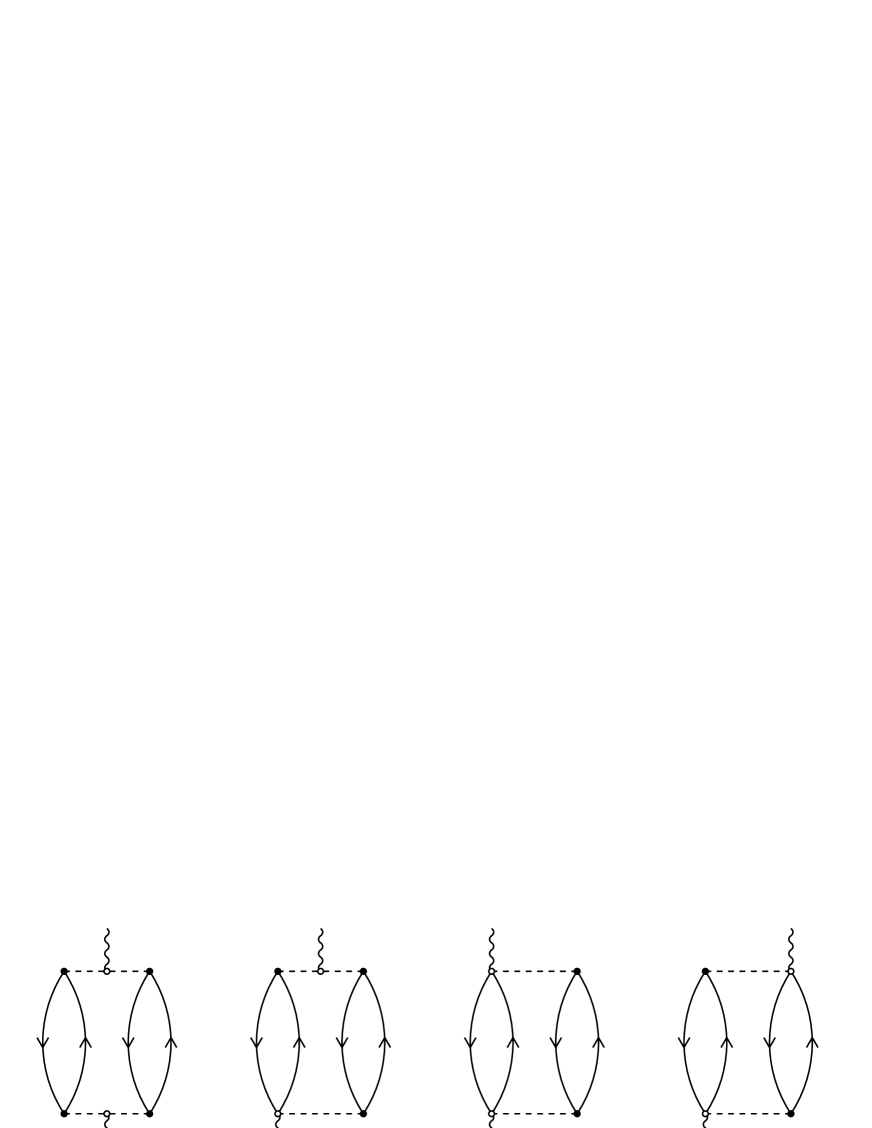
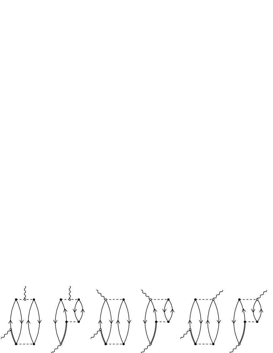
Figure 2: The direct pionic contributions to the MEC 2p-2h response function.

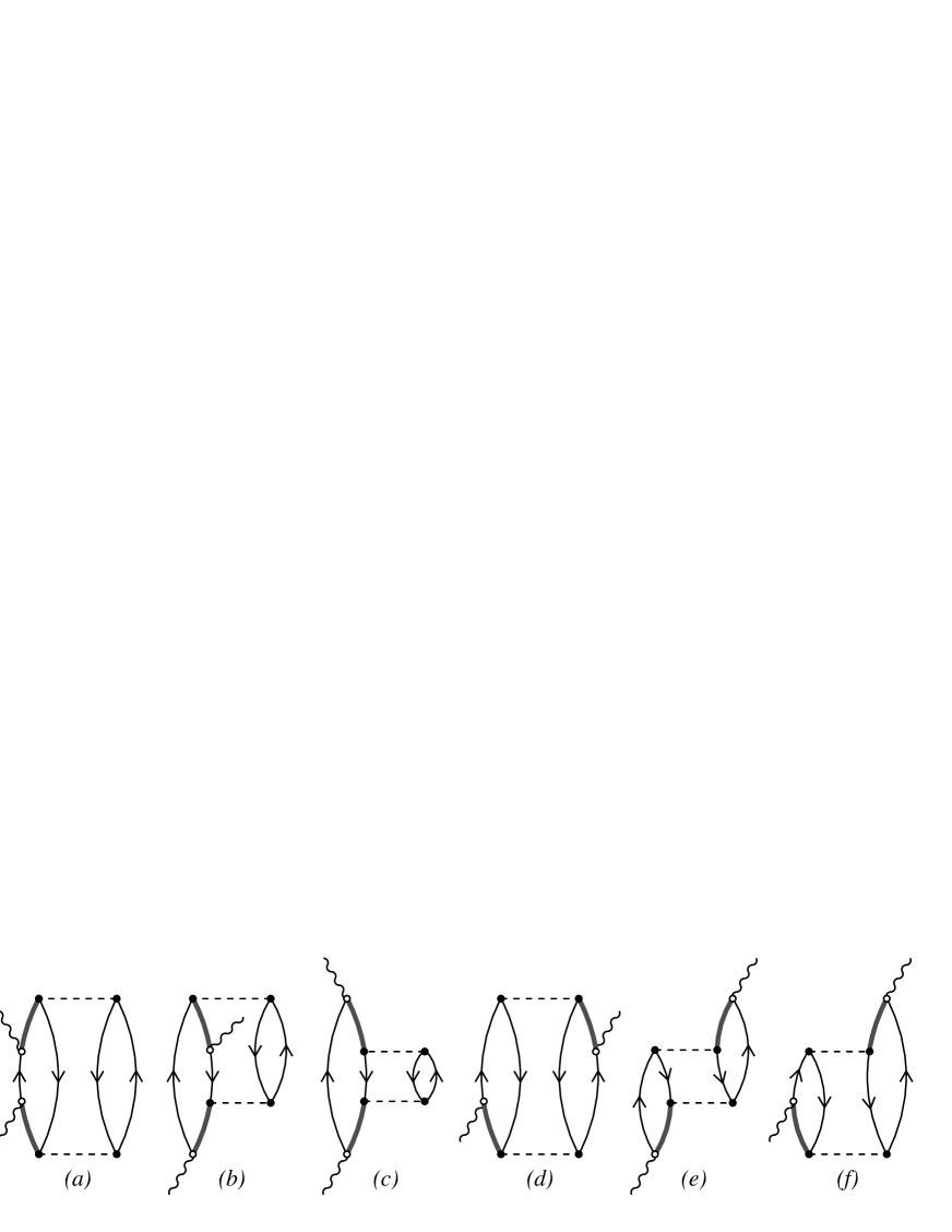
Figure 3: The direct pionic/$\Delta$ interference contributions to the MEC 2p-2h response function.

Figure 4: The direct $\Delta$ contributions to the MEC 2p-2h response function.

For the purely pionic contribution and for the interference between the pionic and $\Delta$ current we get, respectively,

$${\cal R}_{T}^{D\pi}(\bm{k}_{1},\bm{k}_{2};\bm{q},\omega) = \frac{V^{4}}{(2M)^{4}}\sum_{\sigma\tau}\sum_{ij}\left(\delta_{ij}-\frac{q_{i}q_{j}}{\bm{q}^{2}}\right)J_{i}^{\pi\dagger}(\bm{p}_{1}^{\prime}-\bm{p_{1}},\bm{p}_{2}^{\prime}-\bm{p}_{2})J_{j}^{\pi}(\bm{p}_{1}^{\prime}-\bm{p_{1}},\bm{p}_{2}^{\prime}-\bm{p}_{2})$$

$$= 128F^{2}_{\gamma NN}(q^{2})\left\{\frac{f_{\pi NN}^{4}f_{\gamma\pi\pi}^{2}}{\mu_{\pi}^{4}}\frac{\bm{k}_{1T}^{2}\,\bm{k}_{1}^{2}\bm{k}_{2}^{2}F_{\pi NN}^{2}(\bm{k}_{1}^{2})F_{\pi NN}^{2}(\bm{k}_{2}^{2})}{(\bm{k}_{1}^{2}+\mu_{\pi}^{2})^{2}(\bm{k}_{2}^{2}+\mu_{\pi}^{2})^{2}}\right.$$

$$\left.+\frac{f_{\pi NN}^{2}f_{\gamma\pi NN}^{2}}{2\mu_{\pi}^{4}}\left[\frac{\bm{k}_{1}^{2}F_{\pi NN}^{4}(\bm{k}_{1}^{2})}{(\bm{k}_{1}^{2}+\mu_{\pi}^{2})^{2}}+\frac{\bm{k}_{2}^{2}F_{\pi NN}^{4}(\bm{k}_{2}^{2})}{(\bm{k}_{2}^{2}+\mu_{\pi}^{2})^{2}}+\frac{(\bm{k}_{1T}\!\cdot\!\bm{k}_{2T})\,F_{\pi NN}^{2}(\bm{k}_{1}^{2})F_{\pi NN}^{2}(\bm{k}_{2}^{2})}{(\bm{k}_{1}^{2}+\mu_{\pi}^{2})(\bm{k}_{2}^{2}+\mu_{\pi}^{2})}\right]\right.$$

$$\left.-\frac{f_{\pi NN}^{3}f_{\gamma\pi NN}f_{\gamma\pi\pi}}{\mu_{\pi}^{4}}\left(\frac{\bm{k}_{1T}^{2}\bm{k}_{1}^{2}F_{\pi NN}^{3}(\bm{k}_{1}^{2})F_{\pi NN}(\bm{k}_{2}^{2})}{(\bm{k}_{1}^{2}+\mu_{\pi}^{2})^{2}(\bm{k}_{2}^{2}+\mu_{\pi}^{2})}+\frac{\bm{k}_{2T}^{2}\bm{k}_{2}^{2}F_{\pi NN}^{3}(\bm{k}_{2}^{2})F_{\pi NN}(\bm{k}_{1}^{2})}{(\bm{k}_{1}^{2}+\mu_{\pi}^{2})(\bm{k}_{2}^{2}+\mu_{\pi}^{2})^{2}}\right)\right\}$$

and

$${\cal R}_{T}^{D\{\pi\Delta\}}(\bm{k}_{1},\bm{k}_{2};\bm{q},\omega) = \frac{V^{4}}{(2M)^{4}}\sum_{\sigma\tau}\sum_{ij}\left(\delta_{ij}-\frac{q_{i}q_{j}}{\bm{q}^{2}}\right)$$

$$\times\Bigl{[}J_{i}^{\pi\dagger}(\bm{k}_{1},\bm{k}_{2})J_{j}^{\Delta}(\bm{k}_{1},\bm{k}_{2})+J_{i}^{\Delta\dagger}(\bm{k}_{1},\bm{k}_{2})J_{j}^{\pi}(\bm{k}_{1},\bm{k}_{2})\Bigr{]}$$

$$= 32A\frac{f_{\pi NN}^{2}f_{\pi N\Delta}f_{\gamma N\Delta}}{3\mu_{\pi}^{2}M}F_{\gamma NN}(q^{2})F_{\gamma N\Delta}(q^{2})$$

$$\times\left\{\frac{f_{\pi NN}f_{\gamma\pi\pi}}{\mu_{\pi}^{2}}F_{\pi NN}^{2}(\bm{k}_{1}^{2})F_{\pi NN}(\bm{k}_{2}^{2})F_{\pi N\Delta}(\bm{k}_{1}^{2})\frac{2\bm{q}^{2}\bm{k}_{1}^{2}\bm{k}_{1T}^{2}}{(\bm{k}_{1}^{2}+\mu_{\pi}^{2})^{2}(\bm{k}_{2}^{2}+\mu_{\pi}^{2})}\right.$$

$$+\frac{f_{\gamma\pi NN}}{\mu_{\pi}^{2}}\left[F_{\pi NN}^{3}(\bm{k}_{1}^{2})F_{\pi N\Delta}(\bm{k}_{1}^{2})\frac{2\bm{k}_{1}^{2}(\bm{k}_{1}\!\cdot\!\bm{q})}{(\bm{k}_{1}^{2}+\mu_{\pi}^{2})^{2}}\right.$$

$$\left.\left.+F_{\pi NN}^{2}(\bm{k}_{1}^{2})F_{\pi NN}(\bm{k}_{2}^{2})F_{\pi N\Delta}(\bm{k}_{2}^{2})\frac{\bm{q}^{2}\bm{k}_{1T}^{2}}{(\bm{k}_{1}^{2}+\mu_{\pi}^{2})(\bm{k}_{2}^{2}+\mu_{\pi}^{2})}\right]+(1\leftrightarrow 2)\right\}.$$

From the different coupling constants in Eqs. (III) and (III) it is easy to identify the contributions arising from the pion-in-flight and seagull currents. The topologically different diagrams are shown in Figs. 4 and 4.

Finally, for the contribution to ${\cal R}_{T}^{D}$ of the $\Delta$ current alone, one has

$${\cal R}_{T}^{D\Delta}(\bm{k}_{1},\bm{k}_{2};\bm{q},\omega) = \frac{V^{4}}{(2M)^{4}}\sum_{\sigma\tau}\sum_{ij}\left(\delta_{ij}-\frac{q_{i}q_{j}}{\bm{q}^{2}}\right)$$ (18)

$$\qquad\times{J}_{i}^{\Delta\dagger}(\bm{p}_{1}^{\prime}-\bm{p_{1}},\bm{p}_{2}^{\prime}-\bm{p}_{2}){J}_{j}^{\Delta}(\bm{p}_{1}^{\prime}-\bm{p_{1}},\bm{p}_{2}^{\prime}-\bm{p}_{2})$$

$$= \frac{8f_{\pi NN}^{2}f_{\pi N\Delta}^{2}f_{\gamma N\Delta}^{2}}{9M^{2}\mu_{\pi}^{4}}F_{\gamma N\Delta}^{2}(q^{2})\bm{q}^{2}$$

$$\qquad\times\left\{\left[F_{\pi NN}^{2}(\bm{k}_{1}^{2})F_{\pi N\Delta}^{2}(\bm{k}_{1}^{2})\left(B^{2}\frac{2\bm{k}_{1T}^{2}\bm{k}_{1}^{2}}{(\bm{k}_{1}^{2}+\mu_{\pi}^{2})^{2}}+A^{2}\frac{(\bm{k}_{1}^{2}+\bm{k}_{1L}^{2})\bm{k}_{1}^{2}}{(\bm{k}_{1}^{2}+\mu_{\pi}^{2})^{2}}\right)\right.\right.$$

$$\left.\left.\qquad+F_{\pi NN}(\bm{k}_{1}^{2})F_{\pi N\Delta}(\bm{k}_{1}^{2})F_{\pi NN}(\bm{k}_{2}^{2})F_{\pi N\Delta}(\bm{k}_{2}^{2})A^{2}\frac{\bm{k}_{1T}^{2}\bm{q}^{2}}{(\bm{k}_{1}^{2}+\mu_{\pi}^{2})(\bm{k}_{2}^{2}+\mu_{\pi}^{2})}\right]\right.$$

$$\left.\phantom{\frac{\bm{k}_{1T}^{2}\bm{q}^{2}}{(\bm{k}_{1}^{2}+\mu_{\pi}^{2})}}+(1\leftrightarrow 2)\right\},$$

where the first two terms on the right-hand side correspond to the diagrams (a)–(c) of Fig. 4, and the last one to the diagrams (d)–(f). In this case six distinct diagrams contribute.

In Eqs. (III), (III) and (18) $\bm{k}_{L}$ and $\bm{k}_{T}$ indicate the longitudinal and transverse components of the vector $\bm{k}$ with respect to the direction fixed by $\bm{q}$. Furthermore, in the appropriate places, the hadronic monopole form factors

$$F_{\pi NN}(k^{2}) = \frac{\Lambda_{\pi}^{2}-\mu_{\pi}^{2}}{\Lambda_{\pi}^{2}-k^{2}},$$ (19a)

$$F_{\pi N\Delta}(k^{2}) = \frac{\Lambda_{\pi N\Delta}^{2}}{\Lambda_{\pi N\Delta}^{2}-k^{2}}$$ (19b)

and the EM ones

$$F_{\gamma NN}(q^{2}) = \frac{1}{(1-q^{2}/\Lambda_{D}^{2})^{2}},$$ (19c)

$$F_{\gamma N\Delta}(q^{2}) = F_{\gamma NN}(q^{2})\left(1-\frac{q^{2}}{\Lambda_{2}^{2}}\right)^{-\frac{1}{2}}\left(1-\frac{q^{2}}{\Lambda_{3}^{2}}\right)^{-\frac{1}{2}}$$ (19d)

have been introduced. In the non-relativistic expressions the hadronic form factors have been taken in the static limit. The cut-offs have been chosen as in DBT, namely $\Lambda_{\pi}=1300$ MeV, $\Lambda_{\pi N\Delta}=1150$ MeV, $\Lambda_{D}^{2}=0.71$ GeV², $\Lambda_{2}=M+M_{\Delta}$ and $\Lambda_{3}^{2}=3.5$ GeV². This choice clearly makes it possible a direct comparison between our results for $R_{T}$ and those of DBT.

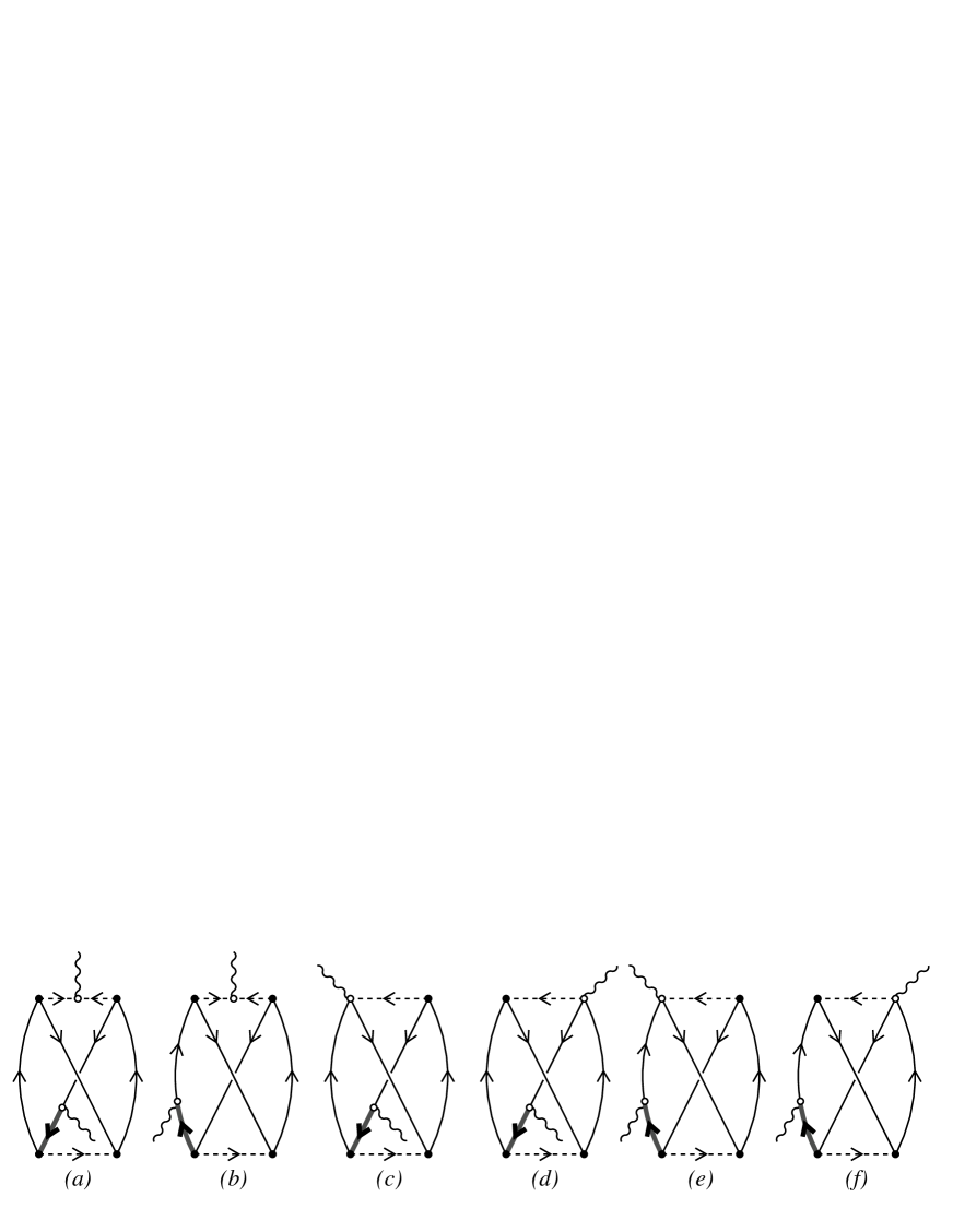
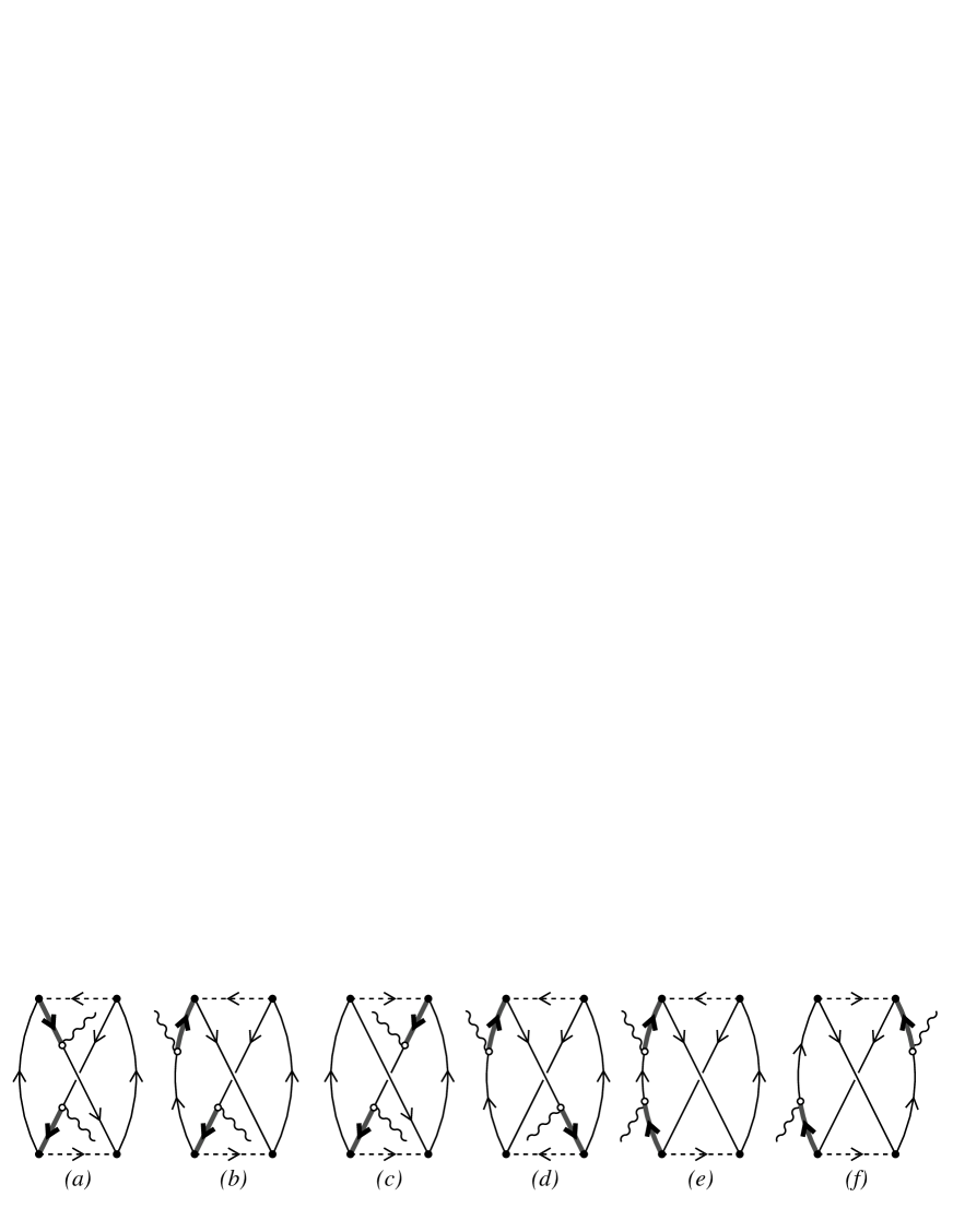
Figure 5: The exchange pionic/$\Delta$ interference contributions to the MEC 2p-2h response function.

Figure 6: The exchange $\Delta$ contributions to the MEC 2p-2h response function.

For completeness, we give also the formulae of the (smaller) exchange contributions to the integrand of Eq. (15), ${\cal R}_{T}^{E}(\bm{k}_{1},\bm{k}_{2};\bm{k}^{\prime}_{1},\bm{k}^{\prime}_{2};\bm{q},\omega)$, in the non-relativistic limit. The purely pionic contribution is identically zero, as a consequence of charge conservation and of the fact that the photon does not couple to a neutral pion. For the interference between pion and $\Delta$ (Fig. 6) we have

$${\cal R}_{T}^{E\{\pi\Delta\}}(\bm{k}_{1},\bm{k}_{2};\bm{k}_{1}^{\prime},\bm{k}_{2}^{\prime};\bm{q},\omega)=$$

$$=\frac{V^{4}}{(2M)^{4}}\sum_{\sigma\tau}\sum_{ij}\left(\delta_{ij}-\frac{q_{i}q_{j}}{\bm{q}^{2}}\right)\Bigl{[}J_{i}^{\pi\dagger}(\bm{k}_{1},\bm{k}_{2})J_{j}^{\Delta}(\bm{k}_{1}^{\prime},\bm{k}_{2}^{\prime})+J_{i}^{\Delta\dagger}(\bm{k}_{1},\bm{k}_{2})J_{j}^{\pi}(\bm{k}_{1}^{\prime},\bm{k}_{2}^{\prime})\Bigr{]}$$

$$=\frac{16f_{\pi NN}^{3}f_{\gamma\pi\pi}f_{\gamma N\Delta}f_{\pi N\Delta}}{3\mu_{\pi}^{4}M}B\bm{q}^{2}\left\{\frac{(\bm{k}_{2}\times\bm{k}_{2}^{\prime})_{L}^{2}}{(\bm{k}_{2}^{2}+\mu_{\pi}^{2})(\bm{k}_{2}^{\prime 2}+\mu_{\pi}^{2})}\left[\frac{1}{\bm{k}_{1}^{2}+\mu_{\pi}^{2}}+\frac{1}{\bm{k}_{1}^{\prime 2}+\mu_{\pi}^{2}}\right]+(1\leftrightarrow 2)\right\}$$

$$+\frac{8f_{\pi NN}^{3}f_{\gamma\pi NN}f_{\gamma N\Delta}f_{\pi N\Delta}}{3\mu_{\pi}^{4}M}B\left\{\frac{(\bm{q}\cdot\bm{k}_{2})\bm{k}_{2}^{\prime 2}+(\bm{q}\cdot\bm{k}_{2}^{\prime})\bm{k}_{2}^{2}-(\bm{q}\cdot\bm{k}_{2}^{\prime})(\bm{k}_{2}\cdot\bm{k}_{2}^{\prime})-(\bm{q}\cdot\bm{k}_{2})(\bm{k}_{2}\cdot\bm{k}_{2}^{\prime})}{(\bm{k}_{2}^{2}+\mu_{\pi}^{2})(\bm{k}_{2}^{\prime 2}+\mu_{\pi}^{2})}\right.$$

$$\qquad\left.+\frac{(\bm{q}\!\cdot\!\bm{k}_{1})\bm{k}_{2}^{\prime 2}-(\bm{q}\cdot\bm{k}_{2}^{\prime})(\bm{k}_{1}\cdot\bm{k}_{2}^{\prime})}{(\bm{k}_{1}^{2}+\mu_{\pi}^{2})(\bm{k}_{2}^{\prime 2}+\mu_{\pi}^{2})}+\frac{(\bm{q}\cdot\bm{k}_{1}^{\prime})\bm{k}_{2}^{2}-(\bm{q}\cdot\bm{k}_{2})(\bm{k}_{1}^{\prime}\cdot\bm{k}_{2})}{(\bm{k}_{1}^{\prime 2}+\mu_{\pi}^{2})(\bm{k}_{2}^{2}+\mu_{\pi}^{2})}+(1\leftrightarrow 2)\right\}.$$ (20)

The contribution of the $\Delta$ alone (Fig. 6) is instead

$${\cal R}_{T}^{E\Delta}(\bm{k}_{1},\bm{k}_{2};\bm{k}_{1}^{\prime},\bm{k}_{2}^{\prime};\bm{q},\omega)=\frac{V^{4}}{(2M)^{4}}\sum_{\sigma\tau}\sum_{ij}\left(\delta_{ij}-\frac{q_{i}q_{j}}{\bm{q}^{2}}\right)J_{i}^{\pi\dagger}(\bm{k}_{1},\bm{k}_{2})J_{j}^{\Delta}(\bm{k}_{1}^{\prime},\bm{k}_{2}^{\prime})$$ (21)

$$=\frac{4f_{\pi NN}^{2}f_{\pi N\Delta}^{2}f_{\gamma N\Delta}^{2}}{9M^{2}\mu_{\pi}^{4}}\bm{q}^{2}\left\{B^{2}\left[\frac{(\bm{k}_{1}\cdot\bm{k}_{1}^{\prime})(\bm{k}_{1T}\cdot\bm{k}_{1T}^{\prime})}{(\bm{k}_{1}^{2}+\mu_{\pi}^{2})(\bm{k}_{1}^{\prime 2}+\mu_{\pi}^{2})}+\frac{(\bm{k}_{1}\cdot\bm{k}_{2}^{\prime})(\bm{k}_{1T}\cdot\bm{k}_{2T}^{\prime})}{(\bm{k}_{1}^{2}+\mu_{\pi}^{2})(\bm{k}_{2}^{\prime 2}+\mu_{\pi}^{2})}+(1\leftrightarrow 2)\right]\right.$$

$$\left.\qquad\qquad+AB\left[\frac{2(\bm{k}_{1}\times\bm{k}_{1}^{\prime})_{L}^{2}-2k_{1L}k_{1L}^{\prime}(\bm{k}_{1}\cdot\bm{k}_{1}^{\prime})+k_{1L}^{\prime 2}\bm{k}_{1}^{2}+k_{1L}^{2}\bm{k}_{1}^{\prime 2}}{(\bm{k}_{1}^{2}+\mu_{\pi}^{2})(\bm{k}_{1}^{\prime 2}+\mu_{\pi}^{2})}\right.\right.$$

$$\left.\left.\qquad\qquad\qquad\qquad\frac{2(\bm{k}_{1}\times\bm{k}_{2}^{\prime})_{L}^{2}-2k_{1L}{k}_{2L}^{\prime}(\bm{k}_{1}\cdot\bm{k}_{2}^{\prime})+k_{2L}^{\prime 2}\bm{k}_{1}^{2}+k_{1L}^{2}\bm{k}_{2}^{\prime 2}}{(\bm{k}_{1}^{2}+\mu_{\pi}^{2})(\bm{k}_{2}^{\prime 2}+\mu_{\pi}^{2})}+(1\leftrightarrow 2)\right]\right\}.$$

Equations (III), (III) and (18) could in principle be compared with Eq. (5.11) of DBT; however, the overall normalization of the latter is not correct, since its dimension is not consistent with its definition (namely of being the transverse part of the amplitude ${\cal T}$ given in Eq. (4.8) of DBT); moreover, the relative weights of the interference and $\Delta$ contributions with respect to the pionic one differ, in our calculations, by a factor 2 and 4, respectively, from those of Eq. (5.11) of DBT. These factors, however, are not able to explain the marked difference between our results and those in that paper. Note that although the authors of DBT write down exactly the same expressions as we do for the non-relativistic MEC currents, actually they state that the non-relativistic procedure to get their Eq. (5.11) is applied at the level of the hadronic tensor, that is by reducing the (cumbersome) exact relativistic response.

In Fig. 7 we now compare our results with those of DBT, where the non-relativistic $R_{T}$ (without the exchange contribution) is shown for $q=550$ MeV/c (left) and for $q=1140$ MeV/c (right), with an atomic mass number of 56 and utilizing a Fermi momentum $k_{F}=1.3$ fm^-1. The latter value is employed for the sake of comparison with DBT, although in fact it is more appropriate for heavier nuclei.

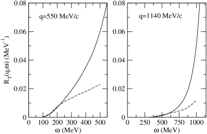
Figure 7: The non-relativistic transverse response function $R_{T}(q,\omega)$ according to the present calculation (solid) and to the one of DBT (dashed) for $q=550$ MeV/c and $q=1140$ MeV/c; in both instances $k_{F}=1.3$ fm^-1 and $\bar{\epsilon}_{2}=70$ MeV. Only the direct contribution is shown.

It is clearly apparent in the figure that our predictions differ significantly from those of DBT: while the discrepancy is mild for moderate values of $\omega$ (roughly, those encompassing the QEP), it becomes striking at higher energies, namely in the region of the so-called dip and of the $\Delta$-peak. Here our transverse response function in the proximity of the lightcone turns out to be larger by about a factor two at $q=550$ MeV/c and by over a factor three at $q=1140$ MeV/c.

Note that, in order to conform as closely as possible with the DBT approach, we have accounted for the initial state binding of the two holes by phenomenologically inserting a 70 MeV energy shift $\bar{\epsilon}_{2}$ in the energy conserving $\delta$-function appearing in the response function. In a non–relativistic framework this binding energy merely produces a shift of $R_{T}$ toward higher $\omega$ values. In the same spirit and to comply with gauge invariance, we have added (as in DBT) to the pion-in-flight current in Eq. (LABEL:eq:piinflight) two terms, to be viewed as the coupling of the virtual photon to a fictitious particle of mass equal to the $\pi NN$ cutoff, $\Lambda_{\pi}$, in spite of the very minor role these terms play in shaping the transverse response.

Furthermore, it is worth also remarking that our present calculations agree with the previous findings of  Van80 ; Alb84 . On the other hand, the computation of DBT does not agree with a previous one presented by the same authors in  Dek92 , notwithstanding that both of them employ the same set of values for the parameters and the kinematic conditions. Indeed, the former is lower than the latter by about 25%.

In the light of these new results, we anticipate contributions from MEC effects in the region beyond the QEP of a magnitude not previously foreseen in most previous work. Because the studies of  Van80 ; Alb84 were applied to moderate momenta and to a restricted range of transferred energies (not exceeding 300 MeV, in fact) owing to their non-relativistic nature, it is only in the studies of DBT that suggestions for such large effects can be found.

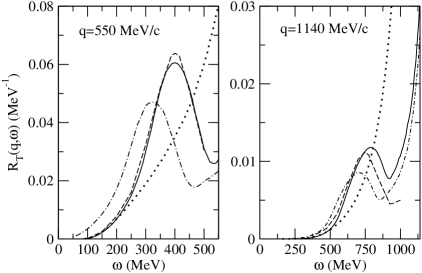
Figure 8: The relativistic transverse response function $R_{T}(q,\omega)$ at $q=550$ MeV/c and $q=1140$ MeV/c calculated with $\bar{\epsilon}_{2}=70$ MeV (solid) and with $\bar{\epsilon}_{2}=0$ (dot-dashed). Only the direct contribution is shown. The non-relativistic results are also displayed in order to shed light on the role of relativity in the response (dotted). For the sake of comparison the relativistic results obtained in DBT are displayed (dashed). In all instances $k_{F}=1.3$ fm^-1.

In the next section we shall explore whether or not the fully relativistic treatment and the inclusion of the exchange terms modify this finding.

IV Results in the relativistic regime

Direct Contributions

In Fig. 8 we display our relativistic results both without and with the energy shift $\bar{\epsilon}_{2}$, for the same conditions as those of Fig. 7. The exchange contribution is neglected here as well as in all the other figures of this subsection and considered separately below. In Fig. 8 we also compare our relativistic predictions both with those of DBT and with our non-relativistic results.

From the figure we observe the following.

a) The fully relativistic calculation differs considerably under some circumstances from the fully non-relativistic approximation (i. e., the solid and dotted curves in Fig. 8, respectively). Specifically relativity implies an increase of $R_{T}$ over the non-relativistic results in the region up to the $\Delta$ peak. Specifically, the overall effects are small in the domain of the QEP, are modest in the dip region and are substantial in the region of the $\Delta$-peak. In the region beyond the $\Delta$ peak, relativity instead yields a substantial reduction of the response with respect to the non-relativistic predictions. Of course, a hybrid approach can also be adopted in which spinor matrix elements and kinematics are kept non-relativistic, but the dynamic $\Delta$ propagator is used — this is discussed below.

b) The present relativistic and DBT relativistic calculations are in essential agreement at $q=550$ MeV/c and up to the $\Delta$ peak for $q=1140$ MeV/c.

c) In the dip following the $\Delta$ peak and above it up to the light cone, our transverse response is larger by about a factor two-to-three with respect to the DBT results.

d) At variance with the non-relativistic case, the binding energy not only shifts the relativistic $R_{T}$ toward higher energies, but also increases it.

e) Roughly speaking two effects are especially important in determining the characteristic behavior seen in Fig. 8. One is the peaking produced by the dynamic $\Delta$ propagation and the second is the basic phase space available to the two-nucleon ejection process. For instance, the strong rise of $R_{T}$ close to the light-cone at $q=1140$ MeV/c comes from the growth of the available phase space. We have checked this by setting all of the current matrix elements entering in Eq. (15) to unity and finding qualitatively the same behavior as in the full calculation.

To gain deeper insight into the transverse response, we display its individual contributions in Fig. 9 (for the non-relativistic case) and in Fig. 10 (for the relativistic one). In both instances the contribution of the $\Delta$ to $R_{T}$ is seen to be overwhelming (although this $\Delta$-dominance is mildly reduced by relativity), the more so at the larger momentum transfer. This feature strongly suggests the need for an appropriate treatment of the $\Delta$ degrees of freedom in obtaining EM responses over the whole kinematical regime under study. In particular the dynamical propagation of the latter appears to be essential, as discussed below. This in turn implies that a realistic accounting of the width of the $\Delta$ should be undertaken: here, again for ease of comparison with DBT, we have treated this problem as they did.

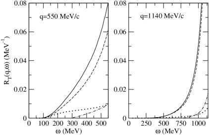
Figure 9: Separate contributions to the transverse response function $R_{T}(q,\omega)$ in the non-relativistic limit at $q=550$ MeV/c and $q=1140$ MeV/c: pionic (dotted), pionic-$\Delta$ interference (dash-dotted), $\Delta$ (dashed) and total (solid); $k_{F}=1.3$ fm^-1. The exchange contribution is disregarded here.

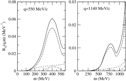
Figure 10: As in Fig. 9, but in the relativistic case.

Specifically, we have included the width through the replacement $M_{\Delta}\to M_{\Delta}-i\Gamma(s)/2$ in the energy denominator of Eq. (6), but not in the spinor factor. As far as $\Gamma(s)$ is concerned, $s$ being the square of the energy of the decaying $\Delta$ in its rest frame, we have adopted the same expression as in DBT.

To assess the crucial role played in $R_{T}$ by the $\Delta$ propagator more fully, in Fig. 11 we display the relativistic transverse response (hence computed with the dynamical $\Delta$ propagator) together with those obtained by neglecting the frequency dependence of $S^{\beta\gamma}(p,M_{\Delta})$ (the width of the $\Delta$ being neglected as well) in the two possible choices of a static ($p_{0}=0$) and of a constant $\Delta$ propagator. The extreme sensitivity of $R_{T}$ to $S^{\beta\gamma}(p,M_{\Delta})$ is clearly shown by the results in the figure.

One can understand even better the importance of treating correctly the $\Delta$ propagation by comparing the full relativistic results with a calculation employing the non-relativistic $\gamma N\Delta$ and $\pi N\Delta$ vertices, but retaining the relativistic, dynamical energy dependence in the denominator of the $\Delta$ propagator, $p^{2}-M_{\Delta}^{2}+iM_{\Delta}\Gamma$. In other words, one can invoke a hybrid model in which everything is kept non-relativistic, but where the dynamic dependence in the $\Delta$ propagator is retained. The results are mixed. If one wishes to study only the region extending through the peak seen in Fig. 11 out to the light-cone and wishes only to work at relatively small momentum transfers such as those in the figure, then this hybrid approach is reasonably good, incurring errors typically of $10\div 15\%$.

However, this is not a general statement. First, if one addresses higher $q$-values, much larger relativistic effects are apparent and the hybrid approach is not very successful. For instance, at $q=2$($3$) GeV/c the typical error made at the peak is $\approx 60(100)\%$. Secondly, if one focuses on the scaling region — as we shall in the follow-up study that is presently in progress — then even at relatively low values of $q$ the effects of relativity (i. e., effects other than the nature of the $\Delta$ propagator) are large. For instance, even at $q=1140$ MeV/c one finds effects exceeding 100% in the scaling region. This is not apparent in the figures presented here, since the cross sections are so small in that region. However, this does not mean that the scaling region is irrelevant — quite the opposite, the total cross section is also very small (but measurable) and the 2p-2h MEC effects are far from negligible. The details will be presented in the near future in a separate paper.

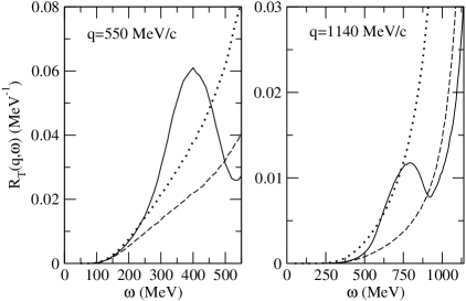
Figure 11: The relativistic transverse response function $R_{T}(q,\omega)$ at $q=550$ MeV/c and $q=1140$ MeV/c computed with various versions of the $\Delta$ propagator to illustrate the sensitivity to the latter: exact propagator (solid), static propagator (dashed) and constant propagator (dotted) (see text for the related definitions). In all instances $\bar{\epsilon}_{2}=70$ MeV and $k_{F}=1.3$ fm^-1.

Next let us comment on several general features that characterize the response in the 2p-2h sector in contradistinction with the 1p-1h case. In particular, the clean theoretical separation between the 1p-1h and the 2p-2h contributions holds only in the pure RFG framework. Here, moreover, the 1p-1h response is strictly confined to the well-known kinematical domain. In finite nuclei, or even in a correlated infinite Fermi system, neither of the above statements is valid any longer. We stick however to the pure RFG because this is the only model that allows us to maintain the fundamental principles of Lorentz covariance, gauge invariance and translational invariance.

The 2p-2h response function resides on the entire spacelike domain of the $(\omega,q)$-plane, in contrast to the 1p-1h case, which, as mentioned above, is constrained to a limited region — for recent fully relativistic studies of the 1p-1h response see Ama02 ; Ama02a ; Ama03 . Since momentum conservation involves only the total momentum there is no limitation on the momentum of a particle taking part in the 2p-2h excitations and hence the energy of the latter will vary over a broad range extending from $\omega=0$ to the light-cone.

In summary, naively the 2p-2h response function $R_{T}({q},\omega)$ might not be expected to display any particular structure, but rather to appear as a broad background. As a matter of fact, as we have seen, $R_{T}({q},\omega)$ indeed displays structure, but related not to the nuclear spectrum involved but to the role played by the $\Delta$ resonance. Furthermore, we have found that it grows with $\omega$, reflecting the associated growth of the phase space. Indeed the density per unit energy of the 2p-2h excitations goes as $\omega^{3}$.

Exchange Contributions

Considering the purely pionic MEC currents, it is well known Alb90 that the 1p-1h excited states of the RFG are reached only through the exchange term of the related MEC diagrams. In contrast the 2p-2h states are reached only through the direct term. The origin of these kinds of “selection rules” stems, in the first case, from the spin-isospin saturation of the RFG, in the second from the impossibility of fulfilling charge conservation in the exchange contribution for the diagrams displayed in Fig. 4.

The $\Delta$-current, however, eludes the above constraints. It provides a direct contribution in the 1p-1h sector of the RFG spectrum, as well as an exchange contribution in the 2p-2h sector, both alone and through the interference with the pionic currents.

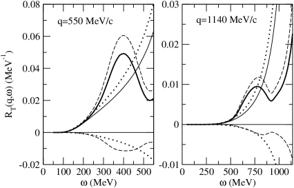
Figure 12: The transverse response function $R_{T}(q,\omega)$ at $q=550$ MeV/c and $q=1140$ MeV/c including the exchange contributions: non-relativistic direct (positive dotted), non-relativistic exchange (negative dotted), non-relativistic total (light solid), relativistic direct (positive dashed), relativistic exchange (negative dashed) and relativistic total (heavy solid). In all instances $\bar{\epsilon}_{2}=70$ MeV and $k_{F}=1.3$ fm^-1.

The exchange contributions are included together with the (larger) direct ones in Fig. 12. Two features are immediately apparent from the figure. First, the impact of relativity on the exchange terms is as substantial as it is for the direct ones. Moreover, as for the direct case, the exchange response is first enhanced in the region of the $\Delta$ and then dampened by the relativistic effects as one approaches the light cone.

Second, the relative magnitude of the exchange terms is seen to increase both with the energy transfer and with the momentum transfer. The fraction of the total relativistic response due to exchange goes from roughly 4% at low $\omega$ to 29% at the light cone for $q=550$ MeV/c and from 7% to 39% for $q=1140$ MeV/c. Thus, the exchange contribution, while not the dominant one in the kinematical situations we have explored, appears to us not only far from negligible, but also potentially interesting in connection with scaling (see below).

Finally, as for the direct case, note that the present calculation of the non-relativistic exchange contribution agrees with the calculation at lower momenta reported in  Van80 , whereas does not agree with that of DBT. The relativistic response, on the other hand, roughly agrees with DBT.

V Conclusions

In this paper we have carried out a fully relativistic calculation of the MEC contribution of 2p-2h excitations to the transverse inclusive response within the context of the RFG. These excitations are reached through the action of the MEC including the part associated with the $\Delta$ degrees of freedom. We have compared our results with those of DBT, the only existing relativistic study before the present one and we have pointed out similarities and differences between the two studies. To gauge the difficulty of this project it might help to stress again, as anticipated in the Introduction, that the number of terms we have computed to get $R_{T}$ amounts to over $100,000$.

Several new aspects contained in the present study bear highlighting. In particular, while the fully relativistic results obtained here roughly agree with those reported by DBT, some substantial differences occur, especially as the lightcone is approached. Furthermore, our non-relativistic results are completely in accord with our own previous work; however, they are not in agreement with DBT in many circumstances. Indeed, the strongest disagreements occur at high inelasticity and suggest to us that one should exercise extreme caution when invoking traditional non-relativistic approximations in such a regime.

Going beyond the extreme non-relativistic approximation Sch01 , one can invoke various classes of hybrid modeling where some, but not all, of the features of the fully relativistic model are retained Ryc01 ; Mac93 ; Bof91 . We have pursued such an approach in which the dynamic $\Delta$ propagator is kept, but otherwise everything is taken to be non-relativistic. The results are interesting: at modest $q$ (say 1 GeV/c or less) and at high $\omega$ the hybrid approach is quite good, incurring only $10\div 15\%$ error. However, at higher $q$-values, even in the high $\omega$ region, and at low $\omega$, even for modest $q$, the hybrid approach is not very successful and relativistic effects are important.

The high $\omega$ region, including the peak produced by the dynamic $\Delta$ propagator and the rise seen as the light-cone is approached when $q$ is large, might pose some problems for high-energy photoreactions. The latter are related in the familiar way (see, for example, DeF66 ) to the inclusive electron scattering transverse response by

$$\sigma^{\text{tot}}_{\gamma}=2\pi^{2}\frac{\alpha}{\omega}R_{T}(q,q),$$ (22)

$\alpha$ being the fine-structure constant.

In context, it is important to note that, while one cannot go from these results directly to studies of (e,e’NN) or ($\gamma$,NN) reactions (see, e. g., Refs. Car94 ; Ryc98 ; Giu01 ), since the RFG is not well-suited to modeling such semi-inclusive processes, the understanding gained in the present work concerning relativistic effects, $\Delta$ propagator effects, etc., likely can have an impact, for instance via improved descriptions of current operators for use in other approaches. The $\Delta$ propagator provides just one example: it produces a prominent peak in the 2p-2h transverse response and apparently is an important contribution in the total cross section. It is also very dependent on the specifics assumed, such as what model is taken for the propagator, how medium effects are or are not incorporated, how off-shellness is handled, etc. In particular, in view of continuing discussions about the off-shell behavior of the $\Delta$ inside the nuclear medium Pas98 and of our findings in this work, the 2p-2h transverse response may provide an ideal place in which to explore such issues.

Clearly, this is not the intent of the present work. Here we wish only to make contact with the work of DBT, using exactly their ingredients and only in future work will we return to address some of these interesting issues.

In particular, in the near future our intent is to address the difficult issue of the gauge invariance as was explored in the 1p-1h sector in  Ama02 ; Ama02a ; Ama03 . This requires the introduction of 2p-2h correlation currents in addition to the MEC. Only when this task is accomplished will a consistent (namely, gauge invariant), Lorentz covariant and translational invariant description of the inclusive responses (both longitudinal and transverse) within the RFG framework be achieved.

Furthermore, we are now in a position to study the degree to which these responses fulfill or violate $y$-scaling of first type (namely in the momentum transfer $q$) and of second type (namely in $k_{F}$) — see Don99 ; Don99a ; Mai02 . An exploration of these issues is currently being undertaken for the 2p-2h MEC and will be presented in a forthcoming paper, which will also focus on the important theme of the interplay between the scaling violations arising from the MEC action in both 1p-1h and 2p-2h sectors.

VI Acknowledgments

This work has been supported in part by the INFN-MIT Bruno Rossi Exchange Program and by MURST and in part (TWD) by funds provided by the U.S. Department of Energy under cooperative research agreement No. DE-DC02-94ER40818.

*

Appendix A

For completeness, in this appendix we report some of the detailed formulae used for the relativistic calculation.

We start by giving the explicit expressions for Eqs. (5a-b) which enter in the relativistic $\Delta$-current:

$$j_{(a)}^{\mu}(p,k,q) = \left\{\frac{1}{3M_{\Delta}^{2}}\Bigl{(}4\,(k\cdot p)\,p^{2}\,\gamma^{\mu}\hbox to0.0pt{/\hss}q-8\,(k\cdot p)\,(q\cdot p)\,\gamma^{\mu}\hbox to0.0pt{/\hss}{p}+8\,(k\cdot p)\,p_{\mu}\,\hbox to0.0pt{/\hss}q\hbox to0.0pt{/\hss}{p}\Bigr{.}\right.$$ (23a)

$$\Bigl{.}\;\;\;\;\;\;\;\;\;\;-p^{2}\hbox to0.0pt{/\hss}{k}\gamma^{\mu}\hbox to0.0pt{/\hss}q\hbox to0.0pt{/\hss}{p}-4\,q^{\mu}\,(k\cdot p)p^{2}\,{\bm{1}}+\,q^{\mu}\,p^{2}\,\hbox to0.0pt{/\hss}{k}\hbox to0.0pt{/\hss}{p}\Bigr{)}$$

$$+\frac{2}{3M_{\Delta}}\Bigl{(}4\,(k\cdot p)\,\gamma^{\mu}\hbox to0.0pt{/\hss}q\hbox to0.0pt{/\hss}{p}-p^{2}\,\hbox to0.0pt{/\hss}{k}\gamma^{\mu}\hbox to0.0pt{/\hss}q+2\,(q\cdot p)\,\hbox to0.0pt{/\hss}{k}\gamma^{\mu}\hbox to0.0pt{/\hss}{p}\Bigr{.}$$

$$\Bigl{.}\;\;\;\;\;\;\;\;\;\;-2\,p_{\mu}\,\hbox to0.0pt{/\hss}{k}\hbox to0.0pt{/\hss}q\hbox to0.0pt{/\hss}{p}-4\,(k\cdot p)\,q^{\mu}\,\hbox to0.0pt{/\hss}{p}+q^{\mu}\,p^{2}\,\hbox to0.0pt{/\hss}{k}\Bigr{)}$$

$$+\Bigl{(}\hbox to0.0pt{/\hss}{k}\gamma^{\mu}\hbox to0.0pt{/\hss}q\hbox to0.0pt{/\hss}{p}-2\,\hbox to0.0pt{/\hss}{p}\gamma^{\mu}\hbox to0.0pt{/\hss}q\hbox to0.0pt{/\hss}{k}-3\,q^{\mu}\,\hbox to0.0pt{/\hss}{k}\hbox to0.0pt{/\hss}{p}+4\,q^{\mu}\,(k\cdot p)\,{\bm{1}}\Bigr{)}$$

$$\left.+2M_{\Delta}\Bigl{(}-\gamma^{\mu}\hbox to0.0pt{/\hss}q\hbox to0.0pt{/\hss}{k}+q^{\mu}\,\hbox to0.0pt{/\hss}{k}\Bigr{)}\vphantom{\frac{1}{3M_{\Delta}^{2}}}\right\}\frac{1}{(p^{2}-M_{\Delta}^{2})},$$

$$j_{(b)}^{\mu}(p,k,q) = \gamma_{0}\Bigl{(}j_{(a)}^{\mu}(p,k,q)\Bigr{)}^{\dagger}\gamma_{0}$$ (23b)

Useful relations follow from momentum conservation: $q^{\mu}+k_{1}^{\mu}+k_{2}^{\mu}=0$, $\bm{k}_{1T}+\bm{k}_{2T}=0$ and $q=q_{L}=-k_{1L}-k_{2L}$. We also reiterate the definitions: $p_{a}\equiv p_{1}-q$, $p_{b}\equiv p_{1}^{\prime}+q$, $p_{c}\equiv p_{2}-q$, $p_{d}\equiv p_{2}^{\prime}+q$, $k_{i}\equiv p_{i}^{\prime}-p_{i}$.

Next, in the following formulae, we quote explicitly the integrand entering in the direct contributions to the transverse response, limiting ourselves to the full pionic contribution and to the pionic-$\Delta$ interference, since the pure $\Delta$ contribution corresponds to a far too lengthy expression to be reported here. We use the notation ${\cal E}\equiv E_{\bm{p}_{1}}E_{\bm{p}_{1}^{\prime}}E_{\bm{p}_{2}}E_{\bm{p}_{2}^{\prime}}$. The hadronic form factors are not explicitly displayed.

Pionic contribution:

$${\cal R}_{T}^{D\pi}(k_{1},k_{2};q) = \frac{V^{4}}{16{\cal E}}\sum_{\sigma\tau}\sum_{ij}\left(\delta_{ij}-\frac{q_{i}q_{j}}{\bm{q}^{2}}\right){J}_{i}^{\pi\dagger}(k_{1},k_{2}){J}_{j}^{\pi}(k_{1},k_{2})$$ (24)

$$= \frac{V^{4}}{16{\cal E}}\sum_{\sigma\tau}\sum_{m=x,y}{J}_{m}^{\pi\dagger}(k_{1},k_{2}){J}_{m}^{\pi}(k_{1},k_{2})$$

$$= 32\,\frac{M^{4}}{\mu_{\pi}^{4}{\cal E}}\,\left\{{f_{\pi NN}^{4}f_{\gamma\pi\pi}^{2}}\,\frac{4\bm{k}_{1T}^{2}\,k_{1}^{2}\,k_{2}^{2}\;}{(k_{1}^{2}-\mu_{\pi}^{2})^{2}(k_{2}^{2}-\mu_{\pi}^{2})^{2}}\right.$$

$$\left.+{f_{\pi NN}^{2}f_{\gamma\pi NN}^{2}}\,\left[\frac{2\,\bm{k}_{1T}^{2}}{(k_{1}^{2}-\mu_{\pi}^{2})(k_{2}^{2}-\mu_{\pi}^{2})}-\left(\frac{k_{1}^{2}(M^{2}+p_{20}p_{20}^{\prime}-p_{2L}p_{2L}^{\prime})}{M^{2}(k_{1}^{2}-\mu_{\pi}^{2})^{2}}+(1\leftrightarrow 2)\right)\right]\right.$$

$$\left.-{f_{\pi NN}^{3}f_{\gamma\pi NN}f_{\gamma\pi\pi}}\left[\frac{4\bm{k}_{1T}^{2}\,k_{1}^{2}}{(k_{1}^{2}-\mu_{\pi}^{2})^{2}(k_{2}^{2}-\mu_{\pi}^{2})}+(1\leftrightarrow 2)\right]\right\};$$

$\Delta$-pion interference contribution:

$${\cal R}_{T}^{D\{\Delta\pi\}}(k_{1},k_{2};q)=\frac{V^{4}}{16{\cal E}}\,\sum_{\sigma\tau}\sum_{m=x,y}\Bigl{[}{J}_{m}^{\Delta\dagger}(k_{1},k_{2}){J}_{m}^{\pi}(k_{1},k_{2})+{J}_{m}^{\pi\dagger}(k_{1},k_{2}){J}_{m}^{\Delta}(k_{1},k_{2})\Bigr{]}$$ (25)

$$= \frac{16M^{2}f_{\pi N\Delta}f_{\gamma N\Delta}}{3\mu_{\pi}^{4}{\cal E}}\left\{f_{\pi NN}^{3}f_{\gamma\pi\pi}\left[\frac{-k_{2}^{2}\sum\limits_{m}\Bigl{[}k_{1}^{m}\Bigl{(}{\mathcal{F}}_{a}^{m}(p_{1},p_{1}^{\prime};q)-{\mathcal{F}}_{b}^{m}(p_{1},p_{1}^{\prime};q)\Bigr{)}\Bigr{]}}{(k_{1}^{2}-\mu_{\pi}^{2})(k_{2}^{2}-\mu_{\pi}^{2})^{2}}+(1\leftrightarrow 2)\right]\right.$$

$$+ \left.f_{\pi NN}^{2}f_{\gamma\pi NN}\left[\vphantom{\frac{2M\sum\limits_{m}k_{2}^{m}\Bigl{(}\Bigr{)}}{(k_{1}^{2}-\mu_{\pi}^{2})}}\frac{k_{2}^{2}\Bigl{(}{\mathcal{S}}_{a}(p_{1},p_{1}^{\prime};q)+{\mathcal{S}}_{b}(p_{1},p_{1}^{\prime};q)\Bigr{)}}{4M(k_{2}^{2}-\mu_{\pi}^{2})^{2}}-\frac{\sum\limits_{m}k_{2}^{m}\Bigl{(}{\mathcal{F}}_{a}^{m}(p_{1},p_{1}^{\prime};q)+{\mathcal{F}}_{b}^{m}(p_{1},p_{1}^{\prime};q)\Bigr{)}}{2(k_{1}^{2}-\mu_{\pi}^{2})(k_{2}^{2}-\mu_{\pi}^{2})}\right.\right.$$

$$\left.\left.\hskip 341.43306pt+(1\leftrightarrow 2)\vphantom{\frac{\sum\limits_{m}k_{2}^{m}\Bigl{(}{\mathcal{F}}_{a}^{m}(p_{1},p_{1}^{\prime};q)\Bigr{)}}{2(k_{1}^{2}-\mu_{\pi}^{2})}}\right]\right\};$$

pure $\Delta$ contribution:

$${\cal R}_{T}^{D\Delta}(k_{1},k_{2};q) = \frac{V^{4}}{16{\cal E}}\sum_{\sigma\tau}\sum_{m=x,y}\left(J_{m}^{\Delta\dagger}(k_{1},k_{2})J_{m}^{\Delta}(k_{1},k_{2})\right)$$ (26)

$$= \frac{f_{\pi NN}^{2}f_{\pi N\Delta}^{2}f_{\gamma N\Delta}^{2}}{3\mu_{\pi}^{4}{\cal E}}\sum_{m=x,y}\left\{\left[\left(\vphantom{\frac{1}{1}}\frac{{\mathcal{F}}_{a}^{m}(p_{1},p_{1}^{\prime};q){\mathcal{F}}_{b}^{m}(p_{2},p_{2}^{\prime};q)}{3(k_{1}^{2}-\mu_{\pi}^{2})(k_{2}^{2}-\mu_{\pi}^{2})}\right.\right.\right.$$

$$+\frac{-k_{2}^{2}}{(k_{2}^{2}-\mu_{\pi}^{2})^{2}}\Bigl{[}\bm{Tr}\left\{(\hbox to0.0pt{/\hss}{p_{1}}-M)j_{(b)}^{m}(p_{a},k_{2},q)(\hbox to0.0pt{/\hss}{p_{1}}^{\prime}+M)j_{(a)}^{m}(p_{a},k_{2},q)\right\}$$

$$\hskip 71.13188pt+\bm{Tr}\left\{(\hbox to0.0pt{/\hss}{p_{1}}+M)j_{(a)}^{m}(p_{b},k_{2},q)(\hbox to0.0pt{/\hss}{p_{1}}^{\prime}-M)j_{(b)}^{m}(p_{b},k_{2},q)\right\}$$

$$\Bigl{.}\left.\left.-\frac{2}{3}\bm{Tr}\left\{(\hbox to0.0pt{/\hss}{p_{1}}+M)j_{(a)}^{m}(p_{b},k_{2},q)(\hbox to0.0pt{/\hss}{p_{1}}^{\prime}-M)j_{(a)}^{m}(-p_{a},k_{2},q)\right\}\Bigr{]}\right)+(1\leftrightarrow 2)\right]$$

$$\left.-\frac{{\mathcal{F}}_{a}^{m}(p_{1},p_{1}^{\prime};q){\mathcal{F}}_{a}^{m}(p_{2},p_{2}^{\prime};q)+{\mathcal{F}}_{b}^{m}(p_{1},p_{1}^{\prime};q){\mathcal{F}}_{b}^{m}(p_{2},p_{2}^{\prime};q)}{3(k_{1}^{2}-\mu_{\pi}^{2})(k_{2}^{2}-\mu_{\pi}^{2})}\right\}.$$

In the previous equations the following definitions have been introduced:

$${\mathcal{F}}_{a}^{m}(p,p^{\prime};q) \equiv \bm{Tr}\left\{(\hbox to0.0pt{/\hss}{p}-M)(\hbox to0.0pt{/\hss}{p}^{\prime}+M)j_{(a)}^{m}(p-q,-q-p^{\prime}+p,q)\right\}$$ (27f)

$$= \bm{Tr}\left\{(\hbox to0.0pt{/\hss}{p}-M)(\hbox to0.0pt{/\hss}{p}^{\prime}+M)j_{(a)}^{m}(p_{\Delta},k_{\pi},q)\right\}$$

$$= \frac{1}{p_{\Delta}^{2}-M_{\Delta}^{2}}\left\{\vphantom{\begin{array}[]{c}a\\ a\end{array}}\frac{4q^{2}}{3M_{\Delta}^{2}}\Bigl{[}p^{\prime m}(p\cdot q)-p^{m}(p^{\prime}\cdot q)+2p^{m}(p\cdot p^{\prime})\Bigr{]}\Bigl{[}p_{\Delta}^{2}-4(k_{\pi}\cdot p_{\Delta})\Bigr{]}\right.$$

$$+\frac{4M^{2}}{3M_{\Delta}^{2}}\left\{4(k_{\pi}\cdot p_{\Delta})\Bigl{[}p^{m}(p^{\prime}\cdot q)-p^{\prime m}(p\cdot q)+2p^{\prime m}q^{2}\Bigr{]}-q^{2}p_{\Delta}^{2}(p^{m}+p^{\prime m})\right\}$$

$$+\frac{8M}{3M_{\Delta}}\left\{k_{\pi}^{m}\Bigl{[}4(k_{\pi}\cdot p_{\Delta})(q\cdot p_{\Delta})-p_{\Delta}^{2}q^{2}+2(q\cdot p_{\Delta})^{2}\Bigr{]}\right.$$

$$\left.\hskip 42.67912pt-2p^{m}\Bigl{[}q^{2}(k_{\pi}\cdot p_{\Delta})+(k_{\pi}\cdot q)(q\cdotp_{\Delta})+2(k_{\pi}\cdot q)(k_{\pi}\cdot p_{\Delta})\Bigr{]}\right\}$$

$$+4\left\{q^{2}\Bigl{[}p^{\prime m}(q\cdot p)-p^{m}(q\cdot p^{\prime})\Bigr{]}+2(p\cdot p^{\prime})\Bigl{[}p^{m}q^{2}+2p^{m}(q\cdot p^{\prime})-2p^{\prime m}(q\cdot p_{\Delta})\Bigr{]}\right\}$$

$$\left.+4M^{2}\left\{4p^{\prime m}\Bigl{[}(q\cdot p_{\Delta})-p^{m}(p^{\prime}\cdot q)\Bigr{]}-q^{2}(p^{\prime m}+p^{m})\right\}+8MM_{\Delta}k_{\pi}^{m}q^{2}\vphantom{\begin{array}[]{c}a\\ a\end{array}}\right\},$$

$${\mathcal{F}}_{b}^{m}(p,p^{\prime};q) \equiv \bm{Tr}\left\{(\hbox to0.0pt{/\hss}{p}+M)(\hbox to0.0pt{/\hss}{p}^{\prime}-M)j_{(b)}^{m}(p^{\prime}+q,-q-p^{\prime}+p,q)\right\}$$ (27g)

$$= \bm{Tr}\left\{(\hbox to0.0pt{/\hss}{p}^{\prime}-M)(\hbox to0.0pt{/\hss}{p}+M)j_{(a)}^{m}(p^{\prime}+q,-q-p^{\prime}+p,q)\right\}={\mathcal{F}}_{a}^{m}(p^{\prime},p;-q).$$

$${\mathcal{S}}_{a}(p,p^{\prime};q) \equiv \sum_{m=x,y}\bm{Tr}\left\{(\hbox to0.0pt{/\hss}{p}-M)\gamma^{m}(\hbox to0.0pt{/\hss}{p}^{\prime}+M)j_{(a)}^{m}(p-q,-q-p^{\prime}+p,q)\right\}$$ (28f)

$$= \sum_{m=x,y}\bm{Tr}\left\{(\hbox to0.0pt{/\hss}{p}-M)\gamma^{m}(\hbox to0.0pt{/\hss}{p}^{\prime}+M)j_{(a)}^{m}(p_{\Delta},k_{\pi},q)\right\}$$

$$= \left\{\vphantom{\begin{array}[]{c}a\\ a\end{array}}\frac{8M}{3M_{\Delta}^{2}}\left\{4(k_{\pi}\cdot p_{\Delta})\Bigl{[}2(q\cdot p_{\Delta})\Bigl{(}(p^{\prime}\cdotp_{\Delta})-(q\cdot p1)\Bigr{)}-p_{\Delta}^{2}(q\cdot p1)\right.\right.\Bigr{.}$$

$$\left.\left.\Bigl{.}-\bm{p}_{T}^{2}\Bigl{(}q^{2}+(q\cdot pp1)\Bigr{)}+\bm{p}_{T}\cdot\bm{p}_{T}(q\cdot p_{\Delta})\Bigr{]}+p_{\Delta}^{2}\Bigl{[}q^{2}(k_{\pi}\cdot p)-(q\cdot k_{\pi})(p^{\prime}\cdot p_{\Delta})\right.\right.\Bigr{.}$$

$$\left.\Bigl{.}-3(q\cdot p^{\prime})(k_{\pi}\cdot p_{\Delta})-(q\cdot p_{\Delta})(k_{\pi}\cdot p^{\prime})+\bm{k}_{\pi T}\cdot\bm{p}_{T}\Bigl{(}q^{2}+(q\cdot p^{\prime})\Bigr{)}\right.$$

$$\left.-\bm{p}_{T}\cdot\bm{p}_{T}^{\prime}(q\cdot k_{\pi})\Bigr{]}\right\}+\frac{8M^{3}}{3M_{\Delta}^{2}}\Bigl{\{}8(q\cdot p_{\Delta})(k_{\pi}\cdot p_{\Delta})-p_{\Delta}^{2}(q\cdot k_{\pi})\Bigr{\}}$$

$$+\frac{16q^{2}}{3M_{\Delta}}\Bigl{\{}(q\cdot p^{\prime})(k_{\pi}\cdot p)-(q\cdot p)(k_{\pi}\cdot p^{\prime})-(q\cdot k_{\pi})(p\cdot p^{\prime})-4(p_{\Delta}\cdot k_{\pi})(p\cdot p^{\prime})\Bigr{.}$$

$$\Bigl{.}+\bm{p}_{T}\cdot\bm{p}_{T}^{\prime}\Bigl{[}p_{\Delta}^{2}-(p_{\Delta}\cdot k_{\pi})\Bigr{]}\Bigr{\}}+\frac{16M^{2}}{3M_{\Delta}}\Bigl{\{}(q\cdot k_{\pi})\Bigl{[}(p\cdot p^{\prime})+p_{\Delta}^{2}\Bigr{]}-(q\cdot p)(k_{\pi}\cdot p^{\prime})\Bigr{.}$$

$$\left.+2q^{2}(k_{\pi}\cdot p^{\prime})+3(q\cdot p^{\prime})(k_{\pi}\cdot p)-4(q\cdot p^{\prime})(k_{\pi}\cdot q)+2(q\cdot p_{\Delta})(k_{\pi}\cdot p_{\Delta})\right.$$

$$\left.-\bm{p}_{T}^{2}\Bigl{(}q^{2}+(q\cdot p^{\prime})\Bigr{)}+\bm{p}_{T}\cdot\bm{p}_{T}^{\prime}(q\cdot p_{\Delta})\Bigr{\}}+8M\Bigl{\{}q^{2}(k_{\pi}\cdot p)-(q\cdot k_{\pi})(p^{\prime}\cdot p_{\Delta})\right.\Bigr{.}$$

$$\Bigl{.}\left.+(q\cdot p^{\prime})(k_{\pi}\cdot p_{\Delta})-(q\cdot p_{\Delta})(k_{\pi}\cdot p^{\prime})+\bm{k}_{\pi T}\cdot\bm{p}_{T}(q\cdot p^{\prime})-2\bm{k}_{\pi T}\cdot\bm{p}_{T}^{\prime}(q\cdot p_{\Delta})\right.\Bigr{.}$$

$$\Bigl{.}\left.+\bm{p}_{T}^{2}\Bigl{[}q^{2}+2(q\cdot p^{\prime})\Bigr{]}-\bm{p}_{T}\cdot\bm{p}_{T}^{\prime}\Bigl{[}(q\cdot p)+(q\cdot p^{\prime})\Bigr{]}\Bigr{\}}-8M^{3}\Bigl{\{}(q\cdot k_{\pi})\Bigr{\}}\right.$$

$$\left.+16M_{\Delta}\Bigl{\{}(p\cdot p^{\prime})\Bigl{[}q^{2}+2(q\cdot p^{\prime})\Bigr{]}+\bm{p}_{T}\cdot\bm{p}_{T}^{\prime}\Bigl{[}q^{2}+(q\cdot p^{\prime})\Bigr{]}-\bm{p}_{T}^{\prime 2}(q\cdot p)\Bigr{\}}\right.$$

$$\left.+16M_{\Delta}M^{2}\Bigl{\{}q^{2}-2(q\cdot p)\Bigr{\}}\vphantom{\begin{array}[]{c}a\\ a\end{array}}\right\}\frac{1}{p_{\Delta}^{2}-M_{\Delta}^{2}}$$

and

$${\mathcal{S}}_{b}(p,p^{\prime};q) \equiv \sum_{m=x,y}\bm{Tr}\left\{(\hbox to0.0pt{/\hss}{p}+M)\gamma^{m}(\hbox to0.0pt{/\hss}{p}^{\prime}-M)j_{(b)}^{m}(p^{\prime}+q,-q-p^{\prime}+p,q)\right\}={\mathcal{S}}_{a}(p^{\prime},p;-q).$$

In Eqs. (27f) and (LABEL:eq:RDasdir) we used $p_{\Delta}=p-q$ and $k_{\pi}=-q-p^{\prime}+p$ to simplify the expressions. Eqs. (27g) and (28) are consequences of the identities: $j_{(a,b)}^{m}(p,k,q)=j_{(a,b)}^{m}(p,-k,-q)$ and Eq. (23b).

The traces indicated in Eq. (26) involve thousands of terms and are not included here.

From Eqs. (24)–(26) the non-relativistic limit of Eq. (III) can be obtained by assuming that all the nucleonic momenta are much smaller than the nucleon rest mass.

References

• (1) M.J. Dekker, P.J. Brussaard, and J.A. Tjon, Phys. Rev. C 49 (1994) 2650.
• (2) J.A.M. Vermaseren, New features of FORM, math-ph/0010025.
• (3) J.W. Van Orden and T.W. Donnelly, Ann. Phys. (N.Y.) 131 (1980) 451.
• (4) W.M. Alberico, M. Ericson, and A. Molinari, Ann. Phys. (N.Y.) 154 (1984) 356.
• (5) A. Gil, J. Nieves, E. Oset, Nucl. Phys. A 627 (1997) 543.
• (6) M.J. Dekker, P.J. Brussaard, and J.A. Tjon, Phys. Lett. B 289 (1992) 255.
• (7) J.E. Amaro, M.B. Barbaro, J.A. Caballero, T.W. Donnelly, and A. Molinari, Nucl. Phys. A 697 (2002) 388.
• (8) J.E. Amaro, M.B. Barbaro, J.A. Caballero, T.W. Donnelly, and A. Molinari, Phys. Rep. 368 (2002) 317.
• (9) J.E. Amaro, M.B. Barbaro, J.A. Caballero, T.W. Donnelly, and A. Molinari, (to be published in Nucl. Phys. A).
• (10) W.M. Alberico, T.W. Donnelly, and A. Molinari, Nucl. Phys. A 512 (1990) 541.
• (11) R. Schiavilla, in Nuclear Structure, edited by G.C. Bonsignori et al. (World Scientific, Singapore, 2001), nucl-th/0010061.
• (12) J. Ryckebusch, Phys. Rev. C 64 (2001) 044606.
• (13) L. Machenil, M. Vanderhaeghen, J. Ryckebusch, and M. Waroquier, Phys. Lett. B 316 (1993) 17.
• (14) S. Boffi and M.M. Giannini, Nucl. Phys. A 533 (1991) 441.
• (15) T. De Forest and J. D. Walecka, Adv. Phys. 15 (1966) 1.
• (16) R.C. Carrasco, M.J. Vicente Vacas and E. Oset, Nucl. Phys. A 570 (1994) 701.
• (17) J. Ryckebusch, D. Debruyne and W. Van Nespen, Phys. Rev. C 57 (1998) 1319.
• (18) C. Giusti and F.D. Pacati, Eur. Phys. J. A 12 (2001) 69.
• (19) V. Pascalutsa, Phys. Rev. D 58 (1998) 096002.
• (20) T.W. Donnelly and I. Sick, Phys. Rev. Lett. 82 (1999) 3212.
• (21) T.W. Donnelly and I. Sick, Phys. Rev. C 60 (1999) 065502.
• (22) C. Maieron, T.W. Donnelly and I. Sick, Phys. Rev. C 65 (2002) 025502.