Generator Coordinate Truncations

Abstract

We investigate the accuracy of several schemes to calculate ground-state correlation energies using the generator coordinate technique. Our test-bed for the study is the $sd$ interacting boson model, equivalent to a 6-level Lipkin-type model. We find that the simplified projection of a triaxial generator coordinate state using the $S_{3}$ subgroup of the rotation group is not very accurate in the parameter space of the Hamiltonian of interest. On the other hand, a full rotational projection of an axial generator coordinate state gives remarkable accuracy. We also discuss the validity of the simplified treatment using the extended Gaussian overlap approximation (top-GOA), and show that it works reasonably well when the number of boson is four or larger.

I INTRODUCTION

The self-consistent mean-field theories with a phenomenological nucleon-nucleon interaction have enjoyed a success in describing ground state properties of a wide range of atomic nuclei with only a few adjustable parameters (see Ref.[1] for a recent review). They are now at a stage where the ground state correlations beyond the mean-field approximation have to be taken into account seriously. This is partly due to the fact that much more accurate calculations have been increasingly required in recent years because of the experimental progress in the production of nuclei far from the stability line, where the ground state correlation beyond the mean-field approximation may play an important role. The major part of the correlations produces effects which have smooth trends with proton and neutron number. These are already incorporated into the energy functionals of effective mean-field models as, e.g., Skyrme-Hartree-Fock or the relativistic mean-field model. However, the correlations associated with low-energy modes show strong variations with shell structure, and cannot be contained in a smooth energy-density functional. This concerns the low-energy quadrupole vibrations and all zero-energy modes associated with symmetry restoration. In fact, the correlation effects appear most dramatically for these symmetry modes as there are: the center of mass localization, the rotational symmetry, and the particle number conservation. Those correlation effects must be taken into account explicietly in order to develop a global theory which can be extrapolated to the drip-line regions.

There are many ways that correlation energies can be calculated. In Ref. [2], we investigated a method which uses the random phase approximation (RPA). We found that the RPA provides a useful correlation around a spherical as well as for a well deformed configurations, but it fails badly around the phase transition point between spherical and deformed. Because of this defect, the RPA approach does not seem the best method for a global theory. Recently, we have developed an alternative method, called the top-GOA, to calculate the ground state correlation energies based on the generator coordinate method [3]. This is a generalization of the Gaussian Overlap Approximation (GOA) by taking into account properly the topology of the generator coordinate[4]. This method can be easily applied to the variation after projection (VAP) scheme, where the energy is minimized after the mean-field wave function is projected on to the eigenstates of the symmetry [5]. We have tested this method on the three-level Lipkin model, which consists of one vibrational degree of freedom and one rotational [3], and have confirmed that the method provides an efficient computational means to calculate ground state correlation energies for the full range of coupling strengths.

In this paper, we continue our study on the correlation energies using a model which contains the full degrees of freedom of quadrupole motion. To this end, we use a $sd$ interacting boson model (IBM)[6, 7], which may be viewed as a 6-level extension of the Lipkin model [8]. The IBM is particularly tailored for the description of the low-lying collective modes, thus provides a good testing ground for the present studies of correlations. In realistic systems, treating all the five quadrupole degrees of freedom is a difficult task in many aspects. Even if one restricts oneself to the rotational degrees of freedom, one in general has to deal with integrals over the three Euler angles, $\phi$, $\theta$, and $\chi$. The full triaxial projection is still too costly, since a number of rotated wave functions may be required in order to get a converged result. Also, the top-GOA scheme for triaxial nuclei is not as simple as in the three-level Lipkin model, because one has to take into account properly the coupling among the three Euler angles. How can one overcome these difficulties? We shall study here two approximate projection methods. One is the approximate angular momentum projection proposed by Bonche et al.[9], which uses the $S_{3}$ subgroup of the rotation group. With this approximation, one needs only five rotated wave functions. The other scheme which we consider is the axially symmetric approximation, where the energy is minimized with respect to the deformation $\beta$ only, setting the triaxiality $\gamma$ equal to zero. With this approximation, the integrations for the $\phi$ and $\chi$ angles become unnecessary, reducing the projection to a one-dimensional integral over $\theta$. The axially symmetric approximation has been widely used in the mean-field calculations [10, 11], where the approximation seems reasonable given that the most nuclei do not have a static triaxial ground state. However, it is not obvious whether the approximation remains valid when the fluctuations around the mean-field configuration are included, especially when the deformation is small.

The paper is organized as follows. In Sec. II, we set up the model Hamiltonian and discuss several approaches. These include the mean-field approximation, the full triaxial angular momentum projection and its approximation, the axially symmetric approximation, and the top-GOA for the axial projection. In Sec. III, we compare these schemes with the exact solutions of the Hamltonian obtained from the matrix diagonalization. We especially focus on the feasibility of each method in realistic systems. We then summarize the paper in Sec. IV.

II $sd$ boson Hamiltonian

Consider a $N$ boson system whose Hamiltonian is given by,

$$H=H_{0}+V=\epsilon\sum_{\mu}d_{\mu}^{\dagger}d_{\mu}-\frac{1}{2}\sum_{\mu}Q_{\mu}^{\dagger}Q_{\mu}.$$ (1)

The first term expresses the single-particle Hamiltonian $H_{0}$, while the second term is the residual quadrupole-quadrupole interaction. The quadrupole operator $Q_{\mu}$ is defined as

$$Q_{\mu}=\lambda_{1}(s^{\dagger}\tilde{d}_{\mu}+d_{\mu}^{\dagger}s)+\lambda_{2}[d^{\dagger}\tilde{d}]^{(2\mu)},$$ (2)

where $\tilde{d}_{\mu}=(-)^{\mu}\,d_{-\mu}$. When $\lambda_{1}=\lambda_{2}=0$ and $\epsilon>0$, the ground state is the $s$-boson condensed state, whose wave function is given by $(s^{\dagger})^{N}/\sqrt{N!}\,|\,\rangle$. For a finite value of $\lambda_{1}$ and $\lambda_{2}$, the Hamiltonian may be diagonalized using the number basis given by,

$$|\{n\}\rangle=|n_{s}\,n_{d_{-2}}\,n_{d_{-1}}\,n_{d_{0}}\,n_{d_{1}}\,n_{d_{2}}\rangle,$$ (3)

taking only the configurations satisfying

$$n_{s}+n_{d_{-2}}+n_{d_{-1}}+n_{d_{0}}+n_{d_{1}}+n_{d_{2}} = N,$$ (4)

$$-2n_{d_{-2}}-n_{d_{-1}}+n_{d_{1}}+2n_{d_{2}} = 0.$$ (5)

The first condition, (4), constrains the boson number, while the second equation, (5), is the condition that the $z$ component of the angular momentum is zero. With these constraints, the basis has a dimenion of 5 for $N=2$, 18 for $N=4$, and 203 for $N=10$. We are going to compare the exact solutions obtained in this way with results of the collective treatment based on the mean-field approximation plus angular momentum projection.

A Mean-field approximation

We first solve the Hamiltonian in the mean-field approximation. To this end, we consider an intrinsic deformed mean-field state given by [7]

$$|\beta\gamma\rangle=\frac{1}{\sqrt{N!}}(b^{\dagger})^{N}\,|\,\rangle,$$ (6)

where the deformed boson operator is defined as

$$b^{\dagger}=\frac{1}{\sqrt{1+\beta^{2}}}\left(s^{\dagger}+\beta\cos\gamma\,d_{0}^{\dagger}+\frac{\beta}{\sqrt{2}}\sin\gamma\,(d_{2}^{\dagger}+d_{-2}^{\dagger})\right).$$ (7)

The parameter $\beta$ accoutns for the global deformation and $\gamma$ for triaxiality. The deformation energy surface then reads [7]

$$E_{\rm MF}(\beta,\gamma) = \langle\beta\gamma|H|\beta\gamma\rangle,$$ (8)

$$= \epsilon\,\frac{N\beta^{2}}{1+\beta^{2}}$$ (11)

$$-\frac{1}{2}\,\frac{N}{(1+\beta^{2})^{2}}\,\lambda_{1}^{2}\left\{(1+\beta^{2})\left(5+\left(1+\frac{\lambda_{2}^{2}}{\lambda_{1}^{2}}\right)\beta^{2}\right)\right.$$

$$\left.+(N-1)\left(4\beta^{2}-\sqrt{\frac{32}{7}}\,\frac{\lambda_{2}}{\lambda_{1}}\,\beta^{3}\cos 3\gamma+\frac{2}{7}\,\frac{\lambda_{2}^{2}}{\lambda_{1}^{2}}\,\beta^{4}\right)\right\}.$$

One finds that the energy minimum appears on the prolate side ($\beta>0,\gamma=0$) when $\lambda_{2}/\lambda_{1}<0$, while it is on the oblate side ($\beta>0,\gamma=\pi/3$) for $\lambda_{2}/\lambda_{1}>0$. When $\lambda_{2}$ is zero, the energy surface is independent of $\gamma$, corresponding to the $\gamma$-unstable case.

B Triaxial Angular Momentum Projection

When $\beta$ is non-zero, the intrinsic wave function (6) is not an eigenstate of the total angular momentum $J$. One can project this state onto the $J=0$ state as [5]

$$|\beta\gamma,J=0\rangle\propto\int d\Omega\,\hat{R}(\Omega)\,|\beta\gamma\rangle=\int^{2\pi}_{0}d\phi\int^{2\pi}_{0}d\chi\int^{\pi}_{0}\sin\theta d\theta\,\hat{R}(\phi,\theta,\chi)\,|\beta\gamma\rangle,$$ (12)

where $\hat{R}(\Omega)$ is the rotation operator. The corresponding energy is given by

$$E_{\rm proj}(\beta,\gamma)=\frac{\int d\Omega\,\langle\beta\gamma|H\hat{R}(\Omega)|\beta\gamma\rangle}{\int d\Omega\,\langle\beta\gamma|\hat{R}(\Omega)|\beta\gamma\rangle}.$$ (13)

Notice that the rotated wave function can be expressed in terms of the rotated boson operator as

$$|\beta\gamma\Omega\rangle\equiv\hat{R}(\Omega)\,|\beta\gamma\rangle=\frac{1}{\sqrt{N!}}(b_{R}^{\dagger})^{N}\,|\,\rangle,$$ (14)

with

$$b_{R}^{\dagger}\equiv\hat{R}(\Omega)b^{\dagger}\hat{R}^{-1}(\Omega) = \frac{1}{\sqrt{1+\beta^{2}}}\left(s^{\dagger}+\beta\cos\gamma\,\sum_{m}D^{2}_{m0}(\Omega)d_{m}^{\dagger}\right.$$ (16)

$$\left.+\frac{\beta}{\sqrt{2}}\sin\gamma\,\sum_{m}\left(D^{2}_{m2}(\Omega)+D^{2}_{m\,-2}(\Omega)\right)\,d_{m}^{\dagger}\right),$$

where $D^{2}_{mm^{\prime}}(\Omega)$ is the Wigner’s $D$ function. The overlaps in the projected energy (13) can be expressed in terms of commutators such as

$$[b,b_{R}^{\dagger}] = \frac{1}{1+\beta^{2}}\left(1+\beta^{2}\cos^{2}\gamma\,d^{2}_{00}(\theta)+\beta^{2}\sin^{2}\gamma\,[d^{2}_{22}(\theta)\cos(2\phi+2\chi)+d^{2}_{2-2}(\theta)\cos(2\phi-2\chi)]\right.$$ (18)

$$\left.\hskip 51.21504pt+\sqrt{2}\beta^{2}\sin\gamma\cos\gamma\,d^{2}_{20}(\theta)\,[\cos(2\chi)+\cos(2\phi)]\right).$$

The results are

$$I(\Omega) \equiv \langle\beta\gamma|\hat{R}(\Omega)|\beta\gamma\rangle=[b,b_{R}^{\dagger}]^{N},$$ (19)

$$\frac{H_{0}(\Omega)}{I(\Omega)} \equiv \frac{\langle\beta\gamma|H_{0}\hat{R}(\Omega)|\beta\gamma\rangle}{\langle\beta\gamma|\hat{R}(\Omega)|\beta\gamma\rangle}=\epsilon N\left(1-\frac{1}{[b,b_{R}^{\dagger}]}\right),$$ (20)

$$\frac{V(\Omega)}{I(\Omega)} \equiv \frac{\langle\beta\gamma|V\hat{R}(\Omega)|\beta\gamma\rangle}{\langle\beta\gamma|\hat{R}(\Omega)|\beta\gamma\rangle}=-\frac{N}{2}\,\frac{1}{[b,b^{\dagger}_{R}]}\,\sum_{m}\left[[b,Q_{m}^{\dagger}],[Q_{m},b_{R}^{\dagger}]\right]$$ (22)

$$\hskip 128.0374pt-{N(N-1)\over 2[b,b^{\dagger}_{R}]^{2}}\sum_{m}\left[b,[Q_{m},b_{R}^{\dagger}]\right]\left[[b,Q_{m}^{\dagger}],b_{R}^{\dagger}\right].$$

Here, we have used the relation

$$[\hat{A},\hat{B}^{N}]=N\hat{B}^{N-1}[\hat{A},\hat{B}]+\frac{1}{2}N(N-1)\hat{B}^{N-2}\,[[\hat{A},\hat{B}],\hat{B}]+\cdots,$$ (23)

for arbitrary operators $\hat{A}$ and $\hat{B}$. We give an explicit expression for the quadrupole commutators, $[Q_{m},b_{R}^{\dagger}]$ and $[Q_{m},b^{\dagger}]$, in the Appendix.

In practice, one can evaluate the integrals in Eq. (13) as follows. First notice that the integration intervals for the $\chi$ and $\phi$ angles can be reduced from $(0,2\pi)$ to $(0,\pi)$ since the $K$ quantum number is even for the intrinsic state (6) [12]. Next, because of the reflection symmetry of the intrinsic wave function (6) with respect to the $z$ plane, the integration range for the $\theta$ angle can be reduced to $(0,\pi/2)$. One can then apply the Gauss-Legendre quadrature formula to the $\theta$ integral, and the Gauss-Chebyschev formula to the $\chi$ and $\phi$ integrals [12, 13]. One may also try the simpler Simpson formula. We will check the convergence of these formulas in the next section.

C Approximate Triaxial Projection with Octahedral Group

Bonche et al. have considered an approximation to the triaxial angular momentum projection (12) based on the octahedral rotation group, that is a group formed from permutations of the principal axes of inertia [9]. With this representation, the projected wave function (12) is approximated as

$$|\beta\gamma,J=0\rangle\approx\sum_{i=1}^{24}\hat{S}_{i}|\beta\gamma\rangle,$$ (24)

where $\hat{S}_{i}$ are the 24 elements of the octahedral group. In our case with states even under parity, the octahedral group is reduced to $S_{3}$, the group of permutations of three objects (the $x,y,z$ axes). The 6 rotations to be treated are [9],

$$\hat{S}_{1} = \hat{R}(0,0,0)=1,$$ (25)

$$\hat{S}_{2} = \hat{R}(\pi,\pi/2,0),$$ (26)

$$\hat{S}_{3} = \hat{R}(-\pi/2,-\pi/2,0),$$ (27)

$$\hat{S}_{4} = \hat{R}(\pi/2,-\pi/2,\pi/2),$$ (28)

$$\hat{S}_{5} = \hat{R}(0,\pi,\pi/2),$$ (29)

$$\hat{S}_{6} = \hat{R}(0,\pi,-\pi/2).$$ (30)

D Axial Projection

When the triaxiality $\gamma$ is zero, the $\phi$ and $\chi$ integrals in Eq. (12) become trivial. The triple integral is then reduced to a much simpler single integral with respect to the angle $\theta$. This simplifies the projected energy (13) to

$$E_{\rm proj}(\beta)=\frac{\int^{1}_{-1}\,d(\cos\theta)\,(H_{0}(\theta)+V(\theta))}{\int^{1}_{-1}\,d(\cos\theta)\,I(\theta)},$$ (31)

where the overlaps in this axial approximation read

$$I(\theta) = \frac{1}{(1+\beta^{2})^{N}}\left(1+\frac{\beta^{2}}{2}(2-3\sin^{2}\theta)\right)^{N},$$ (32)

$$\frac{H_{0}(\theta)}{I(\theta)} = \epsilon N\cdot\frac{\beta^{2}(1-\frac{3}{2}\sin^{2}\theta)}{1+\beta^{2}(1-\frac{3}{2}\sin^{2}\theta)},$$ (33)

$$\frac{V(\theta)}{I(\theta)} = -\frac{N}{2}\cdot\frac{1}{[1+\beta^{2}(1-\frac{3}{2}\sin^{2}\theta)]^{2}}\,$$ (37)

$$\times\left\{\left(1+\beta^{2}(1-\frac{3}{2}\sin^{2}\theta)\right)\left(5\lambda_{1}^{2}+(\lambda_{1}^{2}+\lambda_{2}^{2})\beta^{2}(1-\frac{3}{2}\sin^{2}\theta)\right)\right.$$

$$\left.+(N-1)\beta^{2}\left(\lambda_{1}^{2}(1+3\cos^{2}\theta)+\frac{4}{\sqrt{14}}\lambda_{1}\lambda_{2}\beta(1-3\cos^{2}\theta)\right.\right.$$

$$\hskip 156.49014pt\left.\left.+\frac{\lambda_{2}^{2}}{14}\beta^{2}(4-9\sin^{2}\theta\cos^{2}\theta)\right)\right\}.$$

The axiallay projected energy (31) depends, of course, only on the global deformation $\beta$. VAP means then to minimize the projected energy with respect to the deformation parameter $\beta$.

E Top-GOA for Axial Projection

A further simplification may be achieved using a second-order approach, the extended Gaussian Overlap Approximation (top-GOA). In this scheme, the overlaps are expanded up to second order derivatives with respect to the generator coordinate while retaining its topology. For the axial projection considered in the previous subsection, the procedure is very similar as in Ref. [3] for the three-level Lipkin model. From Eqs. (32 – 37), it is clear that a natural choice for the expansion variable is $\sin\theta$. Expanding the overlaps with respect to $\sin\theta$, one obtains

$$I(\theta) \approx \exp\left(-\frac{3}{2}\,\frac{N\beta^{2}}{1+\beta^{2}}\sin^{2}\theta\right),$$ (38)

$$\frac{H_{0}(\theta)+V(\theta)}{I(\theta)} \approx E_{\rm MF}(\beta)+\frac{H_{2}(\beta)}{2}\sin^{2}\theta,$$ (39)

where $E_{\rm MF}(\beta)$ is the mean-field energy given by Eq. (11) (with $\gamma=0$), and $H_{2}(\beta)$ is defined as

$$H_{2}(\beta)=\left.\frac{d^{2}}{d\theta^{2}}\,\frac{H_{0}(\theta)+V(\theta)}{I(\theta)}\right|_{\theta=0}.$$ (40)

Note that we have exponentiated the normalization overlap $I(\theta)$ following the idea of the Gaussian overlap approximation [14].

III Numerical Results

A Comparison of projection schemes

The exact ground state for the model Hamiltonian (1) and the various integrals needed for the projection schemes are solved numerically by standard methods. Figure 1 compares the exact solution of the Hamiltonian with the several approximations to the triaxial angular momentum projection for $N$=4 and $\epsilon=1$. The interaction strength $\lambda_{2}$ is set to be $\lambda_{2}/\lambda_{1}=-\sqrt{7}/4$ for each $\lambda_{1}$, that is a half the SU(3) value, $(\lambda_{2}/\lambda_{1})_{\rm SU(3)}=-\sqrt{7}/2$ [15, 16]. The top panel of the figure shows the ground state correlation energy, i.e., a difference between the ground state and the mean-field energies, as a function of the interaction strength $\lambda_{1}$. The mean-field energy is obtained by minimizing the energy surface (11). The optimum deformation parameter $\beta$ thus obtained is shown by the thin solid line in the middle panel. One sees the phase transition between the spherical and the deformed configurations at $\lambda_{1}=0.47$. The results of full triaxial angular momentum projection, obtained by minimizing the projected energy surface (13), are shown by the solid circles in the top panel. These results reproduce well the exact results, indicating that the vibrational contribution is not large in this model. The optimum deformations $\beta$ and $\gamma$ are shown by the thick solid line in the middle and the bottom panels, respectively. In contrast to the mean-field approximation, the optimum deformation $\beta$ is finite for all the values of $\lambda_{1}$, showing no phase transition [3]. This is a well-known feature of the variation after projection (VAP) scheme [5]. The dotted line in the figure denotes the results of the approximate triaxial angular momentum projection by the $S_{3}$ subgroup of the rotation group. This method does not seem to provide enough correlation energy, and the agreement with the exact results is poor for all the region of $\lambda_{1}$.

What is the role played by the triaxiality $\gamma$ in these calculations? In order to study this, we show the results of full axial projection by the dashed line in the figure. These are obtained by minimizing the energy function (31), which is equivalent to minimizing (13) while keeping $\gamma=$0. We find that this approximation reproduces the exact solution remarkably well. The result might appear surprising, since the axially symmetric approximation is not expected to work near spherical, where all the five quadrupole degrees of freedom should contribute in a similar way. However, as we have already discussed, the VAP scheme always leads to a well developed deformation even when the mean-field configuration is spherical (see the middle panel), and such “dangerous” region can be avoided. Moreover, even though the optimum deformation can be small when the interaction strength is very small, this is an irrelevant case since the correlation effect is small there. Figure 2 shows the projected energy surface $E_{\rm proj}(\beta,\gamma)$, measured with respect to the energy of the pure configuration, $s^{4}$, at $\lambda_{1}=0.5$ and $\beta$=0.741 as a function of triaxiality $\gamma$. One sees that the energy gain due to the triaxial deformation is indeed small, being consistent with the performance of the axially symmetric approximation shown in fig.1. We summarize the results for $\lambda_{1}=0.5$ in Table I.

As a further test of the axially symmetric approximation, we repeat the calculations for $\lambda_{2}/\lambda_{1}=0$, that is the $\gamma$ unstable case. The results are shown in fig. 3, where the meaning of each line is the same as in fig. 1. Note that the optimum triaixiality parameter $\gamma$ in the triaxial angular momentum projection is 30 degree for all the values of $\lambda_{1}$, reflecting the $\gamma$ unstable nature of the mean-field approximation. In this case, the performance of the axial approximation is not as good as in fig.1 (see the dashed line). However, it still provides about 80% of correlation energy at $\lambda_{1}$ =1, and slightly larger at smaller values of $\lambda_{1}$, which may be acceptable even in realistic systems.

We notice here that the axially symmetric approximation is sufficient for $N=2$ irrespective of the value of $\lambda_{1}$ and $\lambda_{2}$. From Eqs. (12) and (14), the (normalized) wave function for $J=0$ state reads

$$|\beta\gamma,J=0\rangle=\frac{1}{\sqrt{2+\frac{2}{5}\,\beta^{4}}}\left.\left.\left[\sqrt{2}\,\frac{s^{\dagger}s^{\dagger}}{\sqrt{2}}+\frac{\beta^{2}}{5}\left(2\,d_{2}^{\dagger}d_{-2}^{\dagger}-2\,d_{1}^{\dagger}d_{-1}^{\dagger}+\sqrt{2}\,\frac{d_{0}^{\dagger}d_{0}^{\dagger}}{\sqrt{2}}\right)\right]\,\right|\,\right\rangle,$$ (41)

for any value of $\gamma$. The projected wave function is thus independent of $\gamma$, and so is the projected energy surface. We also note that the axially symmetric approximation becomes exact in the limit of $N\to\infty$, as was argued by Kuyucak and Morrison using the $1/N$ expansion technique [17]. For $N=2$, the wave function (41) is in fact exact, when $\beta$ is minimized. This follows from the observation there are only two $J=0$ states in the $(sd)^{4}$ configuration space, and their relative amplitudes can be set by a suitable choice of $\beta$, in case of attractive interactions. We have checked the trend in between the two limits, $N=2$ and large $N$. The influence of triaxiality are found strongest around $N=4$, where the correlation effects are also largest. The effect of triaxiality then decreases slowly as the boson number $N$ increases.

B Efficient angular momentum projection

We next discuss the feasibility of the angular momentum projection. From a computational point of view, it is a costly operation to apply the rotation operator to a mean-field configuration and take overlaps with it. Thus one wants to minimize the number of points in the angular integration mesh. Figure 4 shows the convergence of the angular integrals in the projected energy surface (13) with respect to the number of rotated wave functions $N_{\rm rot}$, for the same parameter set as in fig. 2. Notice that the relations $[H,P_{J}]=0$ and $(P_{J})^{2}=P_{J}$ are used in deriving Eq. (13), where $P_{J}$ is the projection operator. For a finite value of $N_{\rm rot}$, these relations may be violated, and consequently, the numerical formula does not give an upper bound of the energy. The open circles are the results of the Simpson method, while the closed circles are obtained with the Gaussian quadrature formulas (see Sec. II-C). These are for fixed values of deformation parameters $\beta$ and $\gamma$, as indicated in the inset of the figure. The upper panel is for the axial projection, while the lower panel for the triaxial projection. Note that the former is plotted as a function of $N_{\rm rot}$, while the latter involves the three integrals and is plotted as a function of $(N_{\rm rot})^{1/3}$. For the Simpson method, we exclude the $(\phi,\theta,\chi)=(0,0,0)$ point in counting the number of state $N_{\rm rot}$ in the horizontal axis. This state corresponds to the unrotated state from which the rotated wave functions are constructed, regardless of which quadrature formula one uses. The figure also shows the result of top-GOA and the approximate triaxial projection with the $S_{3}$ group as a comparison, which correspond to $N_{\rm rot}=1$ and 5, respectively. From the figure, one observes that the convergence for the axial projection is quick if one uses the Gauss-Legendre quadrature formula. The energy is almost converged at $N_{\rm rot}$ = 3. The Simpson method, on the other hand, requires more terms to achieve the convergence. For the triaxial projection, a similar convergence is seen for each of the three integrals. However, the required number of rotated wave functions is as large as 27 in total, making the triaxial angular momentum projection with the VAP minimization impractical. The situation is even worse for a larger value of $N$. To demonstrate this, figure 5 shows the results for $N=10$. The convergence is somewhat slower in this system compared with the $N=4$ case. Note that the $N_{\rm rot}$ points-Gauss-Legendre formula is exact when the maximum spin in the intrinsic state is $J_{\rm max}=2N_{\rm rot}-2$ [12, 18]. In the present $sd$ model, the maximum spin $J_{\rm max}$ is given by $2N$, and therefore the more points are needed in order to get a convergence for the larger value of $N$.

Lastly, we discuss the applicability of the top-GOA approach to axial projection (see Sec. II-E). This approach requires only one slightly rotated wave function in order to evaluate the second derivatives. Figure 6 shows the correlation energy for $N=4$ obtained with the top-GOA approximation (the dotted line), and with the full axial projection (the dashed line). The figure also contains the exact solutions as a comparison. The upper panel is for $\lambda_{2}/\lambda_{1}=-\sqrt{7}/4$, while the lower panel is for $\lambda_{2}/\lambda_{1}=0$. We see that the top-GOA approximation reproduces the full projection reasonably well. The performance is somewhat better for $\lambda_{2}/\lambda_{1}=-\sqrt{7}/4$. As was discussed in Ref. [3], the applicability of the top-GOA approaches increases quickly for a larger value of boson number $N$. Indeed, the upper panel of figs. 4 and 5 indicates that the agreement between the top-GOA and the exact projection significantly improves when $N$=10.

IV Summary

We have used the $sd$-interacting boson model to investigate projections in a generator coordinate approach to calculate the ground state correlation energy associated with the quadrupole motion. Our conclusions about the efficiency of various approximations are clear. The full angular momentum projection of a triaxial intrinsic state requires a large number of rotated wave functions, and it is too costly for realistic calculations. On the other hand, we found that the angular momentum projection of an axial intrinsic state provides a useful ground state correlation energy. The axially symmetric approximation is exact for $N=2$ and $N=\infty$. The number of rotated wave functions needed there is order of 4 if one uses the Gauss-Legendre quadrature formula to compute the angle integral. The approximate triaxial projection using the $S_{3}$ group requires 5 rotated wave functions and still performs rather poorly. We thus conclude that the axial projection provides the most promising method to compute systematically the ground state correlation energy for deformation.

In applying any projection or generator coordinate expansion, however, one has to bear in mind that up to now the energy density functional is defined for a single Slater determinant state. It is not designed for a multi-determinantal wave function such as the projected state, and there are ambiguities in calculating the density-dependent interaction energy using the energy functional. Although several recipes have been proposed, they are all subject to a conceptional problem. This difficulty can be avoided in either the following ways. One is to use the top-GOA approximation, which can be formulated in terms of the expectation values in the mean-field wave function [3]. We have studied the applicability of the top-GOA with the present model, and have shown that it already gives a reasonable result for $N=4$ and the performance improves for larger values of $N$. Alternatively, one may also specify the density-dependence in more detail to remove ambiguities. Along these lines, a new form of the Skyrme interaction was recently proposed by Duguet and Bonche [19]. In either way, the axially symmetric approximation leads to a substantial simplification to perform the angular momentum projection with only a few Slater determinants, providing a useful means to construct a microscopic global theory for the nuclear binding energy systematics.

A Quadrupole commutators

In this Appendix, we give an explicit expression for the quadrupole commutators, $[Q_{m},b_{R}^{\dagger}]$ and $[Q_{m},b^{\dagger}]$, in Eq. (22). For this purpose, it is convenient to use a compact notation for the boson operator, $b_{lm}$, where $b_{00}=s$ and $b_{2m}=d_{m}$. Using this notation, we express the quadrupole operator $Q_{m}$ and the rotated boson operator $b_{R}^{\dagger}$ as

$$Q_{m}=\sum_{l_{1},m_{1}}\sum_{l_{2},m_{2}}q^{(m)}_{l_{1}m_{1},l_{2}m_{2}}b_{l_{1}m_{1}}^{\dagger}b_{l_{2}m_{2}},$$ (A1)

and

$$b_{R}^{\dagger}=\sum_{l,m}B_{lm}(\Omega)\,b_{lm}^{\dagger},$$ (A2)

respectively. Here, the coefficients $q^{(m)}_{l_{1}m_{1},l_{2}m_{2}}$ and $B_{lm}(\Omega)$ are given by,

$$q^{(m)}_{00,2m_{1}} = (-)^{m}\lambda_{1}\,\delta_{m_{1},-m},$$ (A3)

$$q^{(m)}_{2m_{1},00} = \lambda_{1}\,\delta_{m_{1},m},$$ (A4)

$$q^{(m)}_{2m_{1},2m_{2}} = (-)^{m_{2}}\langle 2\,m_{1}\,2\,-m_{2}|2\,m\rangle\,\lambda_{2},$$ (A5)

$$B_{00}(\Omega) = \frac{1}{\sqrt{1+\beta^{2}}}\,,$$ (A6)

$$B_{2m}(\Omega) = \frac{1}{\sqrt{1+\beta^{2}}}\left(\beta\cos\gamma\,D^{2}_{m0}(\Omega)+\frac{\beta}{\sqrt{2}}\sin\gamma\,\left(D^{2}_{m2}(\Omega)+D^{2}_{m\,-2}(\Omega)\right)\right).$$ (A7)

From Eqs. (A1) and (A2), one finds

$$[Q_{m},b_{R}^{\dagger}]=\sum_{l_{1},m_{1}}\sum_{l_{2},m_{2}}q^{(m)}_{l_{1}m_{1},l_{2}m_{2}}B_{l_{2}m_{2}}(\Omega)\,b_{l_{1}m_{1}}^{\dagger}.$$ (A8)

The commutator $[Q_{m},b^{\dagger}]$ can be obtained by setting $\Omega=0$ in Eq. (A8). This yields,

$$\left[[b,Q_{m}^{\dagger}],[Q_{m},b_{R}^{\dagger}]\right] = \sum_{l_{1},m_{1}}\sum_{l_{2},m_{2}}\sum_{l_{3},m_{3}}q^{(m)}_{l_{1}m_{1},l_{2}m_{2}}q^{(m)}_{l_{1}m_{1},l_{3}m_{3}}B_{l_{2}m_{2}}(\Omega)B_{l_{3}m_{3}}(0),$$ (A9)

$$\left[b,[Q_{m},b_{R}^{\dagger}]\right] = \sum_{l_{1},m_{1}}\sum_{l_{2},m_{2}}q^{(m)}_{l_{1}m_{1},l_{2}m_{2}}B_{l_{2}m_{2}}(\Omega)B_{l_{1}m_{1}}(0),$$ (A10)

$$\left[[b,Q_{m}^{\dagger}],b_{R}^{\dagger}\right] = \sum_{l_{1},m_{1}}\sum_{l_{2},m_{2}}q^{(m)}_{l_{1}m_{1},l_{2}m_{2}}B_{l_{1}m_{1}}(\Omega)B_{l_{2}m_{2}}(0).$$ (A11)

TABLE I.: Comparison of the ground state energy $E$ and the optimum deformation parameters $\beta$ and $\gamma$ obtained with several methods. The parameters of the Hamiltonian are taken to be $N=4$, $\epsilon=1$, $\lambda_{1}=0.5$, and $\lambda_{2}/\lambda_{1}=-\sqrt{7}/4$. The energy is measured with respect to that of the pure configuration, $s^{4}$.

Scheme	$E-E(s^{4})$	$\beta$	$\gamma$ (deg.)
Exact	$-$0.8193	–	–
Triaxial Projection	$-$0.8189	0.741	17.64
Axial Projection	$-$0.8017	0.723	0.0

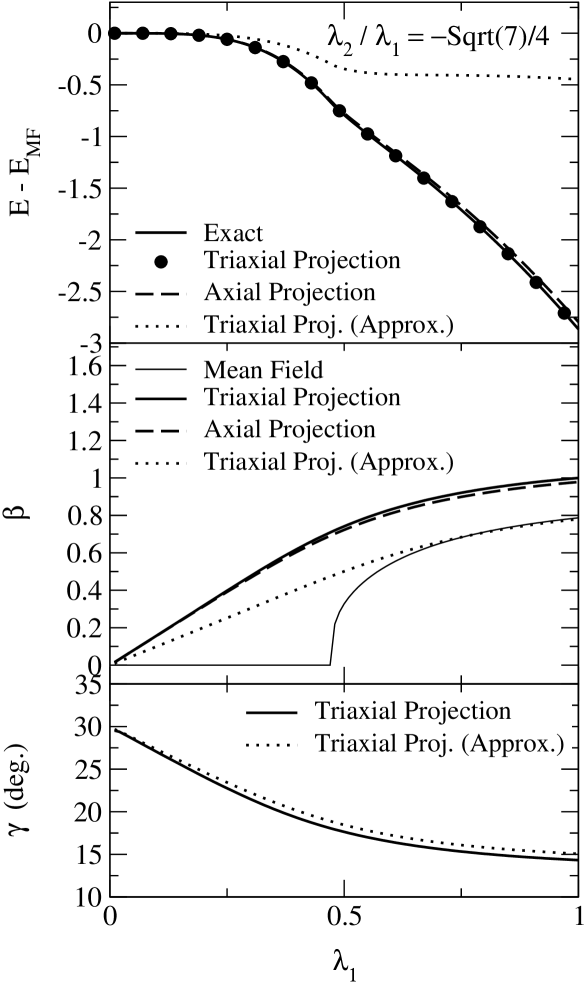
FIG. 1.: The ground state correlation energy obtained by the several methods (the top panel). The parameters of the Hamiltonian are taken to be $N=4,\epsilon=1$, and $\lambda_{2}/\lambda_{1}=-\sqrt{7}/4$. The solid line is the exact solution of the Hamiltonian obtained by the matrix diagonalization. The dots are the results of the full triaxial angular momentum projection, while the dashed line is obtained by restricting the intrinsic state to the axially symmetric shape in minimizing the projected energy surface. The dotted line denotes the results of the approximate triaxial angular momentum projection which uses the $S_{3}$ subgroup of the octahedral group. The middle and the bottom panels show the optimum value of the deformation parameters, $\beta$ and $\gamma$, for the angular momentum projections. The meaning of the thick solid, the dashed, and the dotted lines is the same as in the top panel, while the thin solid line is the result of the mean-field approximation.

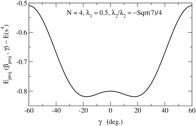
FIG. 2.: The projected energy surface $E_{\rm proj}(\beta,\gamma)$, measured with respect to the energy of the pure configuration, $s^{4}$, along the $\gamma$ direction for $\beta=0.741$. The parameters of the Hamiltonian are taken to be $N=4,\epsilon=1$, $\lambda_{1}=0.5$, and $\lambda_{2}/\lambda_{1}=-\sqrt{7}/4$.

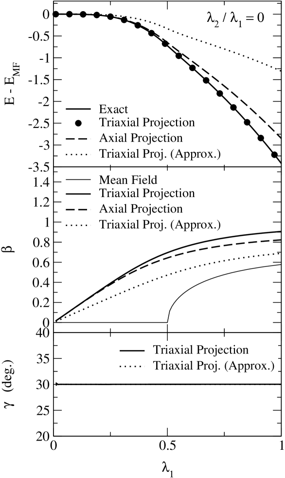
FIG. 3.: Same as fig.1, but for $\lambda_{2}/\lambda_{1}=0$.

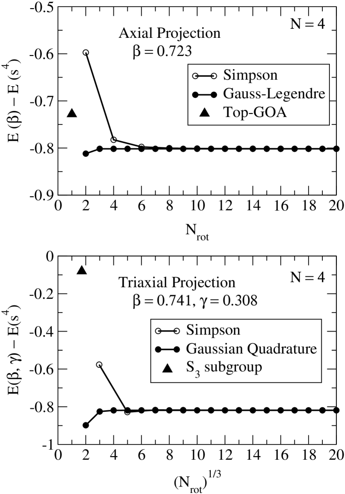
FIG. 4.: Influence of the generator coordinate truncation on the ground state energy. The upper and the lower panels are for the axial and the triaxial projections, respectively. The former plots the energy as a function of the number of rotated wave functions $N_{\rm rot}$, while the latter plots as a function of $(N_{\rm rot})^{1/3}$, for the optimum values of the deformation parameters $\beta$ and $\gamma$ indicated in the insets. The open and the closed circles are the results of the Simpson method and the Gaussian quadrature formula, respectively. The triangles denote the result of the top-GOA approximation (in the upper panel) and that of the approximate projection with the $S_{3}$ subgroup (in the lower panel). The parameters of the Hamiltonian are the same as in fig. 2.

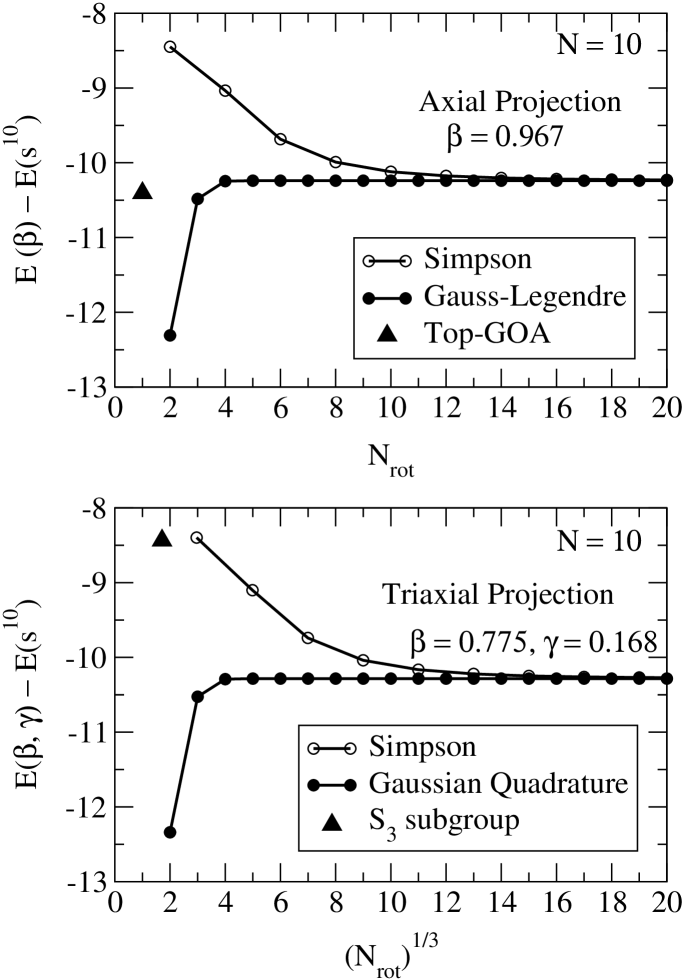
FIG. 5.: Same as fig.4, but for $N=10$.

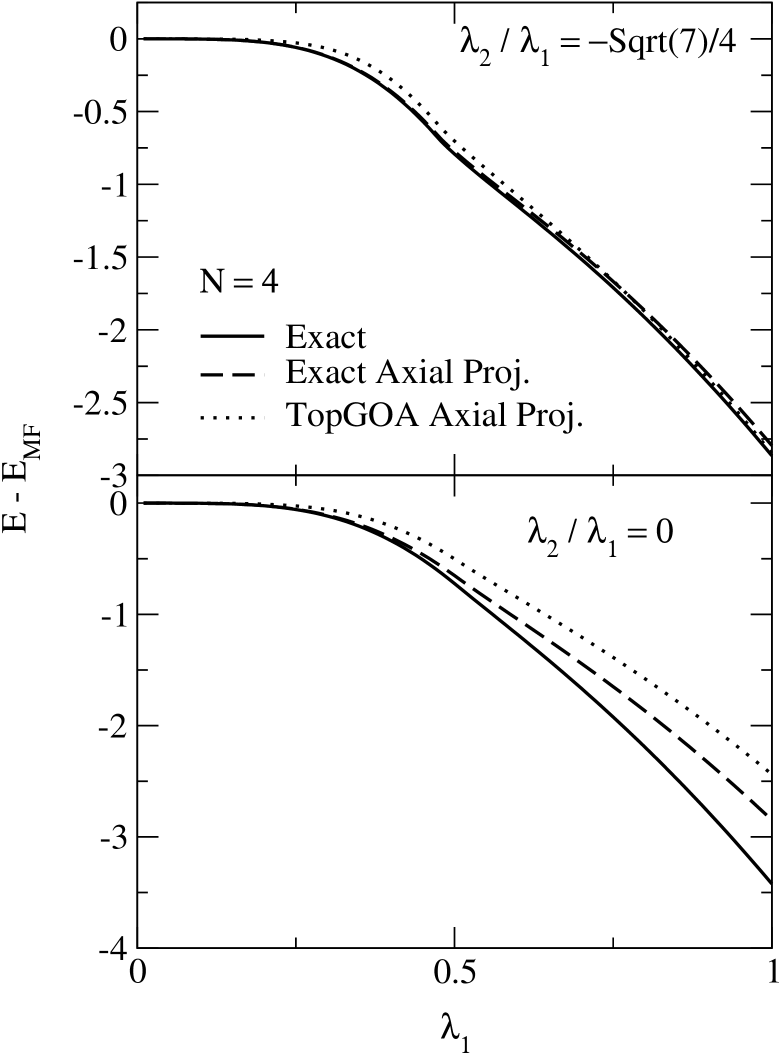
FIG. 6.: The correlation energy obtained in the axially symmetric approximation as a function of $\lambda_{1}$ for $N=4$. The upper and the lower panels are for $\lambda_{2}/\lambda_{1}=-\sqrt{7}/4$ and $\lambda_{2}=0$, respectively. The dashed line is the result of the full axial projection, while the dotted line is obtained in the top-GOA approximation to the axial projection. The exact solution of the Hamiltonian is denoted by the solid line.

REFERENCES

- [1] M. Bender, P.-H. Heenen, and P.-G. Reinhard, Rev. Mod. Phys. 75, 121 (2003).
- [2] K. Hagino and G.F. Bertsch, Phys. Rev. C61, 024307 (2000); Nucl. Phys. A679, 163 (2000).
- [3] K. Hagino, P.-G. Reinhard, and G.F. Bertsch, Phys. Rev. C65, 064320 (2002)
- [4] P.-G. Reinhard, Z. Phys. A285, 93 (1978).
- [5] P. Ring and P. Schuck, The Nuclear Many-Body Problem (Springer-Verlag, New York, 1980).
- [6] F. Iachello and A. Arima, The Interacting Boson Model, (Cambridge University Press, Cambridge, England, 1987).
- [7] J.N. Ginocchio and M.W. Kirson, Phys. Rev. Lett. 44, 1744 (1980); Nucl. Phys. A350, 31 (1980).
- [8] H.J. Lipkin, N. Mechkov, and A.J. Glick, Nucl. Phys. 62, 188 (1965); 62, 199 (1965); 62, 211 (1965).
- [9] P. Bonche, J. Dobaczewski, H. Flocard, and P.-H. Heenen, Nucl. Phys. A530, 149 (1991).
- [10] D. Vautherin, Phys. Rev. C7, 296 (1973).
- [11] Y.K. Gambhir, P. Ring, and A. Thimet, Ann. Phys. (N.Y.) 198, 132 (1990).
- [12] K. Burzynski and J. Dobaczewski, Phys. Rev. C51, 1825 (1995).
- [13] K. Enami, K. Tanabe, and N. Yoshinaga, Phys. Rev. C59, 135 (1999); C63, 044322 (2001).
- [14] P.-G. Reinhard and K. Goeke, Rep. Prog. Phys. 50, 1 (1987).
- [15] J.P. Elliott, Proc. R. Soc. A245, 128 (1958); A245, 562 (1958).
- [16] A. Arima, J. Phys. G25, 581 (1999).
- [17] S. Kuyucak and I. Morrison, Ann. Phys. (N.Y.) 181, 79 (1988); Phys. Rev. C36, 774 (1987).
- [18] M.A. Nagarajan, A.B. Balantekin, and N. Takigawa, Phys. Rev. C34, 894 (1986).
- [19] T. Duguet and P. Bonche, Phys. Rev. C, in press. e-print: nucl-th/0210057.