Many-body approach to proton emission and the role of spectroscopic factors

Abstract

The process of proton emission from nuclei is studied by utilizing the two-potential approach of Gurvitz and Kalbermann in the context of the full many-body problem. A time-dependent approach is used for calculating the decay width. Starting from an initial many-body quasi-stationary state, we employ the Feshbach projection operator approach and reduce the formalism to an effective one-body problem. We show that the decay width can be expressed in terms of a one-body matrix element multiplied by a normalization factor. We demonstrate that the traditional interpretation of this normalization as the square root of a spectroscopic factor is only valid for one particular choice of projection operator. This causes no problem for the calculation of the decay width in a consistent microscopic approach, but it leads to ambiguities in the interpretation of experimental results. In particular, spectroscopic factors extracted from a comparison of the measured decay width with a calculated single-particle width may be affected.

I Introduction

One of the classic problems in quantum mechanics is that of tunneling through a classically forbidden region or, more specifically, the decay of a quasi-stationary state to the continuum. In nuclear physics, this manifests itself in the processes of $\alpha$-decay in heavy nuclei and proton emission by proton drip-line nuclei. Of particular current interest are the lifetimes of proton emitters, especially in the lighter region of the nuclear chart, and the implications of this in nuclear astrophysics.

Over the years, a number of different theoretical approaches have been used to describe the decay process in nuclear physics, either by means of perturbation theory of decaying states or by time reverse study of resonance states via scattering theory Jackson and Rhoades-Brown (1977); Gurvitz et al. ; Mang (1964); Thomas (1954); Arima and Yoshida (1974); Vogt (1996). Some authors solve the time-dependent problem while others use a stationary picture and make use of approximation methods such as the distorted-wave Born approximation or the semi-classical Wentzel-Kramers-Brillouin approach to evaluate the width Åberg et al. (1997). Other more accurate methods, such as R-matrix theory, are sometimes very sensitive to the channel radius giving dramatic variation in the calculated widths Mang (1964); Thomas (1954); Arima and Yoshida (1974); Vogt (1996). The method of Gurvitz and Kalbermann Gurvitz and Kalbermann (1987); Gurvitz (1988); Gurvitz et al. , also known as the two-potential approach (TPA) Jackson and Rhoades-Brown (1977); Åberg et al. (1997), is based on splitting the barrier potential into an interior and an exterior components. The inner potential binds the particle, which can then be described by a bound eigenstate of the relative Hamiltonian, while the outer potential acts as a perturbation that converts it into a quasi-stationary state (a wave packet), which can decay.

An important shortcoming of all the above approaches, however, and in common with the descriptions of so many nuclear processes, is the approximate treatment of the many-body structure effects. In most descriptions of the proton-emission process the initial ($A+1$)-body wave function is written as a product of an $A$-body wave function, describing the daughter nucleus, and the proton’s single-particle wave function. The decay width is then written in the form of a single-particle width multiplied by a spectroscopic factor, which contains the many-body information of the system. This procedure, however, makes various assumptions about the relationship between the many-body problem and the effective one-body problem that have to be tested. In this work we consider the TPA of Gurvitz and Kalbermann and extend it to properly account for the many-body correlations.

The standard reduction from a many-body problem to an effective one-body picture has been revisited in a recent study of radiative proton capture Escher et al. (2001). The work focused on one-body overlap functions and their associated equations of motion. The one-body overlap functions are obtained by integrating the product of the wave functions for an ($A+1$)-body system and its $A$-body subsystem over the coordinates of the latter. While the overlap functions are unambiguously defined, it was demonstrated in Ref. Escher and Jennings (2002) that useful ‘auxiliary’ one-body functions can be defined in several different ways. Naturally, the associated equations of motion differ for the three approaches considered in Ref. Escher and Jennings (2002). In the current work, we derive expressions for the proton decay width using two of the three approaches mentioned. The resulting decay widths have formally the same structure in both approaches, but the overall normalization factors differ. Only one of these normalization factors can be interpreted as the square root of a spectroscopic factor. This has consequences for the interpretation of experimental results and in particular for the determination of spectroscopic factors from decay widths.

We start, in Sec. II, with the time-dependent Schrödinger equation and follow the standard theory of decaying states Goldberger and Watson (1964). This method is briefly compared with the scattering approach to decay problems. In Secs. III and IV we use projection operator techniques and perturbation theory to derive an expression for the decay width in terms of the imaginary part of the pole in the Green’s function matrix element. In Sec. V, we describe the two alternative routes for reducing the many-body problem to an effective one-body problem. We compare the resulting two expressions for the width in Sec. VI. An alternative expression for the decay width is given in Sec. VII which shows more clearly the relation of the width to the spectroscopic factor.

II Proton emission formalism

In this section we begin to recast the formalism of Gurvitz and Kalbermann in a form which is more convenient for our purposes. The approach of Refs. Gurvitz and Kalbermann (1987); Gurvitz (1988) starts with a square-integrable wave function, $|\psi_{0}\rangle$, which corresponds to the quasi-bound nucleus whose decay we are interested in. The initial wave function is close to the resonance state in the nuclear interior but decays rather than oscillates in the exterior region. This wave function cannot be an eigenstate of the full Hamiltonian or it would have a trivial time dependence and no decay would take place. Taking $|\psi_{0}\rangle$ as the wave function at $t=0$, we follow its time evolution using the time-dependent Schrödinger equation:

$$i\hbar\frac{\partial}{\partial t}|\psi(t)\rangle=H|\psi(t)\rangle.$$ (1)

This initial value problem is solved by using the one-sided Fourier transform (sometimes called a Laplace transform). We obtain

$$-i\hbar|\psi_{0}\rangle+E|\tilde{\psi}(E)\rangle = H|\tilde{\psi}(E)\rangle,$$ (2)

where $|\tilde{\psi}(E)\rangle=\int_{0}^{\infty}dt\;e^{i(E+i\epsilon)t/\hbar}|\psi(t)\rangle$ and $\epsilon$ is a positive infinitesimal real number. Solving for $|\tilde{\psi}(E)\rangle$ we have

$$|\tilde{\psi}(E)\rangle = \frac{i\hbar}{E-H+i\epsilon}|\psi_{0}\rangle.$$ (3)

The probability amplitude for the nucleus remaining in the initial state after a time $t$ is given by

$$\langle\psi_{0}|\psi(t)\rangle = \frac{i}{2\pi}\int_{-\infty}^{\infty}dE\;e^{-iEt/\hbar}\langle\psi_{0}|\frac{1}{E-H+i\epsilon}|\psi_{0}\rangle,$$ (4)

which is obtained by taking the matrix element of the previous equation with $\langle\psi_{0}|$ and carrying out the inverse Fourier transform. This is the Fourier transform of one particular matrix element of the many-body Green’s function. In general the Lehmann representation of the latter contains contributions from many poles. However, the overlap $\langle\psi_{0}|\psi(t)\rangle$ takes a simple form if the right-hand side of Eq. (4) is dominated by the contribution of only one pole. In this case the decay rate can be extracted from the imaginary part of the pole location and we obtain a simple exponential function which describes the decay of the initial state. Thus the initial state $|\psi_{0}\rangle$ should be chosen to minimize the contributions from other poles.

The same result can be found by considering the related scattering problem. A quasi-bound state can also be thought of as a resonance in the scattering amplitude. We consider scattering of a proton off the $(A-1)$-body system and we define a t-matrix, $T$, through the equation

$$Ta^{\dagger}(k)|\psi_{A-1}\rangle=V|\psi_{A}\rangle,$$ (5)

where $a^{\dagger}(k)$ is the creation operator for a particle with momentum $k=\sqrt{2mE/\hbar^{2}}$ and $m$ is the reduced mass of the system. By standard techniques it can be shown that

$$T = V+VG_{0}T$$ (6)

$$= V+VGV,$$ (7)

where $G_{0}=1/(E-H_{0}+i\epsilon)$, $G=1/(E-H+i\epsilon)$, and $H_{0}$ describes the free motion of the ejected particle with respect to the final state of the $(A-1)$-body system, i.e., $H_{0}a^{\dagger}(k)|\psi_{A-1}\rangle=Ea^{\dagger}(k)|\psi_{A-1}\rangle$ and $H=H_{0}+V$. We observe that the poles of the t-matrix are given by the poles of $V$ and $G$. Assuming $V$ has no nearby pole we see that the poles of $T$ are just those of the many-body Green’s function. The width of the state is then given by the imaginary part of the pole location as in the previous case.

In principle, the potential $V$ is the sum of the interactions of the $A$-th particle with each of the particles in the $(A-1)$-body system. In nuclear physics this is generally approximated by a nucleon-nucleus optical potential. This approach, however, has the disadvantage of loosing track of the Pauli exchange correlations and other many-body effects. For bound states one of the principal effects is included through the use of the spectroscopic factor. However for scattering states there is, strictly speaking, no spectroscopic factor. Using Eq. (4) as the starting point we can formally take the many-body effects into account while deriving an effective one-body equation.

III Projection operator formalism

The main ingredient of Eq. (4) is the matrix element of the Green’s function, $M=\langle\psi_{0}|\frac{1}{E-H+i\epsilon}|\psi_{0}\rangle$. Its expression can be simplified as done in Ref. Escher and Jennings (2002) by using the projection operator formalism. We define a projection operator $P=|\psi_{0}\rangle\langle\psi_{0}|$ and the complementary operator $Q=1-P$. The equation for the Green’s function can be written as

$$(E-H)\frac{1}{E-H+i\epsilon}=(E-H)G=1.$$ (8)

Acting on the left by $P$ or $Q$ and on the right by $P$ we get the two equations

$$P(E-H)(P+Q)GP = P,$$

$$Q(E-H)(P+Q)GP = 0.$$ (9)

Solving the second equation for $QGP$ and substituting this into the first equation we have

$$\left(E-PHP-PHQ\frac{1}{E-QHQ+i\epsilon}QHP\right)PGP=P.$$ (10)

Taking the matrix element of this equation with $|\psi_{0}\rangle$ and using the explicit form for $P$ we find

$$\left[E-\langle\psi_{0}|\left(H+HQ\frac{1}{E-QHQ+i\epsilon}QH\right)|\psi_{0}\rangle\right]\langle\psi_{0}|G|\psi_{0}\rangle=1.$$ (11)

Since the left-hand side of this equation is a product of two terms, the poles of $\langle\psi_{0}|G|\psi_{0}\rangle$ must coincide with the zeros of the multiplying factor. Thus the poles of the Green’s function are given by

$$E=\langle\psi_{0}|\left(H+HQ\frac{1}{E-QHQ+i\epsilon}QH\right)|\psi_{0}\rangle\;,$$ (12)

or, if we use a spectral representation of $\frac{1}{E-QHQ+i\epsilon}$, by

$$E = \langle\psi_{0}|H|\psi_{0}\rangle+\int_{-\infty}^{\infty}dE^{\prime}\;\frac{|\langle\psi_{0}|HQ|\zeta_{E^{\prime}}\rangle|^{2}}{E-E^{\prime}+i\epsilon},$$ (13)

where $|\zeta_{E^{\prime}}\rangle$ is the solution of the equation

$$E|\zeta_{E}\rangle=QHQ|\zeta_{E}\rangle,$$ (14)

normalized according to $\langle\zeta_{E}^{\prime}|\zeta_{E}\rangle=\delta(E^{\prime}-E)$. Note that $|\psi_{0}\rangle$ is also an eigenstate of $QHQ$, but with energy $E=0$. This state is excluded from the sum (integral) in Eq. (13) by the projection operator. In fact the only role of $Q$ in this equation is to exclude the discrete state $|\psi_{0}\rangle$. The residue, $R$, of the pole of $\langle\psi_{0}|G|\psi_{0}\rangle$ is given by

$$R=\left[1-\frac{d}{dE}\langle\psi_{0}|HQ\frac{1}{E-QHQ+i\epsilon}QH|\psi_{0}\rangle\right]^{-1}.$$ (15)

This follows from a Taylor series expansion of Eq. (11) in $E$. For the present problem $R$ is close to one since we will choose $|\psi_{0}\rangle$ to be an eigenvalue of $H$ inside the nucleus and different from an eigenstate only in a region where the wave function is exponentially damped. Where $|\psi_{0}\rangle$ is an eigenstate $\langle\psi_{0}|HQ$ is zero so the contribution from the second term will be exponentially small.

More insight into Eq. (12) can be obtained by an alternative derivation. Consider the equation $E=\langle\psi_{0}|H|\psi_{E}\rangle/\langle\psi_{0}|\psi_{E}\rangle$ where $|\psi_{E}\rangle$ is an eigenstate of the full Hamiltonian, $H$. The wave function can be written as $|\psi_{E}\rangle=(P+Q)|\psi_{E}\rangle$. Following the standard Feshbach projection operator technique we can write $Q|\psi_{E}\rangle=Q\frac{1}{E-QHQ+i\epsilon}QHP|\psi_{E}\rangle$. Using the explicit form of the projection operator $P=|\psi_{0}\rangle\langle\psi_{0}|$ yields Eq. (12) immediately.

IV Perturbative approximation

In general, Eq. (12) is highly non-linear and has many solutions. Every solution of this equation will give a pole of the Green’s function, however, not every pole of the Green’s function will necessarily be found by using this equation. For example, if $|\psi_{0}\rangle$ has a definite angular momentum only poles with that angular momentum can be found with that particular choice of $|\psi_{0}\rangle$.

For the problem at hand, namely proton emission, we are not interested in the complete complexity of the Green’s function. To obtain the decay width, only the imaginary part of the pole location of the nearby pole is relevant. We define an Hermitian Hamiltonian $H_{0}$ such that $H_{0}|\psi_{0}\rangle=E_{0}|\psi_{0}\rangle$ with $H=H_{0}+\delta H$. Expanding the right hand side of Eq. (12) about $E_{0}$ and neglecting terms of order $(E-E_{0})^{2}$ we obtain

$$E-E_{0} \approx \langle\psi_{0}|\delta H|\psi_{0}\rangle+\langle\psi_{0}|HQ\frac{1}{E_{0}-QHQ+i\epsilon}QH|\psi_{0}\rangle$$ (16)

$$+(E-E_{0})\left[\frac{d}{dE}\langle\psi_{0}|HQ\frac{1}{E-QHQ+i\epsilon}QH|\psi_{0}\rangle\right]_{E=E_{0}}$$

$$\approx R\left(\langle\psi_{0}|\delta H|\psi_{0}\rangle+\langle\psi_{0}|HQ\frac{1}{E_{0}-QHQ+i\epsilon}QH|\psi_{0}\rangle\right),$$ (17)

where the last line has been obtained by solving for $(E-E_{0})$ in the first equation. This expression for the energy, Eq. (17), contains a factor of $R$, the residue of pole of $\langle\psi_{0}|G|\psi_{0}\rangle$. Note that $\langle\psi_{0}|HQ=\langle\psi_{0}|\delta HQ$ implies that $R-1$ is of the order of $\delta H^{2}$. Since it multiplies a factor of order $\delta H$, it will introduce terms of order higher than $(E-E_{0})^{2}\approx\delta H^{2}$ and therefore it can be neglected. In the following, we thus take $R=1$.

Let us emphasize that $E_{0}$ is real since it is an the eigenvalue of the Hermitian operator $H_{0}$. The pole location, on the other hand, occurs at a complex energy. If the width of the state is large, for any reason not just proton emission, then $E\approx E_{0}$ does not hold (since $E_{0}$ is real and the pole location has a large imaginary part) and the approximation fails. However, when the width is narrow then it will be possible to chose $|\psi_{0}\rangle$ or equivalently $H_{0}$ such that perturbation theory is applicable.

The equation for the energy is now linear in $E$ and has the form typical of perturbation theory. The explicit connection with perturbation theory can be made when the unperturbed Hamiltonian is taken to be $H_{00}=H_{0}+Q\delta HQ$, and not $H_{0}$ as one might have expected. This definition is not only necessary in order to cast Eq. (13) into the form of a perturbation expansion but at the same time eliminates the problem of non-compactness Gurvitz and Kalbermann (1987); Gurvitz (1988). The non-compactness arises since $H_{0}$ is chosen in such a manner that it does not go to zero at infinity. However both $H$ and $H_{00}$ go to zero at infinity.

The states $|\zeta_{E}\rangle$ occurring in the integral in Eq. (13) are eigenstates of $H_{00}$, as is $|\psi_{0}\rangle$. In contrast to Eq. (14) the state $|\psi_{0}\rangle$ now occurs with energy $E_{0}$ rather than $0$. We can also rewrite $\langle\psi_{0}|HQ|\zeta_{E^{\prime}}\rangle$ as $\langle\psi_{0}|(H-H_{0})Q|\zeta_{E^{\prime}}\rangle$ or $\langle\psi_{0}|(H-H_{00})Q|\zeta_{E^{\prime}}\rangle$ since $\langle\psi_{0}|$ is an eigenstate of both $H_{0}$ and $H_{00}$ or, equivalently, since $Q$ commutes with both $H_{0}$ and $H_{00}$. Using the previously defined $\delta H=H-H_{0}$, Eq. (13) can be rewritten as

$$E \approx E_{0}+\langle\psi_{0}|\delta H|\psi_{0}\rangle+\int_{-\infty}^{\infty}dE^{\prime}\;\frac{|\langle\psi_{0}|\delta HQ|\zeta_{E^{\prime}}\rangle|^{2}}{E_{0}-E^{\prime}+i\epsilon}$$ (18)

$$\approx E_{0}+\langle\psi_{0}|\delta H^{\prime}|\psi_{0}\rangle+\int_{-\infty}^{\infty}dE^{\prime}\;\frac{|\langle\psi_{0}|\delta H^{\prime}Q|\zeta_{E^{\prime}}\rangle|^{2}}{E_{0}-E^{\prime}+i\epsilon},$$ (19)

where

$$\delta H^{\prime}=H-H_{00}=P\delta H+\delta HP-P\delta HP.$$ (20)

Equation (18) for $E$ is not in the form of perturbation theory since $|\zeta_{E}\rangle$ is an eigenfunction of $H_{00}$ and not $H_{0}$. However, Eq. (19) is. The only approximation made in deriving Eqs. (18) and (19) was the replacement of $E$ in the denominator on the right hand side by $E_{0}$, i.e., we assumed that perturbation theory is valid.

We emphasize that neither $|\psi_{0}\rangle$ nor $|\zeta_{E}\rangle$ is an eigenstate of the full Hamiltonian $H$ and our derivation depends crucially on this point. Instead, $|\psi_{0}\rangle$ is an eigenstate of $H_{0}$ and $H_{00}$ while $|\zeta_{E}\rangle$ is an eigenstate of $QHQ$ and $H_{00}$. The fact that both wave functions are eigenstates of $H_{00}$ allows us to interpret the right-hand side of Eq. (19) as the first few terms of a perturbative expansion.

V Choice of $H_{0}$

The proper choice of $H_{0}$ was discussed in a very convincing and direct way by Gurvitz and Kalbermann Gurvitz and Kalbermann (1987); Gurvitz (1988) for the problem of a single particle in a local potential well. The reader is referred to those papers for specific details. The basic idea is to take an $H_{0}$ such that at infinity the potential goes to a finite value, larger than $E_{0}$, rather than to zero. This causes the state under consideration to be bound, but if the decay width is small this new state should be very close to the scattering state. We now generalize this concept to the case of $A$ interacting particles.

We consider the case where there is one open channel. Asymptotically the wave function describes a free proton and the bound $(A-1)$-body system. Thus we take

$$\delta H=-\int d\mathbf{r}\;a^{\dagger}(\mathbf{r})|\Phi_{A-1}\rangle V(\mathbf{r})\langle\Phi_{A-1}|a(\mathbf{r}),$$ (21)

where $|\Phi_{A-1}\rangle$ is the ground state of the $(A-1)$-body system, $\mathbf{r}$ is the relative coordinate of the proton and the $(A-1)$-body system. The integral covers the whole space. If $V(\mathbf{r})$ is taken to be greater than $E_{0}$ outside the range of the nuclear potential, $r_{0}$, it will prevent the initial state $|\psi_{0}\rangle$ from decaying. At the same time, we want the perturbing potential $V(\mathbf{r})$ to be zero inside the nucleus so that it does not modify the wave function in the interior. With this ansatz expression (18) for $E$ becomes

$$E \approx E_{0}-\int d\mathbf{r}\;\phi^{*}_{0}(\mathbf{r})V(\mathbf{r})\phi_{0}(\mathbf{r})+\int_{-\infty}^{\infty}dE^{\prime}\;\frac{|\int d\mathbf{r}\;\phi^{*}_{0}(\mathbf{r})V(\mathbf{r})\phi_{E^{\prime}}(\mathbf{r})|^{2}}{E_{0}-E^{\prime}+i\epsilon},$$ (22)

where $\phi_{0}(\mathbf{r})=\langle\Phi_{A-1}|a(\mathbf{r})|\psi_{0}\rangle$ is a spectroscopic amplitude (i.e. a one-body overlap function involving bound many-body states) and $\phi_{E^{\prime}}(\mathbf{r})=\langle\Phi_{A-1}|a(\mathbf{r})|\zeta_{E^{\prime}}\rangle$ is an optical model wave function (cf. the discussion in Refs. Escher et al. (2001); Escher and Jennings (2002)). The projection operator $Q$ does not have to be included explicitly since the integral does not include the discrete state $\phi_{0}(\mathbf{r})$.

A miracle has occurred here. Due to the choice of $\delta H$, which is physically motivated, the expression has reduced to an effective one-body problem. All the many-body aspects of the problem are contained in the one-body overlap functions, $\phi_{0}(\mathbf{r})$ and $\phi_{E^{\prime}}(\mathbf{r})$. We stress that the only approximation made so far is that second order perturbation theory was used to justify replacing $E$ with $E_{0}$ in Eq. (13). For states with narrow widths this should be acceptable. We have not assumed that $|\psi_{0}\rangle$ is a product state or made any other assumptions regarding its structure.

Equation (14) for $|\zeta_{E}\rangle$ can be written as $E|\zeta_{E}\rangle=H_{00}|\zeta_{E}\rangle$. In the neighborhood of $E=E_{0}$ the Hamiltonian in this equation for $|\zeta_{E^{\prime}}\rangle$ can be approximated as

$$\delta H^{\prime} \approx -\int d\mathbf{r}\;a^{\dagger}(\mathbf{r})|\Phi_{A-1}\rangle V_{00}(\mathbf{r})\langle\Phi_{A-1}|a(\mathbf{r}).$$ (23)

For an appropriately chosen $V_{00}(\mathbf{r})$, the approximation made here is the same as that of Eq. (2.15) in Ref. Gurvitz and Kalbermann (1987). The basic argument given there proceeds as follows: the eigenfunction of $H$ at resonance will be large when the $A$th particle is in the nuclear interior. However the state $|\zeta_{E^{\prime}}\rangle$ will be small due to the projection operators in $QHQ$. It will look like the real state in exterior region but be suppressed in the interior. The form of $V_{00}(\mathbf{r})$ will ensure this if we take it to be $0$ in the exterior region and repulsive (greater than $E_{0}$) in the interior region (see Fig. 3 in Ref. Gurvitz and Kalbermann (1987)). This is the opposite of what we did for $V(\mathbf{r})$ which was large in the exterior and $0$ in the interior.

Despite its nice form, Eq. (22) is not useful until we specify how to calculate the functions $\phi_{0}(\mathbf{r})$ and $\phi_{E^{\prime}}(\mathbf{r})$. Following Ref. Escher and Jennings (2002) we set up one-body equations for these functions using the Feshbach projection operator technique. We start with the exact scattering state $|\Phi_{A}\rangle$ and write the equation-of-motion for the corresponding one-body overlap function (which in this case is the Feshbach optical model wave function) and see how it is modified when the perturbing Hamiltonian $\delta H$ is added. The one-body overlap function for the exact scattering state is given by Feshbach (1958, 1962); Block and Feshbach (1963); Escher and Jennings (2002)

$$E\phi(\mathbf{r}) = \int d\mathbf{r}^{\prime}d\mathbf{r}^{\prime\prime}\langle\Phi_{A-1}|a(\mathbf{r})\left(H+HQ_{F}\frac{1}{E-Q_{F}HQ_{F}}Q_{F}H\right)a^{\dagger}(\mathbf{r}^{\prime\prime})|\Phi_{A-1}\rangle$$ (24)

$$\hskip 56.9055pt{\cal N}(\mathbf{r}^{\prime\prime},\mathbf{r}^{\prime})^{-1}\phi(\mathbf{r}^{\prime})$$

$$= \int d\mathbf{r}^{\prime}{\cal H}(\mathbf{r},\mathbf{r}^{\prime})\phi(\mathbf{r}^{\prime}),$$ (25)

where $P_{F}=\int d\mathbf{r}d\mathbf{r}^{\prime}\;a^{\dagger}(\mathbf{r})|\Phi_{A-1}\rangle{\cal N}(\mathbf{r},\mathbf{r}^{\prime})^{-1}\langle\Phi_{A-1}|a(\mathbf{r}^{\prime})$, $Q_{F}=1-P_{F}$ and the norm operator is ${\cal N}(\mathbf{r},\mathbf{r}^{\prime})=\langle\Phi_{A-1}|a(\mathbf{r})a^{\dagger}(\mathbf{r}^{\prime})|\Phi_{A-1}\rangle$. Since $\delta HQ_{F}=Q_{F}\delta H=0$, it follows that $\phi_{0}(\mathbf{r})$ satisfies the equation

$$E\phi_{0}(\mathbf{r})=\int d\mathbf{r}^{\prime}\left[{\cal H}(\mathbf{r},\mathbf{r}^{\prime})+{\cal N}(\mathbf{r},\mathbf{r}^{\prime})V(\mathbf{r}^{\prime})\right]\phi_{0}(\mathbf{r}^{\prime}).$$ (26)

Note the explicit asymmetry of this Hamiltonian. Even in the absence of inelastic processes it is not Hermitian. An analogous potential in alpha emission has been strongly criticized Varga and Lovas (1991); Lovas et al. (1998) in the study of alpha emission. Two methods of addressing the problem were discussed in Ref. Escher and Jennings (2002). The first is to define a new amplitude $\bar{\phi}(\mathbf{r})=\int d\mathbf{r}^{\prime}\;{\cal N}(\mathbf{r},\mathbf{r}^{\prime})^{-1/2}\phi(\mathbf{r}^{\prime})$ and take

$$\delta H=-\int d\mathbf{r}d\mathbf{r}^{\prime}d\mathbf{r}^{\prime\prime}a^{\dagger}(\mathbf{r})|\Phi_{A-1}\rangle{\cal N}(\mathbf{r},\mathbf{r}^{\prime})^{-1/2}\bar{V}(\mathbf{r}^{\prime}){\cal N}(\mathbf{r}^{\prime},\mathbf{r}^{\prime\prime})^{-1/2}\langle\Phi_{A-1}|a(\mathbf{r}^{\prime\prime}).$$ (27)

The equation for $\bar{\phi}(\mathbf{r})$ is then

$$E\bar{\phi}_{0}(\mathbf{r})=\int d\mathbf{r}^{\prime}\left[\bar{\cal H}(\mathbf{r},\mathbf{r}^{\prime})+\delta(\mathbf{r},\mathbf{r}^{\prime})\bar{V}(\mathbf{r}^{\prime})\right]\bar{\phi}_{0}(\mathbf{r}^{\prime}),$$ (28)

where $\bar{\cal H}(\mathbf{r},\mathbf{r}^{\prime})$ is given in Ref. Escher and Jennings (2002) as

$$\bar{\cal H}(\mathbf{r},\mathbf{r}^{\prime})=\int d\mathbf{r}^{\prime\prime}d\mathbf{r}^{\prime\prime\prime}{\cal N}(\mathbf{r},\mathbf{r}^{\prime\prime})^{-1/2}{\cal H}(\mathbf{r}^{\prime\prime},\mathbf{r}^{\prime\prime\prime}){\cal N}(\mathbf{r}^{\prime\prime\prime},\mathbf{r}^{\prime})^{1/2}.$$ (29)

A similar development holds for $\phi_{E}(\mathbf{r})$ and we obtain the corresponding equation

$$E\bar{\phi}_{E}(\mathbf{r})=\int d\mathbf{r}^{\prime}\left[\bar{\cal H}(\mathbf{r},\mathbf{r}^{\prime})+\delta(\mathbf{r},\mathbf{r}^{\prime})\bar{V}_{00}(\mathbf{r}^{\prime})\right]\bar{\phi}_{E}(\mathbf{r}^{\prime}).$$ (30)

The equations we find for $\bar{\phi}_{0}(\mathbf{r})$ and $\bar{\phi}_{E}(\mathbf{r})$ are quite remarkable. As previously noted, we have reduced the many-body problem to an effective one-body equation in which all many-body effects are contained in $\bar{\cal H}(\mathbf{r},\mathbf{r}^{\prime})$. The perturbing potential is taken to be local in both cases. This is not really an additional approximation since the justifications given previously still hold.

Another way of getting a symmetric form for the additional potential is by using a projection operator given in Ref. Escher and Jennings (2002)

$$P_{F}=\int d\mathbf{r}\;[a(\mathbf{r})+a^{\dagger}(\mathbf{r})]|\Phi_{A-1}\rangle\langle\Phi_{A-1}|[a(\mathbf{r})+a^{\dagger}(\mathbf{r})]\;,$$ (31)

for which Eq. (26) reduces to the Dyson equation of many-body theory. For time reversal invariant states the associated norm operator reduces to the unity operator. Repeating the derivation with this new projection operator we obtain

$$E\phi_{0}(\mathbf{r}) = \int d\mathbf{r}^{\prime}\left[{\cal H_{M}}(\mathbf{r},\mathbf{r}^{\prime})+\delta(\mathbf{r},\mathbf{r}^{\prime})V(\mathbf{r}^{\prime})\right]\phi_{0}(\mathbf{r}^{\prime}),$$ (32)

$$E\phi_{E}(\mathbf{r}) = \int d\mathbf{r}^{\prime}\left[{\cal H_{M}}(\mathbf{r},\mathbf{r}^{\prime})+\delta(\mathbf{r},\mathbf{r}^{\prime})V_{00}(\mathbf{r}^{\prime})\right]\phi_{E}(\mathbf{r}^{\prime}),$$ (33)

where ${\cal H_{M}}(\mathbf{r},\mathbf{r}^{\prime})$ is the mass operator that occurs in the particle-hole Green’s function Escher and Jennings (2002). In general there is no simple relation between ${\cal H_{M}}(\mathbf{r},\mathbf{r}^{\prime})$ and $\bar{\cal H}(\mathbf{r},\mathbf{r}^{\prime})$. The equations for $\phi(\mathbf{r})$ and $\bar{\phi}(\mathbf{r})$ are now formally the same. At this point we would expect the widths calculated with these functions to be numerically similar. The only difference in the two treatments is the form of $V(\mathbf{r})$ and $V_{00}(\mathbf{r})$. When the argument leading to the justification of perturbation theory is correct we expect both approaches to work equally well.

The argument for Eq. (23) can be restated using the one-body functions defined above. The resonant state, that is the solution of the exact Schrödinger-like equation $E_{0}\phi_{0}^{\rm true}(\mathbf{r})=\int d\mathbf{r}^{\prime}\;{\cal H}(\mathbf{r},\mathbf{r}^{\prime})\phi_{0}^{\rm true}(\mathbf{r}^{\prime})$, grows exponentially as we go into the classical forbidden region under the Coulomb barrier from the outside and the wave function is exponentially large in the interior. On the other hand, $\phi_{E}(\mathbf{r})$ coming from $|\zeta_{E}\rangle$, the solution of the many body-state defined with the Hamiltonian $QHQ$, is exponentially suppressed due to the orthogonality of $|\psi_{0}\rangle$ and $|\zeta_{E}\rangle$. If the suppression is large (i.e. the state under consideration is narrow) the precise form of $|\zeta_{E}\rangle$ in the interior is not important as it is essentially zero. The approximate form of $H_{00}$ is chosen so the approximate $|\zeta_{E}\rangle$ is also zero in the interior. As we will see later we do not need $|\zeta_{E}\rangle$ in the interior but only outside at some radius, $r_{0}$.

VI Two expressions for the width

The decay width is given in terms of the imaginary part of the pole location in Eq. (22). We find

$$\Gamma_{0} \approx 2\pi\left|\int d\mathbf{r}\;\phi^{*}_{0}(\mathbf{r})V(\mathbf{r})\phi_{E_{0}}(\mathbf{r})\right|^{2}$$ (34)

or

$$\Gamma_{0} \approx 2\pi\left|\int d\mathbf{r}\;\bar{\phi}^{*}_{0}(\mathbf{r})\bar{V}(\mathbf{r})\bar{\phi}_{E_{0}}(\mathbf{r})\right|^{2},$$ (35)

depending on whether we use the bar-ed amplitudes or the standard overlap functions. As discussed below, we expect the approximations leading to the two equations to be valid simultaneously, so that the resulting two expressions for the width will agree. We stress again that the reduction to an effective one-body problem is not an approximation but emerges rather naturally from the formalism. In a pure one-body problem $\phi_{0}(\mathbf{r})$ and $\bar{\phi}_{0}(\mathbf{r})$ would be normalized to unity whereas here they are normalized to the factors $\sqrt{S_{0}}$ and $\sqrt{\bar{S}_{0}}$, respectively. The normalization factors contain the many-body aspects of the problem. For the standard overlap function $\phi_{0}(\mathbf{r})$, this normalization is the well-known spectroscopic factor (see also Ref. Escher and Jennings (2002)). It is useful to define normalized one-body functions $\hat{\phi}_{0}(\mathbf{r})$ and $\hat{\bar{\phi}}_{0}(\mathbf{r})$ via $\phi_{0}(\mathbf{r})=\sqrt{S_{0}}\hat{\phi}_{0}(\mathbf{r})$ and $\bar{\phi}_{0}(\mathbf{r})=\sqrt{\bar{S}_{0}}\hat{\bar{\phi}}_{0}(\mathbf{r})$ (i.e. $\int d\mathbf{r}|\hat{\phi}_{0}(\mathbf{r})|^{2}=\int d\mathbf{r}|\hat{\bar{\phi}}(\mathbf{r})_{0}|^{2}=1$). The wave-functions $\phi_{E_{0}}(\mathbf{r})$ and $\bar{\phi}_{E_{0}}(\mathbf{r})$ describe scattering states and are normalized asymptotically at large $r$. If we assume the one-body Hamiltonians ${\cal H}$ and ${\bar{\cal H}}$ to be local (more will be said about this later) we can take over verbatim the development given in Refs. Gurvitz and Kalbermann (1987); Gurvitz (1988); Gurvitz et al. . The only difference between the treatment presented there and the approach shown here is the presence of the factors $S_{0}$ (for the standard overlap functions) and $\bar{S}_{0}$ (for the bar-ed function). To make the dependence on these normalization factors explicit we rewrite the last equations as

$$\Gamma_{0} \approx 2\pi S_{0}\left|\int d\mathbf{r}\;\hat{\phi}^{*}_{0}(\mathbf{r})V(\mathbf{r})\phi_{E_{0}}(\mathbf{r})\right|^{2}$$ (36)

and

$$\Gamma_{0} \approx 2\pi\bar{S}_{0}\left|\int d\mathbf{r}\;\hat{\bar{\phi}}^{*}_{0}(\mathbf{r})\bar{V}(\mathbf{r})\bar{\phi}_{E_{0}}(\mathbf{r})\right|^{2}.$$ (37)

To further understand the results we peruse one particular line of development. As previously noted, we take $V(\mathbf{r})$ to be zero inside the nucleus, $V(\mathbf{r})=0$ for $r\leq r_{0}$. For $r\geq r_{0}$, we have $\int d\mathbf{r}^{\prime}{\cal H_{M}}(\mathbf{r},\mathbf{r}^{\prime})\phi_{E}(\mathbf{r}^{\prime})=E\phi_{E}(\mathbf{r})$ since $V_{00}(\mathbf{r})$ vanishes for large $r$. For definiteness we follow Refs. Gurvitz and Kalbermann (1987); Gurvitz (1988) and take $r_{0}$ to the maximum of the potential. For the example of fluorine discussed below, this corresponds to about 5 fm. Thus we write the integral in Eq. (34) as

$$I = \int d\mathbf{r}\;\theta(r-r_{0})\phi^{*}_{0}(\mathbf{r})V(\mathbf{r})\phi_{E_{0}}(\mathbf{r})$$ (38)

$$= \int d\mathbf{r}d\mathbf{r}^{\prime}\;\theta(r-r_{0})\phi^{*}_{0}(\mathbf{r})\left\{{\cal H_{M}}(\mathbf{r},\mathbf{r}^{\prime})+[-E_{0}+V(\mathbf{r})]\delta(\mathbf{r},\mathbf{r}^{\prime})\right\}\phi_{E_{0}}(\mathbf{r}),$$ (39)

with a similar equation holding for the bar-ed quantity. Naively one might expect this to vanish and indeed it would if the step function $\theta$ were not there. In the following we shall consider the case in which the non-locality in ${\cal H_{M}}(\mathbf{r},\mathbf{r}^{\prime})$ is small enough to be properly described by a local potential and an effective mass $m_{k}(\mathbf{r})$. In this case one has Ma and Wambach (1983)

$${\cal H_{M}}(\mathbf{r},\mathbf{r}^{\prime})=\left[\nabla\frac{-\hbar^{2}}{2m_{k}(\mathbf{r})}\nabla+V_{\cal M}(\mathbf{r})\right]\delta(\mathbf{r},\mathbf{r}^{\prime})\;.$$ (40)

In this equation ${\cal H_{M}}$ is correctly evaluated at the energy $E_{0}$ of the scattered state, therefore $m_{k}(\mathbf{r})$ accounts for the sole spatial non-locality and differs from the usual definition of effective mass $m^{*}(\mathbf{r})$ Negele and Yazaki (1981); Jaminon and Mahaux (1989). When Eq. (40) holds, the integral, Eq. (39), can be simplified through integration by parts and, for spherically symmetric potentials $V(r)$, $V_{\cal M}(r)$ and effective mass $m_{k}(r)$, one obtains

$$I = \frac{\hbar^{2}}{2m_{k}(r_{0})}\left[\phi_{\mathrm{r}0}^{*}(r_{0})\phi_{\mathrm{r}E_{0}}^{\prime}(r_{0})-\phi_{\mathrm{r}E_{0}}(r_{0})\phi^{\prime*}_{\mathrm{r}0}(r_{0})\right]$$ (41)

$$= \frac{\hbar^{2}}{2\bar{m}_{k}(r_{0})}\left[\bar{\phi}_{\mathrm{r}0}^{*}(r_{0})\bar{\phi}_{\mathrm{r}E_{0}}^{\prime}(r_{0})-\bar{\phi}_{\mathrm{r}E_{0}}(r_{0})\bar{\phi}^{\prime*}_{\mathrm{r}0}(r_{0})\right],$$ (42)

where the wave functions are assumed to factorize as $\phi(\mathbf{r})=\frac{\phi_{\mathrm{r}}(r)}{r}Y_{\ell}^{m}(\theta,\varphi)$ and $Y_{\ell}^{m}(\theta,\varphi)$ are spherical harmonic functions of the angular variables $\theta,\varphi$. The prime denotes the derivation with respect to the radial coordinate $r$.

In deriving these last two equations we made an additional approximation, namely that the potentials are local in the vicinity of $r_{0}$ [or at least the non-locality is restricted to an effective mass $m_{k}(r)$]. The two equations will be simultaneously valid only if the norm operator is local, i.e.  ${\cal N}(\mathbf{r},\mathbf{r}^{\prime})={\cal N}(\mathbf{r})\delta(\mathbf{r}-\mathbf{r}^{\prime})$, in the vicinity of $r_{0}$. In this case $\bar{m}_{k}(r_{0})/m_{k}(r_{0})={\cal N}(r_{0})$ and the two equations are identical. Since $r_{0}$ is in the tail of the density distribution, one expects the norm operator to be unity in its vicinity, which means that the two expressions for the width should give the same result for realistic models. This is verified numerically in Fig. 1, where the function $\phi_{\mathrm{r}}(r)$ (solid lines) and $\bar{\phi}_{\mathrm{r}}(r)$ (dashed lines) are displayed for the $3/2^{-}$ and $3/2^{+}$ decaying states of ¹⁷F at respective excitation energies of 4.64 and 5.00 MeV (the proton threshold is at 0.60 MeV). The functions are calculated with the self-consistent Green’s function method of Refs. Barbieri and Dickhoff (2001, 2002); Barbieri (2002). The $3/2^{+}$ state is well explained by the nuclear mean field approach and provides a typical example of a strong state, for which $S_{0}\approx\bar{S}_{0}$. The $3/2^{-}$ state, on the other hand, is a typical example of a weak state for which Ref. Barbieri (2002) gives $S_{0}\approx 0.04$ and $\bar{S}_{0}\approx 0.14$. It is worth to emphasize the difference between these two cases. For strong states the quenching of the spectroscopic factor is due both to short-range correlations and to the coupling to other excitations of the system Barbieri and Dickhoff (2002). Nevertheless they maintain a strong single-particle structure and the orbital occupancy is of the order of unity. Weak states, instead, have a more complicated structure and can be seen as collective excitations on their own rather than having a single-particle character. As a consequence the one-body spectroscopic factor can be one order of magnitude smaller or less. In this case the functions $\phi(\mathbf{r})$ and $\bar{\phi}(\mathbf{r})$ sample the one-body substructure in a different way, whence the difference in their normalizations with $\bar{S}_{0}$ larger than $S_{0}$ Escher and Jennings (2002). For ¹⁶O + p, the nuclear interaction becomes negligible beyond 5 fm typically and Fig. 1 shows that $\phi(\mathbf{r})$ and $\bar{\phi}(\mathbf{r})$ are equal beyond this radius, which means that the norm operator is unity. In principle, there is no problem calculating the width from a microscopic model: one may define two different functions $\phi(\mathbf{r})$ and $\bar{\phi}(\mathbf{r})$, which have two different normalization factors $\sqrt{S}$ and $\sqrt{\bar{S}}$, respectively, but the estimate for the width will be the same with both of them. In fact, a similar formula would be valid for any amplitude of the form $\phi^{\nu}(\mathbf{r})=\int dr^{\prime}\;{\cal N}(\mathbf{r},\mathbf{r}^{\prime})^{\nu}\phi(\mathbf{r}^{\prime})$ for arbitrary $\nu$, since ${\cal N}(\mathbf{r},\mathbf{r}^{\prime})$ is unity around $r_{0}$.

Let us emphasize that for the actual calculation of the width by the above formulas, a microscopic model based on the harmonic oscillator basis, as in Refs. Barbieri and Dickhoff (2002); Barbieri (2002) may not be the best choice since the wave function is not expected to be very precise in the vicinity of $r_{0}$. This is demonstrated in Fig. 1, where the $3/2^{+}$ resonant wave function of the phenomenological mean field Woods-Saxon potential of Ref. Sparenberg et al. (2000) is shown for comparison. The agreement with the microscopic wave function is good in the interior but deteriorates above 4 fm (where the approximation of the potential by a harmonic oscillator breaks down, see Fig. 2). The difference between both models is particularly large in this case since the $3/2^{+}$ state is wide ($\Gamma_{0}=1.5$ MeV); for narrow states, the harmonic oscillator approximation could be sufficient, a possibility which will be explored elsewhere. Let us finally stress that the phenomenological mean field potential of Ref. Sparenberg et al. (2000) does not reproduce the $3/2-$ state because its structure is not well approximated by an ¹⁶O core plus a proton.

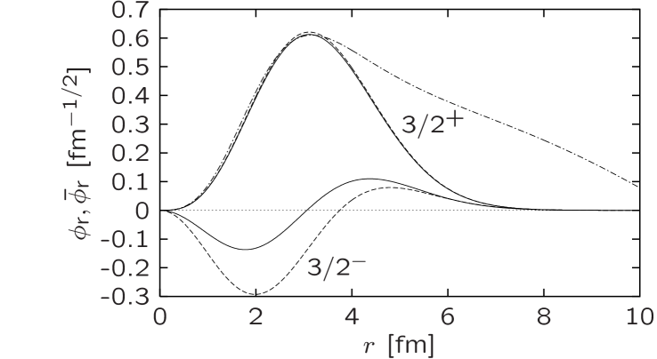
Figure 1: Radial part of the one-body overlap functions $\phi$ (solid lines) and of the auxiliary functions $\bar{\phi}$ (dashed lines) for the lowest $3/2^{-}$ and $3/2^{+}$ states of ¹⁷F, calculated via the self-consistent Green’s function method. For the $3/2^{+}$ state, both functions are nearly identical, and a phenomenological wave function, with a normalization chosen to be close to that of the microscopic wave functions, is shown for comparison (dash-dotted line).

Equations (36) and (37) indicate that there may be a serious problem in extracting spectroscopic factors from measured decay widths. The standard method for determining a spectroscopic factor involves dividing an experimental width by a single-particle width calculated with a phenomenological model. However, it is not clear a priori whether the phenomenological wave functions are good approximations to $\hat{\phi}_{0}(\mathbf{r})$ and $\phi_{E}(\mathbf{r})$, or to $\hat{\bar{\phi}}_{0}(\mathbf{r})$ and $\bar{\phi}_{E}(\mathbf{r})$; hence, it is not obvious whether dividing the experimental width by the result of a single-particle calculation provides the spectroscopic factor $S_{0}$ or the normalization $\bar{S}_{0}$ of the auxiliary function $\bar{\phi}(\mathbf{r})$ (or the norm of yet another one-body function). Normally, one assumes in proton emission studies that $\hat{\phi}_{0}(\mathbf{r})$ and $\phi_{E}(\mathbf{r})$ can be equated with the wave functions obtained from phenomenological potentials (see for example Ref. Åberg et al. (1997)). On the other hand, in the context of some alpha emission studies it has been argued very strongly that $\hat{\bar{\phi}}_{0}(\mathbf{r})$ and $\bar{\phi}_{E}(\mathbf{r})$ correspond to phenomenological wave functions Varga and Lovas (1991); Lovas et al. (1998) . If the latter is true then the experiments would be sensitive to $\bar{S}_{0}$ rather than to $S_{0}$. For strong states, with a clear core-plus-particle structure, this is mainly a philosophical issue, since $S_{0}\approx\bar{S}_{0}$ holds. For weak states, however, $S_{0}$ and $\bar{S}_{0}$ can be significantly different from each other.

We have attempted to resolve the ambiguity outlined above by calculating the effective local potentials corresponding to $\phi(\mathbf{r})$ and $\bar{\phi}(\mathbf{r})$ and comparing them with typical phenomenological potentials. This is done by inversion of the local (radial) Schrödinger equation:

$$V_{\rm eff}(r)=E+\frac{\hbar^{2}}{2m}\frac{\phi_{\mathrm{r}}^{\prime\prime}(r)}{\phi_{\mathrm{r}}(r)},$$ (43)

where the effective potential $V_{\mathrm{eff}}(r)$ is the sum of the interaction potential (nuclear + Coulomb) and the centrifugal term. The effective potentials corresponding to the radial wave functions of Fig. 1 are shown in Fig. 2. For the strong $3/2^{+}$ state ($\ell=2$ centrifugal term) the three potentials are in reasonable agreement, except above 4 fm where the potential extracted from the microscopic functions asymptotically approaches the harmonic oscillator potential that generated them. For the weak $3/2^{-}$ state ($\ell=1$ centrifugal term) the potentials deduced from $\phi(\mathbf{r})$ and $\bar{\phi}(\mathbf{r})$ display a singularity and are very different from traditional phenomenological potentials. This singularity occurs because the zeroes of $\phi_{\mathrm{r}}(r)$ and $\phi_{\mathrm{r}}^{\prime\prime}(r)$ occur at different radii. This is probably not an artifact of the model but a real effect and arises from the relative sign of the 0 and $2\hbar\omega$ contributions to the spectroscopic amplitude. Let us remark that Eq. (43) assumes a constant effective mass $m_{k}(r)=m$. We have checked that introducing a realistic effective mass does not lead to a simpler potential for the weak state; more will be said about this elsewhere. Let us finally emphasize that, though their energies are close to one another, the strong and weak states correspond to very different potentials, which suggests that a strong energy dependence is a necessary feature for such potentials (see the discussion in the next section). In conclusion, this example shows that constructing reliable phenomenological local potentials for extracting spectroscopic factors from experimental cross sections is non-trivial. Moreover, since the characteristics of the potential depend strongly on the state it is difficult to determine which normalization ($S_{0}$ or $\bar{S}_{0}$) would be extracted from a comparison with the experimental data.

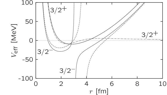
Figure 2: Effective (interaction + centrifugal) potentials corresponding to the wave functions of Fig. 1. The $3/2^{-}$ potentials have an $\ell=1$ centrifugal term and a singularity around 3-4 fm; the $3/2^{+}$ potentials have an $\ell=2$ centrifugal term and are regular. The dash-dotted line indicates the potential corresponding to the phenomenological $3/2^{+}$ wave function.

VII Alternative expressions for the width

Let us now return to the expression for the decay width and establish a link with known results. In Refs. Gurvitz and Kalbermann (1987); Gurvitz (1988); Gurvitz et al. the spatial derivatives were evaluated using a special form for $V(r)$ and $V_{00}(r)$. In those references these auxiliary potentials were chosen such that the total potential for $\phi_{\mathrm{r}0}(r)$ was constant outside a given radius and the one for $\phi_{\mathrm{r}E_{0}}(r)$ was constant inside. In Refs. Gurvitz and Kalbermann (1987); Gurvitz (1988) the separation radius is at the maximum of the potential barrier, whereas in Ref. Gurvitz et al. the advantage of using a radius of the order of the nuclear range (our $r_{0}$) is pointed out. For this last case, the width is then given by

$$\Gamma_{0}\approx 2\pi\left[\frac{\hbar^{2}\alpha}{2m_{k}(r_{0})}\right]^{2}|\phi_{\mathrm{r}0}(r_{0})\phi_{\mathrm{r}E_{0}}(r_{0})|^{2},$$ (44)

where $\alpha=\sqrt{2m_{k}(r_{0})[V(r_{0})-E_{0}]/\hbar^{2}}$.

An alternative approach is to exploit the Wronskian form of Eqs. (41) or (42). If $V(r)$ is zero for radii less than the outer turning point and $V_{00}(r)$ zero for radii greater than the inner turning point then there is a region where $\phi_{\mathrm{r}0}(r)$ and $\phi_{\mathrm{r}E_{0}}(r)$ satisfy the same differential equation. If the potential is local the Wronskian is a constant. Assuming a thick barrier, there will be a region where $\phi_{\mathrm{r}0}(r)$ is an irregular Coulomb function, the regular Coulomb function having decayed away, and where $\phi_{\mathrm{r}E_{0}}(r)$ is a regular Coulomb function, the irregular Coulomb function having decayed away. All that is required is to determine the proportionality constants. These have a simple expression for a constant effective mass $m_{k}(r)=m$: for $\phi_{\mathrm{r}E_{0}}(r)$ we have $\phi_{\mathrm{r}E_{0}}(r)=\sqrt{2m/\hbar^{2}k_{0}\pi}F(k_{0}r)$, with $k_{0}=\sqrt{2mE_{0}/\hbar^{2}}$, while for $\phi_{\mathrm{r}0}(r)$ the proportionality constant can be written as $\phi_{\mathrm{r}0}(r_{0})/G(k_{0}r_{0})$. Here $F(k_{0}r)$ and $G(k_{0}r)$ are the regular and irregular Coulomb functions respectively, the Wronskian of which equals $-k_{0}$. The resulting width is then, as in Ref. Gurvitz et al. ,

$$\Gamma_{0}\approx\frac{\hbar^{2}k_{0}}{m}|\phi_{\mathrm{r}0}(r_{0})/G(k_{0}r_{0})|^{2}.$$ (45)

This can be simplified further. The wave function $\phi_{\mathrm{r}0}(r)$ is normalized to the appropriate spectroscopic factor, $S_{0}$. We can also consider the true scattering wave function at resonance, $\phi^{\rm true}_{\mathrm{r}0}(r)$. In the interior it will behave like $\phi_{\mathrm{r}0}(r)$ while in the exterior region it will behave like $G(k_{0}r)$. Normalizing it to $G(k_{0}r)$ in the exterior region we obtain for the width:

$$\Gamma_{0}\approx\frac{S_{0}\hbar v_{0}}{\int_{0}^{r_{\mathrm{t}}}dr|\phi^{\rm true}_{\mathrm{r}0}(r)|^{2}},$$ (46)

where $v_{0}=\hbar k_{0}/m$ is the asymptotic velocity. The exact value of the upper limit on the integral is not crucial and we take it to be the outer turning point (see numerical justification below).

Equation (46) can also be derived in a more transparent way (see also Refs. Breit (1959); Iliadis (1997)). Consider the Schrödinger-like equation $[H(E)-E]\phi(\mathbf{r},E)=0$ for the overlap function. Since the effective one-body equation we have been considering can depend on the energy we keep an explicit energy dependence in the Hamiltonian. Differentiating this equation with respect to $E$ we find

$$[H(E)-E]\frac{\partial\phi(\mathbf{r},E)}{\partial E}=\left[1-\frac{\partial H(E)}{\partial E}\right]\phi(\mathbf{r},E).$$ (47)

Next we multiply by $\phi^{*}(\mathbf{r},E)$ and integrate up to some radius $r_{l}$. If $H(E)$ is not hermitian then $\phi^{*}(\mathbf{r},E)$ should be replaced by the time reversed state. If the potential is local in the vicinity of $r_{l}$ we can integrate by parts on the left hand side. Assuming spherical symmetry, this gives us

$$-\frac{\hbar^{2}}{2m_{k}(r_{l})}\left[\phi^{*}_{\mathrm{r}}(r_{l},E)\frac{\partial\phi_{\mathrm{r}}^{\prime}(r_{l},E)}{\partial E}-\phi^{\prime*}_{\mathrm{r}}(r_{l},E)\frac{\partial\phi_{\mathrm{r}}(r_{l},E)}{\partial E}\right]$$

$$\hskip 85.35826pt=\int_{0}^{r_{l}}dr\phi_{\mathrm{r}}^{*}(r,E)\left[1-\frac{\partial H_{\mathrm{r}}(E)}{\partial E}\right]\phi_{\mathrm{r}}(r,E),$$ (48)

where the prime denotes a partial derivative with respect to $r$ and $H_{\mathrm{r}}(E)$ is the radial Hamiltonian. If we take $r_{l}$ to be outside the range of nuclear force, $\phi_{\mathrm{r}}(r,E)$ can be written as

$$\phi_{\mathrm{r}}(r,E)\mathop{\approx}_{r>r_{0}}\cos{\delta(E)}F(kr)+\sin{\delta(E)}G(kr).$$ (49)

At a narrow resonance the phase shift $\delta(E)$ will be rapidly varying so we expect that the largest part of the energy dependence will come from the phase shift and not from the Coulomb functions. The energy dependence of the Coulomb functions will be minimized if the radius is chosen to be near the outside turning point. For example, for large $r$ the regular Coulomb function will have a $\sin(kr)$ dependence. Differentiating with respect to $E$ will give $r(dk/dE)\cos(kr)$, which diverges for large $r$. As $r$ decreases to the turning point this asymptotic form for the wave function breaks down. However a similar argument using exponentials holds inside the turning points. Thus near the outside turning point we have

$$\frac{\partial\phi_{\mathrm{r}}(r,E)}{\partial E}\approx\frac{d\delta(E)}{dE}[-\sin{\delta(E)}F(kr)+\cos{\delta(E)}G(kr)].$$ (50)

We have checked this relation numerically for Woods-Saxon plus Coulomb potentials and verified that for widths less then 15 KeV the error does not exceed 3%. That the radius should be chosen near the outer turning point was also confirmed numerically. The Wronskian relation can now be written as

$$\frac{\hbar^{2}k}{2m_{k}(r_{\mathrm{t}})}\frac{d\delta(E)}{dE}\approx\int_{0}^{r_{\mathrm{t}}}dr\phi_{\mathrm{r}}^{*}(r,E)\left[1-\frac{\partial H_{\mathrm{r}}(E)}{\partial E}\right]\phi_{\mathrm{r}}(r,E),$$ (51)

where we have taken $r_{l}=r_{\mathrm{t}}$ to be the outside turning point radius.

At the resonant energy we expect the energy variation of the phase shift to be a maximum so the resonance energy occurs when $\int_{0}^{r_{\mathrm{t}}}dr\phi^{*}_{\mathrm{r}}(r,E)\left[1-\frac{\partial H_{\mathrm{r}}(E)}{\partial E}\right]\phi_{\mathrm{r}}(r,E)$ is a maximum. At the resonance energy $d\delta(E_{0})/dE=2/\Gamma_{0}$, and we have

$$\Gamma_{0}\approx\frac{\hbar v_{0}}{\int_{0}^{r_{\mathrm{t}}}dr\phi^{*}_{\mathrm{r}}(r,E_{0})\left[1-\frac{\partial H_{\mathrm{r}}(E_{0})}{\partial E}\right]\phi_{\mathrm{r}}(r,E_{0})}\;,$$ (52)

where now $v_{0}=\hbar k_{0}/m$ is the asymptotic value of the velocity. For bound states the spectroscopic factor can be written as $S_{0}=\left[\int_{0}^{\infty}dr\phi^{*}_{\mathrm{r}}(r)\phi_{\mathrm{r}}(r)\right]/\left\{\int_{0}^{\infty}dr\phi^{*}_{\mathrm{r}}(r)\left[1-\frac{\partial H_{\mathrm{r}}(E)}{\partial E}\right]\phi_{\mathrm{r}}(r)\right\}$ (see Ref. Wegmann (1969)), which does not depend on the specific normalization of the overlap function $\phi(\mathbf{r})$. By extending this relation to define the spectroscopic factor for resonant states, we recover Eq. (46).

We finally note that the expression (52) of the width is independent of the choice of $\phi_{\mathrm{r}}(r,E)$ or $\bar{\phi}_{\mathrm{r}}(r,E)$. Its denominator can be rewritten as

$$D=\int_{0}^{r_{\mathrm{t}}}dr\phi^{*}_{\mathrm{r}}(r,E)\left\{\frac{\partial}{\partial E}\left[E-H_{\mathrm{r}}(E)\right]\right\}\phi_{\mathrm{r}}(r,E).$$ (53)

The bar-ed amplitudes are defined as $\bar{\phi}(\mathbf{r},E)=\int d\mathbf{r}\;{\cal N}(\mathbf{r},\mathbf{r}^{\prime})^{-1/2}\phi(\mathbf{r},E)$ and a corresponding expression for the Hamiltonian is $\bar{H}(E)={\cal N}^{1/2}\left[H(E)-E\right]{\cal N}^{1/2}+E$. Thus the denominator is invariant under this transformation, as well as under a general transformation with an arbitrary power of $\cal N(\mathbf{r},\mathbf{r}^{\prime})$. All that matters is that $H_{\mathrm{r}}(E)$ and $\phi_{\mathrm{r}}(r,E)$ are consistent with one another. These wave functions are phase equivalent and any of them can be used.

VIII Discussion

We have embedded the elegant Gurvitz-Kalbermann approach of proton emission Gurvitz and Kalbermann (1987); Gurvitz (1988); Gurvitz et al. into a full many-body picture. We have reduced the formalism to an effective one-body problem and demonstrated that the decay width can be expressed in terms of a one-body matrix element multiplied by a normalization factor. At first sight, this result agrees with the standard procedure for extracting spectroscopic factors from measurements via dividing an experimental width by a calculated single-particle width (see, for example, Ref. Åberg et al. (1997)). The present work, however, clearly demonstrates that this procedure for determining spectroscopic factors is only valid if the phenomenological potential used to generate the single-particle width corresponds to the potential in ${\cal H}_{\cal M}$ [see Eqs. (32) and (33)]. It is not a priori clear that this is actually the case. In fact, the authors of Refs. Varga and Lovas (1991); Lovas et al. (1998) (and prior to that the authors of Ref. Fliessbach and Mang (1976)) have argued strongly that the phenomenological potential approximates the potential in $\bar{\cal H}$ [see Eq. (29)]. While the studies of Refs. Varga and Lovas (1991); Lovas et al. (1998) were carried out for alpha decay, the arguments given there can be carried over to a description of the proton emission process. Furthermore, Eq. (52) suggests that $\int_{0}^{r_{t}}dr\phi^{*}_{\mathrm{r}}(r)\left[1-\frac{\partial H_{\mathrm{r}}(E)}{\partial E}\right]\phi_{\mathrm{r}}(r)$ is the appropriate observable that can be extracted from proton emission experiments.

Besides the ambiguity regarding whether the standard spectroscopic factor or an auxiliary normalization is extracted from the experimental procedure, it has been demonstrated that constructing a reliable phenomenological potential is non-trivial. The situation is quite complicated since the interaction with the nuclear medium strongly depends on the initial state of the ejected proton. For states with a clear core-plus-particle structure (i.e., with a large spectroscopic factor), traditional phenomenological potentials seem to provide good approximations to the nuclear mean field and spectroscopic factors can be determined from proton emission studies. In this case, the spectroscopic factor extracted from the experiment can be safely compared to the results of nuclear many-body calculations (note also that for large $S_{0}$ values, $S_{0}$ and $\bar{S}_{0}$ are approximately equal Escher and Jennings (2002) and the distinction between the two approaches discussed here becomes irrelevant).

For weak states, which have a more complicated many-body structure, standard phenomenological potentials do not give a proper approximation to the nuclear medium, as shown by the radial shape of the 3/2^- states in Fig. 2. Also, as discussed in Ref. Escher and Jennings (2002), the dependence of the spectroscopic factor on the energy derivative of the effective one-body Hamiltonian implies that the nuclear medium must be strongly energy dependent. This feature, which is missing in most phenomenological optical potentials, is also confirmed by the numerical results displayed in Fig. 2. Thus for weak states simple potential models are probably not valid for either $\phi(\mathbf{r})$ or $\bar{\phi}(\mathbf{r})$. States that are neither weak nor strong will also have to be dealt with on a case by case basis.

Since $\phi(\mathbf{r})$ and $\bar{\phi}(\mathbf{r})$ are identical for large radii they are phase equivalent and elastic scattering experiments cannot distinguish between them. We conclude that additional experimental input, together with an accurate derivation of the optical potential based on first principles, is required in order to resolve the question regarding which one-body Hamiltonian is most appropriately approximated by a phenomenological model.