Nuclear Isospin Diffusivity

Abstract

The isospin diffusion and other irreversible phenomena are discussed for a two-component nuclear Fermi system. The set of Boltzmann transport equations, such as employed for reactions, are linearized, for weak deviations of a system from uniformity, in order to arrive at nonreversible fluxes linear in the nonuniformities. Besides the diffusion driven by a concentration gradient, also the diffusion driven by temperature and pressure gradients is considered. Diffusivity, conductivity, heat conduction and shear viscosity coefficients are formally expressed in terms of the responses of distribution functions to the nonuniformities. The linearized Boltzmann-equation set is solved, under the approximation of constant form-factors in the distribution-function responses, to find concrete expressions for the transport coefficients in terms of weighted collision integrals. The coefficients are calculated numerically for nuclear matter, using experimental nucleon-nucleon cross sections. The isospin diffusivity is inversely proportional to the neutron-proton cross section and is also sensitive to the symmetry energy. At low temperatures in symmetric matter, the diffusivity is directly proportional to the symmetry energy.

I INTRODUCTION

The availability of beams largely differing in isospin content in nuclear reactions has dramatically increased interest in phenomena associated with the variation of that content. In the context of peripheral reactions, this includes interest in changes of the nuclear density profiles with the isospin content. In central reactions, the attention has focussed, in particular, on the dependence of isospin symmetry energy on density. The determination of that dependence would permit an extrapolation of the nuclear equation of state to the neutron matter limit lat01 . The isospin asymmetry has been used in central reactions for projectile-target tagging in the investigation of stopping Rami99 .

This paper deals with the irreversible transport of isospin and other quantities in a nuclear system, as pertinent for reactions, for small deviations from equilibrium. In that limit, the irreversible transport acquires universal features and is characterized in terms of transport coefficients, that include the isospin-diffusion coefficients. The coefficients are derived here for the dynamics described in terms of a Boltzmann equation set such as used in reaction simulations Bertsch ; Aichelin . The main diffusion coefficient or diffusivity, characterizing isospin diffusion driven by the gradient of asymmetry, is evaluated using free neutron-proton cross sections. In the past, other transport coefficients, viscosity and heat conductivity, have been investigated for nuclear matter Tomonaga ; gal79 ; PD84 ; hak92 ; hak93 . It was subsequently found that conclusions from comparisons of reaction simulations to data on stopping can be universally formulated in terms of the nuclear viscosity dan02 . It is hoped that the diffusivity can be of such utility as that other coefficient, for the systems with a varying isospin content.

The past studies of irreversible linear transport for nuclear matter were primarily directed at momentum and energy. Tomonaga Tomonaga and Galitskii et al. gal79 obtained the low- and high-temperature limits for the shear viscosity and heat conductivity. Danielewicz PD84 derived results for those coefficients valid in a wide range of nuclear densities and temperatures. Hakim and Mornas hak93 studied different transport coefficients within the Walecka model following the relaxation-time approximation.

Our derivation of diffusion coefficients follows the general strategy of Chapman and Enskog Chapman , but here for a Fermi system, with inclusion of mean-field effects such as appropriate for a nuclear system. In the next section, we discuss the diffusion coefficient concept qualitatively and make simple estimates for the nuclear matter. The modification of the Boltzmann equation to extend it to fermions has been first discussed by Uhlenbeck and Uehling ueh33 ; ueh34 . In Sec. III, we formally solve the set of Boltzmann equations for a binary system of fermions to find thermodynamic fluxes driven by specific thermodynamic forces and to find general but formal expressions for the diffusion and other transport coefficients. The transport coefficients have been (as we found) first considered for fermions by Hellund and Uhlenbeck hel39 ; compared to them, our notation here adheres more to what is now customary for nuclear reactions. Closely related to the diffusivity is the electrical conductivity that is included in our considerations. In Sec. IV, we obtain more specific results for the coefficients on assuming deviations from equilibrium suggested by the Boltzmann equation set, for specific thermodynamic forces present. Numerical results for the coefficients are obtained in Sec. V, using free NN cross sections. We also estimate there the pace of isospin equilibration in reactions. We summarize our results in Sec. VI. More technical mathematical details and some reference information are provided in five appendices. In sequence, these appendices are devoted to the definitions of macroscopic quantities, the continuity equations, the continuity equations for an ideal fluid, the transformations in the driving force for diffusion and to the algebra of collision brackets.

II Diffusion in a Binary System

Diffusion and other irreversible transport processes occur when a system is brought out of equilibrium. The direction of those processes is to bring the system back to the equilibrium. For small perturbations, in terms of constraints that may be set externally, the system response is linear in the perturbation. The coefficient of proportionality between the induced flux and the perturbation is the transport coefficient.

In a multicomponent system with no net mass flow, irreversible particle flows result if particle concentrations are nonuniform. For $N$ components, there are $N-1$ independent flows and $N-1$ independent concentrations (since the concentrations need to sum up to 1). The flows are then related to the gradients of the concentrations with an $(N-1)\times(N-1)$ matrix of diffusion coefficients. In a binary system, only a single coefficient of diffusion, or diffusivity, relates the irreversible particle flow to the nonuniformity in concentration. However, as we shall see, nonuniformities in other quantities than concentration, can induce a dissipative particle flow as well.

Our focus, obviously, is the binary system of neutrons and protons. However, for the sake of utility of the results elsewhere and for the ability to examine various limits, we shall consider a general two-component system of fermions. An extension of those results to bosons, outside of a condensation, will be trivial.

The two components will be denoted 1 and 2. Then, for the particle $i$, the density is $n_{i}=N_{i}/{\mathcal{V}}$, where $N_{i}$ is the particle number in some infinitesimal volume ${\mathcal{V}}$. With net density $n=n_{1}+n_{2}$, the particle concentration for 1 is $\nu=n_{1}/n$ and for 2 it is $1-\nu=n_{2}/n$. Moreover, with $m_{i}$ representing the mass of particle $i$, the net mass density is $\rho=\rho_{1}+\rho_{2}=m_{1}\,n_{1}+m_{2}\,n_{2}$, and the mass concentration for $i$ is $c_{i}=m_{i}\,n_{i}/\rho$. The differential particle concentration is $\delta=(n_{1}-n_{2})/n$. The different concentrations are obviously related and thus we have $\nu=(1+\delta)/2$ and $c_{1}=m_{1}\,(1+\delta)/(m_{1}\,(1+\delta)+m_{2}\,(1-\delta))$. Later in the paper, we shall primarily use the differential concentration $\delta$ as an independent variable.

The dissipative particle flows ${\bf\Gamma}_{i}$ are defined relative to the local mass velocity $\underline{\bf v}$,

$${\bf\Gamma}_{i}=n_{i}\,(\underline{\bf v}_{i}-\underline{\bf v})\,,$$ (1)

where $\underline{\bf v}_{i}$ is the local velocity of $i$’th component and

$$\underline{\bf v}=(\rho_{1}\,\underline{\bf v}_{1}+\rho_{2}\,\underline{\bf v}_{2})/\rho\,.$$ (2)

We might consider other flows such as defined relative to the local particle velocity, but those flows are combinations of ${\bf\Gamma}_{1}$ and ${\bf\Gamma}_{2}$. Moreover, even ${\bf\Gamma}_{1}$ and ${\bf\Gamma}_{2}$ are redundant and we might just use ${\bf\Gamma}_{1}$ as an independent flow with the flow of 2, as easily seen, given by ${\bf\Gamma}_{2}=-m_{1}\,{\bf\Gamma}_{1}/m_{2}$. Another option might be to use as independent the differential flow defined as

$${\bf\Gamma}_{\delta}={\bf\Gamma}_{1}-{\bf\Gamma}_{2}\,.$$ (3)

If the system is at uniform pressure and temperature, but there is a small concentration gradient present, the fluxes develop linear in the gradient, enabling us to write, e.g.

$${\bf\Gamma}_{1}=-n\,D_{1}\,\frac{\partial\nu}{\partial{\bf r}}\hskip 20.00003pt\mbox{and}\hskip 20.00003pt{\bf\Gamma}_{2}=-n\,D_{2}\,\frac{\partial(1-\nu)}{\partial{\bf r}}\,.$$ (4)

These are so-called Fick’s laws. Notably, the stability of an equilibrium state requires $D_{i}>0$. Since $m_{1}\,{\bf\Gamma}_{1}+m_{2}\,{\bf\Gamma}_{2}=0$, we have $m_{1}\,D_{1}=m_{2}\,D_{2}$. For the differential flow, we have

$${\bf\Gamma}_{\delta}=-n\,D_{1}\frac{\partial\nu}{\partial{\bf r}}+n\,D_{2}\,\frac{\partial(1-\nu)}{\partial{\bf r}}=-n\,D_{\delta}\,\frac{\partial\delta}{\partial{\bf r}}\,.$$ (5)

Here, the differential coefficient is $D_{\delta}=(D_{1}+D_{2})/2$.

So far, we assumed a system at a uniform pressure and temperature, with just concentration changing with position. If the variations in a system are more complex, other nonequilibrium forces than the concentration gradient can drive the diffusion. This will be explored later in the paper. General guidance regarding the forces which can contribute is provided by the Curie principle. This principle exploits symmetry and states that the driving forces must have the same tensor rank and parity as the flux they generate.

For the system of neutrons and protons, the differential concentration $\delta$ becomes a concentration of the isospin and the differential flow becomes the isospin flow, $\Gamma_{\delta}\equiv\Gamma_{I}$. Moreover, the differential diffusion coefficient becomes an isospin diffusion coefficient, $D_{\delta}\equiv D_{I}$, and for equal masses we expect $D_{I}=D_{p}=D_{n}$.

It is popular to relate the concept of a diffusion coefficient to a diffusion equation. Indeed, if we consider a uniform system of protons and neutrons at rest, but with the nucleon concentration changing in space, then, from the continuity equation for the differential density

$$\frac{\partial\left(n\,\delta\right)}{\partial t}=-\nabla\cdot{\bf\Gamma}_{I}\,,$$ (6)

we get the familiar equation

$$\frac{\partial\delta}{\partial t}=D_{I}\,\nabla^{2}\delta\,.$$ (7)

Here, for $D_{I}$, we have assumed a weak dependence on the concentration $\delta$.

Before turning to a derivation of rigorous results for the diffusion and other transport coefficients, it may be instructive to produce simple mean-free-path estimates for those coefficients. Let us consider components of equal mass (the mass then becomes a simple normalization coefficient in density that may be factored out) and consider the gradient of concentration along the $x$ axis, in the medium at rest. If we take the three coordinate axes, then 1/6 of all particles will be primarily moving along one of those axes in the positive or negative direction, with an average thermal velocity $\underline{V}=\sqrt{3T/m}$, for the distance of the order of one mean free path $\lambda$, without a collision. Considering the particles 1 moving through the plane at $x=0$, they will be reflecting density at a distance $\lambda$ away. Including the particles moving up and down through the plane, we find for the flux

$$\Gamma_{1}\approx\frac{1}{6}\left(n_{1}(x-\lambda)-n_{1}(x+\lambda)\right)\,\underline{V}\approx-\frac{1}{3}\lambda\,\underline{V}\,\frac{\partial n_{1}}{\partial x}\,.$$

With (4), we then get for the diffusion coefficient

$$D\sim\frac{1}{3}\lambda\,\underline{V}\sim\frac{1}{n\,\sigma}\sqrt{\frac{T}{3m}}\,,$$ (8)

with $\lambda\sim 1/(n\,\sigma)$. A more thorough investigation shows that it is the cross section $\sigma_{12}$ for interaction between the two species that enters the diffusion coefficient.

Let us now evaluate the magnitude of the isospin diffusion coefficient. At temperature $T\sim 60$ MeV and normal density $n_{0}=0.16$ fm^-3, with $\sigma_{np}\sim 40$ mb, we find $D_{I}\sim 0.2$ fm$\,c$. We will see this to be in a rough agreement with thorough calculations.

Similarly to the above, one could employ the mean-free path arguments to determine the better investigated coefficients: shear-viscosity $\eta$ and heat conduction $\kappa$. One finds $\eta\sim\frac{1}{3}n\,m\,\underline{V}\,\lambda$ and $\kappa\sim\frac{1}{3}n\,\underline{V}\,\lambda\,c_{V}$, where $c_{V}$ is the specific heat per particle. For $T\sim 60$ MeV and $\sigma\sim 40$ mb, we find $\eta\sim 30$ MeV/(fm² c) and $\kappa\sim 0.06$ c/fm². Up to factors, the shear viscosity and heat conduction coefficients play the role of diffusion coefficients in the diffusion equation for velocity vorticity and in the heat conduction Fourier equation identical in form to the diffusion equation.

In the estimates above, we just considered the free motion of particles in-between collisions. If self-consistent mean fields produced by the particles depend on concentration, then this dependence, on its own, contributes to the diffusion. In the case of nuclear matter, the interaction energy per nucleon may be well approximated in the form quadratic in isospin asymmetry, $E_{I}^{v}=a_{I}^{v}\,\delta^{2}$, where $\delta=(n_{p}-n_{n})/n$ and $a_{I}^{v}$ is the interaction contribution to the asymmetry coefficient $a_{I}$. At normal density, the coefficient is $a_{I}^{v}\approx 14$ MeV. The naive expectation for two-body interactions is that $a_{I}^{v}$ is linear in density. At constant net density, the quadratic dependence of the interaction energy on $\delta$ leads to the force ${\bf F}_{p,n}=\mp\frac{4\,a_{I}^{v}}{n}\,\frac{\partial n_{p}}{\partial{\bf r}}$, of opposite sign on protons and neutrons. The direction of the force for positive $a_{I}^{v}$ is to reduce nonuniformity in isospin. Under the influence of this force, a proton accelerates for a typical time between collisions $\Delta t=\lambda/\underline{V}$ and then, in a collision, resets its velocity. The described polarization effect augments then the proton flow by

$$\Delta{\bf\Gamma}_{p}=n_{p}\,\Delta\underline{\bf v}_{p}=-\frac{4\,a_{I}^{v}\,n_{p}}{n}\,\frac{\lambda}{2\,m\,\underline{V}}\frac{\partial n_{p}}{\partial{\bf r}}\,.$$ (9)

In comparing with (II), after correcting for the local center of mass motion, we find that the polarization increases the diffusion coefficient by

$$D_{I}^{\prime}\sim(1-\delta^{2})\frac{a_{I}^{v}}{T}\,D_{I}^{0}\,,$$ (10)

where $D_{I}^{0}$ represents the previous estimate in Eq. (8). It is apparent that the contribution of the polarization effect is negligible for temperatures $T\gg a_{I}^{v}$. However, at temperatures comparable to $a_{I}^{v}$, the contribution could be significant; notably, at those temperatures Fermi effects also need to play a role.

The isospin diffusion induced by mechanical forces has analogy in an electric current induced by the electric fields. Indeed, for large enough systems, the Coulomb interactions can contribute currents altering the concentration and, for completeness, we evaluate the conductivity $\sigma_{E}$ for nuclear matter, relating the isospin flux to the electric field,

$${\bf\Gamma}_{I}=\sigma_{E}\,{\bf\mathcal{E}}\,,$$ (11)

where ${\bf\mathcal{E}}$ is the local electric field.

III Fluxes from the Boltzmann Equation Set

III.1 Coupled Boltzmann Equations

The two components of the binary system will be described in terms of the quasiparticle distribution functions $f_{i}({\bf p},{\bf r},t)$. The local macroscopic quantities $h({\bf r},t)$ are expressed as momentum integrals of $f$,

$$h({\bf r},t)=\frac{g}{(2\pi\hbar)^{3}}\int{d{\bf p}}\,{\chi({\bf p})f({\bf p},{\bf r},t)}\,,$$ (12)

where $g$ is the intrinsic degeneracy factor. Different standard expressions for macroscopic quantities in terms of $f$, such as pressure and heat flow, are listed in the Appendix A.

The components are assumed to follow the set of coupled fermion Boltzmann equations,

$${\frac{\partial f_{i}}{\partial t}}+\frac{\bf p}{m_{i}}\cdot\frac{\partial{f_{i}}}{\partial{\bf r}}+{\bf F}_{i}\cdot\frac{\partial{f_{i}}}{\partial{\bf p}}=J_{i}\,.$$ (13)

The terms on the l.h.s. account for the changes in $f_{i}$ due to the movement of quasiparticles and their acceleration under the influence of mean-field and external forces, included in ${\bf F}_{i}$, while the r.h.s. accounts for the changes in $f_{i}$ due to collisions. In the following, we shall often denote the l.h.s. of a Boltzmann equation as ${\mathcal{D}}_{i}$. With $d\sigma/d\Omega$ and $v^{*}$ representing the differential cross section and relative velocity, respectively, the collision integral for particle 1 is

$$J_{1}=J_{11}+J_{12} = \frac{g}{2(2\pi\hbar)^{3}}\int d^{3}p_{1a}\,d\Omega^{\prime}\,v^{*}\left(\frac{d\sigma_{11}}{d\Omega}\right)\,\left(\tilde{f}_{1}\,\tilde{f}_{1a}\,f_{1}^{\prime}\,f_{1a}^{\prime}-{f}_{1}\,{f}_{1a}\,\tilde{f}_{1}^{\prime}\,\tilde{f}_{1a}^{\prime}\right)$$ (14)

$$+\frac{g}{(2\pi\hbar)^{3}}\int d^{3}p_{2}\,d\Omega^{\prime}\,v^{*}\left(\frac{d\sigma_{12}}{d\Omega}\right)\,\left(\tilde{f}_{1}\,\tilde{f}_{2}\,f_{1}^{\prime}\,f_{2}^{\prime}-{f}_{1}\,{f}_{2}\,\tilde{f}_{1}^{\prime}\,\tilde{f}_{2}^{\prime}\right)\,.$$

Here, $\tilde{f}=1-f$ is the Pauli principle factor. The factor of $1/2$ in front of the first r.h.s. $J_{11}$ term, compared to the $J_{12}$ term, compensates for the double-counting of final states when integration is done over the full spherical angle in scattering of identical particles. The subscript $a$ and the primes in combination with the particle subscripts $1$ and $2$ are used to keep track of incoming and outgoing particles for a collision. Other than in the context of particle components, such as here, the $1$ and $2$ subscripts will not be utilized in the paper. The collision integral $J_{2}$ for particles $2$ follows from (14) upon interchange of the indices $1$ and $2$. As it stands, the set of the Boltzmann equations (13), with (14), preserves the number of each species.

In the macroscopic quantities (12), the distribution function $f$ gets multiplied by the degeneracy factor $g$. When considering changes of macroscopic quantities (12) dictated by the Boltzmann equation (13), the changing distribution function $f$ continues to be multiplied by $g$. In the equation, the factor of $f$ for the other particle in the collision integral $J$ is accompanied by its own factor of $g$. As a consequence, in the variety of physical quantities we derive, the factor of $f$ is always accompanied by the factor of $g$, while, however, $\tilde{f}$ is not. To simplify the notation, in the derivations that follow, we suppress the factors of $g$, only to restore those factors towards the end of the derivations.

When the Boltzmann equation set is used to study the temporal changes of densities of the quantities conserved in collisions, i.e. number of species, energy and momentum, local conservation laws follow. Those conservation laws are discussed in Appendix B.

III.2 Strategy for Solving the Boltzmann Equation Set

Irreversible transport takes place when the system is brought out of equilibrium such as in effect of external constraints. Aiming at the transport coefficients, we shall assume that the deviations from the equilibrium are small, of the order of some parameter $\epsilon$ that sets the scale for temporal and spatial changes in the system. Then the distribution functions may be expanded in the power series in $\epsilon$ Chapman ; Liboff

$$f=f^{(0)}+f^{(1)}+f^{(2)}+\ldots\,,$$ (15)

where $f^{(k)}$ represent the consecutive terms of expansion and $f^{(0)}$ is the strict local equilibrium solution. The terms of expansion in $f$ may be nominally found by expanding the collision integrals in $\epsilon$, following (15), expanding, simultaneously, the derivative terms in the equations and by demanding a consistency,

$${\mathcal{D}}_{i}^{(1)}+{\mathcal{D}}_{i}^{(2)}+\ldots=J_{i}^{(0)}+J_{i}^{(1)}+J_{i}^{(2)}+\ldots\,.$$ (16)

Here, we recognize that the derivatives, themselves, bring in a power of $\epsilon$ into the equations and, thus, the derivative series starts with a first order term in $\epsilon$.

While we nominally included the zeroth-order term in the expansion of the collision integral $J_{i}$, the integral vanishes for the equilibrium functions

$$f_{j}^{(0)}=\frac{1}{\exp{\left(\frac{\frac{({\bf p}-m_{j}\,{\bf v})^{2}}{2m_{j}}-\mu_{j}}{T}\right)}+1}\,,$$ (17)

where $\mu_{j}$, ${\bf v}$ and $T$ are the local kinetic chemical potential, velocity and temperature which are functions of ${\bf r}$ and $t$, consistent with the Euler equations (84). Notably, the vanishing of the collision integrals is frequently exploited in deriving the form of the equilibrium functions, leading to the requirement that $f_{j}/\tilde{f}_{j}$ is given by the exponential of a linear combination of the conserved quantities. In the context of specific transport coefficients, the boundary conditions for the Euler equations (84) may be chosen to generate just those irreversible fluxes, and forces driving those fluxes, that are of interest.

The equation set (16) can be solved by iteration, order by order in $\epsilon$, requiring

$${\mathcal{D}}_{i}^{(k)}=J_{i}^{(k)}\,.$$ (18)

Thus, $f_{j}^{(0)}$ may be introduced into ${\mathcal{D}}_{i}$, producing ${\mathcal{D}}_{i}^{(1)}$ and allowing to find $f_{j}^{(1)}$. Next, inserting $f_{j}^{(1)}$ into ${\mathcal{D}}_{i}$ yields ${\mathcal{D}}_{i}^{(2)}$ that allows to find $f_{j}^{(2)}$ and so on.

For finding the coefficients of linear transport, only one iteration above is necessary, since $f_{i}^{(1)}$, as linear in gradients, yield dissipative fluxes that are linear in those gradients. The local equilibrium functions on its own produce no dissipative fluxes, as the species local velocities ${\bf V}_{j}$ and heat flux ${\bf Q}$ vanish, while the kinetic pressure tensor $\overline{\overline{P}}$ is diagonal,

$$n_{i}\,{\bf V}_{i}^{(0)} = \int\frac{d^{3}p}{(2\pi\hbar)^{3}}\,\frac{{\bf p}}{m_{i}}\,f_{i}^{(0)}({\bf p},{\bf r},t)=0\,,$$ (19a)

$${\bf Q}^{(0)} = \sum_{j}\int\frac{d^{3}p}{(2\pi\hbar)^{3}}\,\frac{p^{2}}{2m_{j}}\,\frac{{\bf p}}{m_{j}}\,f_{j}^{(0)}({\bf p},{\bf r},t)=0\,,$$ (19b)

$$\overline{\overline{P}}^{(0)} = \sum_{j}\int\frac{d^{3}p}{(2\pi\hbar)^{3}}\,\frac{\overline{\overline{{\bf p}\,{\bf p}}}}{m_{j}}\,f_{j}^{(0)}({\bf p},{\bf r},t)=\frac{2}{3}\,n\,\underline{E}\,\overline{\overline{1}}\,,$$ (19c)

in the frame where the local velocity vanishes ${\bf v}({\bf r},t)=0$, with $\underline{E}$ representing the local kinetic energy per particle. The above fluxes reduce the local continuity equations to the ideal-fluid Euler equations.

III.3 Boltzmann Set in the Linear Approximation

We now consider the terms linear in derivatives around a given point, i.e. the case of $k=1$ in (18), for the Boltzmann equation set. On representing the distribution functions as $f_{j}=f_{j}^{(0)}+f_{j}^{(1)}$, we expand the collision integrals $J_{i}$, to get terms $J_{i}^{(1)}$ linear in $f_{j}^{(1)}$. Upon representing $f_{j}^{(1)}$ as $f_{j}^{(1)}=f_{j}^{(0)}\,\tilde{f}_{j}^{(0)}\,\phi_{j}$, we get for the $k=1$ $i=1$ version of (18):

$${\frac{\partial f_{1}^{(0)}}{\partial t}}+\frac{\bf p}{m_{1}}\cdot\frac{\partial{f_{1}^{(0)}}}{\partial{\bf r}}+{\bf F}_{1}\cdot\frac{\partial{f_{1}^{(0)}}}{\partial{\bf p}}=-I_{11}(\phi)-I_{12}(\phi)\,,$$ (20)

where

$$I_{ij}(\phi)=\frac{1}{1+\delta_{ij}}\int\frac{d^{3}p_{ja}}{(2\pi)^{3}}\,d\Omega^{\prime}\,v^{*}\left(\frac{d\sigma_{ij}}{d\Omega}\right)\,f_{i}^{(0)}\,f_{ja}^{(0)}\,{\tilde{f}_{i}^{(0)\prime}}\,{\tilde{f}_{ja}^{(0)\prime}}\,\left(\phi_{i}+\phi_{ja}-\phi_{i}^{\prime}-\phi_{ja}^{\prime}\right)\,,$$ (21)

and where we have utilized the property of the equilibrium functions

$$f_{i}^{(0)}\,f_{ja}^{(0)}\,{\tilde{f}_{i}^{(0)\prime}}\,{\tilde{f}_{ja}^{(0)\prime}}=\tilde{f}_{i}^{(0)}\,\tilde{f}_{ja}^{(0)}\,{{f}_{i}^{(0)\prime}}\,{{f}_{ja}^{(0)\prime}}\,.$$ (22)

The result for $i=2$, analogous to (20), is obtained through an interchange of the indices 1 and 2.

The l.h.s. of Eq. (20) contains the derivatives of equilibrium distribution functions with respect to $t$, ${\bf r}$ and ${\bf p}$. These derivatives can be expressed in terms of the parameters describing the functions (17), i.e. $\mu_{i}$, $T$ and ${\bf v}$. Through the use of the Euler equations (Appendix B) and equilibrium identities (Appendix C), moreover, the temporal derivatives may be eliminated to yield for the rescaled l.h.s. of (20)

$$\frac{T}{f_{1}^{(0)}\,\tilde{f}_{1}^{(0)}}\,{\mathcal{D}}^{(1)}=\left(\frac{p^{2}}{2m_{1}}-\frac{5}{3}\,\underline{E}\right)\frac{\bf p}{m_{1}\,T}\cdot\frac{\partial T}{\partial{\bf r}}+\frac{\mathring{\overline{\overline{\bf p\,p}}}}{m_{1}}:\overline{\overline{\frac{\partial}{\partial{\bf r}}{\bf v}}}+\frac{\bf p}{\rho_{1}}\cdot{\bf d}_{12}\,.$$ (23)

Here, a symmetrized traceless tensor is defined as $\mathring{\overline{\overline{\bf x\,y}}}=\frac{1}{2}\left(\overline{\overline{\bf x\,y}}+\overline{\overline{\bf y\,x}}\right)-\frac{1}{3}\left({\bf x}\cdot{\bf y}\right)\overline{\overline{1}}$, and

$${\bf d}_{12} = \frac{\rho_{1}\,\rho_{2}}{\rho}\left[\left(-\frac{{\bf F}_{1}}{{m_{1}}}+\frac{{\bf F}_{2}}{{m_{2}}}\right)+T\,\frac{\partial}{\partial{\bf r}}\left(\frac{\mu_{1}}{m_{1}\,T}-\frac{\mu_{2}}{m_{2}\,T}\right)+\frac{5}{3\,T}\left(\frac{\underline{E}_{1}}{m_{1}}-\frac{\underline{E}_{2}}{m_{2}}\right)\,{\frac{\partial T}{\partial{\bf r}}}\right]\,,$$ (24)

$$= \frac{\rho_{1}\,\rho_{2}}{\rho}\left[\left(-\frac{{\bf F}_{1}}{{m_{1}}}+\frac{{\bf F}_{2}}{{m_{2}}}\right)+\frac{\partial}{\partial{\bf r}}\left(\frac{\mu_{1}}{m_{1}}-\frac{\mu_{2}}{m_{2}}\right)+\left(\frac{s_{1}}{m_{1}}-\frac{s_{2}}{m_{2}}\right)\,\frac{\partial T}{\partial{\bf r}}\right]\,,$$

where $s_{i}$ is the entropy per particle for species $i$, $s_{i}=(5\underline{E}_{i}/3-\mu_{i})/T$. The result for species 2 in the Boltzmann equation is obtained by interchanging the indices 1 and 2 in Eqs. (23) and (24). Note that ${\bf d}_{21}=-{\bf d}_{12}$.

The representation (23) for the l.h.s. of the linearized Boltzmann equation (20) exhibits the thermodynamic forces driving the dissipative transport in a medium. Thus, we have the tensor of velocity gradients $\overline{\overline{\frac{\partial}{\partial{\bf r}}{\bf v}}}$ contracted in (23) with the tensor from particle momentum. The distortion of the momentum distribution associated with the velocity gradients gives rise to the tensorial dissipative momentum flux in a medium. As to the vectorial driving forces, they all couple to the momentum in (23) and they all can contribute to the vector fluxes in the medium, i.e. the particle and heat fluxes, as permitted by the Curie law. The criterion that we, however, employed in separating the driving vectors forces in (23) was that of symmetry under the particle interchange. When considering the diffusion in a binary system, with the two components flowing in opposite directions in a local frame, one expects the driving force to be of an opposite sign on the two species. On the other hand, in the case of the heat conduction, one expects the driving force to distort the distributions of the two species in a similar way in the same direction.

Regarding the antisymmetric driving force in (24), we may note that for conservative forces we have

$${\bf F}_{i}=-\frac{\partial}{\partial{\bf r}}U_{i}\,.$$ (25)

We can combine then the first with the second term on the r.h.s. of (24) by introducing the net chemical potentials $\mu_{i}^{t}=\mu_{i}+U_{i}$ and getting

$${\bf d}_{12}=\frac{\rho_{1}\,\rho_{2}}{\rho}\left[\frac{\partial}{\partial{\bf r}}\left(\frac{\mu_{1}^{t}}{m_{1}}-\frac{\mu_{2}^{t}}{m_{2}}\right)+\left(\frac{s_{1}}{m_{1}}-\frac{s_{2}}{m_{2}}\right)\,\frac{\partial T}{\partial{\bf r}}\right]\,.$$ (26)

For a constant temperature $T$, the driving force behind diffusion is the gradient of difference between the chemical potentials per unit mass, $\mu_{12}^{t}=\mu_{1}^{t}/m_{1}-\mu_{2}^{t}/m_{2}$, as expected from phenomenological considerations Landau . However, the temperature gradient can contribute to the diffusion as well, which is known as the thermal diffusion or Soret effect. We note that the vector driving forces in (23) vanish when the temperature and the difference of net chemical potentials per mass are uniform throughout a system.

Given the typical constraints on a system, it can be more convenient to obtain the driving forces in terms of the net pressure $P^{t}$, temperature $T$ and concentration $\delta$, rather than $\mu_{12}^{t}$ and $T$. Thus, on expressing the potential difference as $\mu_{12}^{t}=\mu_{12}^{t}(P^{t},T,\delta)$, we get

$$d\mu_{12}^{t}=\left(\frac{\partial\mu_{12}^{t}}{\partial P^{t}}\right)_{T,\delta}\,dP^{t}+\left(\frac{\partial\mu_{12}^{t}}{\partial T}\right)_{P^{t},\delta}\,dT+\left(\frac{\partial\mu_{12}^{t}}{\partial\delta}\right)_{P^{t},T}\,d\delta\,,$$ (27)

and

$${\bf d}_{12}=\frac{\rho_{1}\,\rho_{2}}{\rho}\,\left(\Pi_{12}^{P}\,{\bf\nabla}P^{t}+\Pi_{12}^{T}\,{\bf\nabla}{T}+\Pi_{12}^{\delta}\,{\bf\nabla}\delta\right)\,,$$ (28)

that we will utilize further on. The coefficient functions are

$$\Pi_{12}^{P} = \left(\frac{\partial\mu_{12}^{t}}{\partial P^{t}}\right)_{T,\delta}\,,$$ (29a)

$$\Pi_{12}^{T} = \left(\frac{\partial\mu_{12}^{t}}{\partial T}\right)_{P^{t},\delta}+\left(\frac{s_{1}}{m_{1}}-\frac{s_{2}}{m_{2}}\right)\,,$$ (29b)

$$\Pi_{12}^{\delta} = \left(\frac{\partial\mu_{12}^{t}}{\partial\delta}\right)_{P^{t},T}\,,$$ (29c)

and specific expressions for those functions in the nuclear-matter case are given in Appendix D. Notably, however, the concentration $\delta$ may not be a convenient variable in the phase transition region where the transformation between the chemical potential difference and $\delta$ is generally not invertible.

With the l.h.s. of the linearized Boltzmann set (20) linear in the driving forces exhibited on the r.h.s. of (23), and with the collision integrals linear in the deviation form-factors $\phi$, the form factors need to be linear in the driving forces,

$$\phi_{1} = -{\bf A}_{1}\cdot{\bf\nabla}T-\overline{\overline{B}}_{1}:\mathring{\overline{\overline{\bf\nabla v}}}-{\bf C}_{1}\cdot{\bf d}_{12}\,,$$

$$\phi_{2} = -{\bf A}_{2}\cdot{\bf\nabla}T-\overline{\overline{B}}_{2}:\mathring{\overline{\overline{\bf\nabla v}}}-{\bf C}_{2}\cdot{\bf d}_{12}\,,$$ (30)

where ${\bf A}$, $\overline{\overline{B}}$ and ${\bf C}$ do not depend on the forces. On inserting (30) into (20), we get the following equations, when keeping alternatively a selected exclusive driving force finite:

$$\frac{{\bf p}}{\rho_{1}\,T}\,f_{1}^{(0)}\,\tilde{f}_{1}^{(0)} = I_{11}({\bf C})+I_{12}({\bf C})\,,$$ (31a)

$$-\frac{{\bf p}}{\rho_{2}\,T}\,f_{2}^{(0)}\,\tilde{f}_{2}^{(0)} = I_{22}({\bf C})+I_{21}({\bf C})\,,$$ (31b)

when keeping ${\bf d}_{12}$,

$$\frac{\mathring{\overline{\overline{\bf p\,p}}}}{m_{1}\,T}\,f_{1}^{(0)}\,\tilde{f}_{1}^{(0)}=I_{11}(\overline{\overline{B}})+I_{12}(\overline{\overline{B}})\,,$$ (32)

and another one, with indices $1$ and $2$ interchanged, when keeping $\mathring{\overline{\overline{\bf\nabla v}}}$, and, finally,

$$\left(\frac{p^{2}}{2m}-\frac{5}{3}\underline{E}_{1}\right)\frac{\bf p}{m_{1}\,T^{2}}\,f_{1}^{(0)}\,\tilde{f}_{1}^{(0)}=I_{11}({\bf A})+I_{12}({\bf A})\,,$$ (33)

and another one, with $1$ and $2$ interchanged, when keeping ${\bf\nabla}T$ (while ${\bf d}_{12}=0$).

The linearized collision integrals $I_{ij}$ cannot change the tensorial character of objects upon which they operate. Moreover, the only vector that can be locally utilized in the object construction is the momentum ${\bf p}$. This implies, then, the following representation within the set (30):

$${\bf C}_{i} = c_{i}(p^{2})\,\frac{\bf p}{\rho_{i}}\,,$$ (34a)

$${\bf A}_{i} = a_{i}(p^{2})\left(\frac{{p}^{2}}{2m_{i}}-\frac{5}{3}\underline{E}_{i}\right)\,\frac{\bf p}{m_{i}\,T^{2}}\,,$$ (34b)

$$\overline{\overline{B}} = b_{i}(p^{2})\,\mathring{\overline{\overline{{\bf p}\,{\bf p}}}}\,.$$ (34c)

Here, the tensorial factors are enforced by construction. The factorization of the scalar factors is either suggested by the respective linearized Boltzmann equation or serves convenience later on. The unknown functions $a$, $b$ and $c$ can be principally found by inserting (34) into Eqs. (31)-(33). The resulting equations are, however, generally quite complicated and analytic solutions are only known in some special cases. In practical calculations, we shall contend ourselves with a power expansion for the unknown functions. It has been shown that any termination of the expansion will produce lower bounds for the transport coefficients and that the lowest terms yield a predominant contribution to the coefficients Chapman .

III.4 Formal Results for Transport Coefficients

Before solving Eqs. (31)-(33), we shall obtain formal results for the transport coefficients, assuming that solutions to (31)-(33) exist. We shall start with the diffusion. The velocity for species $1$ is

$$\underline{\bf V}_{1} = \frac{1}{n_{1}}\int\frac{d^{3}p}{(2\pi\hbar)^{3}}\,\frac{\bf p}{m_{1}}\,\delta f_{1}=\frac{1}{n_{1}}\int\frac{d^{3}p}{(2\pi\hbar)^{3}}\,\frac{\bf p}{m_{1}}\,\phi_{1}\,f_{1}^{(0)}\,\tilde{f}_{1}^{(0)}$$ (35)

$$= T\int\frac{d^{3}p}{(2\pi\hbar)^{3}}\,\phi_{1}\,\left[I_{11}({\bf C})+I_{12}({\bf C})\right]$$

$$= -{\bf\nabla}T\,\frac{T}{3}\int\frac{d^{3}p}{(2\pi\hbar)^{3}}\,{\bf A}_{1}\cdot\left[I_{11}({\bf C})+I_{12}({\bf C})\right]$$

$$-{\bf d}_{12}\,\frac{T}{3}\int\frac{d^{3}p}{(2\pi\hbar)^{3}}\,{\bf C}_{1}\cdot\left[I_{11}({\bf C})+I_{12}({\bf C})\right]\,,$$

where we have utilized (30) and (34). The contribution of a tensorial driving force to the vector flow drops out under the integration over momentum, as required by the Curie principle. With a result for $\underline{\bf V}_{2}$ analogous to (35), we get for the difference of average velocities (utilized for the sake of particular symmetry between the components)

$$\underline{\bf V}_{1}-\underline{\bf V}_{2} = -{\bf\nabla}T\,\frac{T}{3}\,\Bigg{\{}\int\frac{d^{3}p}{(2\pi\hbar)^{3}}\,{\bf A}_{1}\cdot\left[I_{11}({\bf C})+I_{12}({\bf C})\right]$$ (36)

$$+\int\frac{d^{3}p}{(2\pi\hbar)^{3}}\,{\bf A}_{2}\cdot\left[I_{22}({\bf C})+I_{21}({\bf C})\right]\Bigg{\}}$$

$$-{\bf d}_{12}\,\frac{T}{3}\Bigg{\{}\int\frac{d^{3}p}{(2\pi\hbar)^{3}}\,{\bf C}_{1}\cdot\left[I_{11}({\bf C})+I_{12}({\bf C})\right]$$

$$+\int\frac{d^{3}p}{(2\pi\hbar)^{3}}\,{\bf C}_{2}\cdot\left[I_{22}({\bf C})+I_{21}({\bf C})\right]\Bigg{\}}$$

$$= -\frac{T}{3}\left(\{{\bf A},{\bf C}\}\,{\bf\nabla}T+\{{\bf C},{\bf C}\}\,{\bf d}_{12}\right)\,,$$

where the brace product $\{\cdot,\cdot\}$ is an abbreviation for the integral combinations of vectors ${\bf A}$ and ${\bf C}$, multiplying the driving forces. The brace product has been first introduced for a classical gas Chapman . The fermion generalization of the product and its properties are discussed in the Appendix E; see also hel39 .

The diffusion coefficient is best defined with regard to the most common conditions under which the diffusion might occur, i.e. at uniform pressure and temperature, but varying concentration. We have then, cf. (3),

$$\underline{\bf V}_{1}-\underline{\bf V}_{2}=\frac{\rho}{(m_{1}+m_{2})\,n_{1}\,n_{2}}\,{\bf\Gamma}_{\delta}=-\frac{\rho\,n\,m_{12}}{\rho_{1}\,\rho_{2}}\,D_{\delta}\,{\bf\nabla}\delta\,,$$ (37)

where $m_{12}$ is the reduced mass, $1/m_{12}=1/m_{1}+1/m_{2}$. Respectively, when $P^{t}$ and $T$ vary, with ${\bf d}_{12}$ given by (28), we write the r.h.s. of (36) as

$$\underline{\bf V}_{1}-\underline{\bf V}_{2}=-\frac{\rho\,n\,m_{12}}{\rho_{1}\,\rho_{2}}\,D_{\delta}\left({\bf\nabla}\delta+\frac{\Pi^{P}}{\Pi^{\delta}}\,{\bf\nabla}P^{t}+k_{T}\,{\bf\nabla}T\right)\,,$$ (38)

where, simplifying the notation, we dropped the subscripts $12$ on coefficients $\Pi$. The diffusion coefficient in the above is given by

$$D_{\delta}=\frac{T}{3m_{12}}\,\frac{\Pi^{\delta}}{n}\,\left(\frac{\rho_{1}\,\rho_{2}}{\rho}\right)^{2}\{{\bf C},{\bf C}\}\,,$$ (39)

and

$$k_{T}=\frac{\Pi^{T}}{\Pi^{\delta}}+\frac{1}{\Pi^{\delta}}\,\frac{\rho}{\rho_{1}\,\rho_{2}}\,\frac{\{{\bf A},{\bf C}\}}{\{{\bf C},{\bf C}\}}\,.$$ (40)

We can note that the expressions above contain $\Pi^{\delta}$ in denominators. Normally, positive nature of the derivative (29c) is ensured by the demand of the system stability. However, across the region of a phase transition the concentration generally changes while the chemical potentials generally do not, so that $\Pi^{\delta}=0$. While the coefficient $D_{\delta}$ above is the one we are after as the standard one in describing diffusion, in the phase transition region it can be beneficial to resort to the description of diffusion as responding to the gradient of the potential difference in (28). Notably, as explained in the Appendix E, the brace product $\{C,C\}$ in (39) is positive definite. This ensures the positive nature of $D_{\delta}$ away from the phase transition and, in general, ensures that, at a constant temperature, the irreversible asymmetry flux flows in the direction from a higher potential difference $\mu_{12}^{t}$ to lower.

As to the Soret effect, i.e. diffusion driven by the temperature gradient, described in (38)-(40), it has its counterpart in the heat flow driven by a concentration gradient, termed Dufour effect. Transport coefficients for counterpart effects are related through Onsager relations Groot that are also borne out by our results. The diffusion driven by pressure is rarely of interest, because of the usually short times for reaching the mechanical equilibrium in a system, compared to the equilibrium with respect to temperature or concentration. However, an irreversible particle flux may be further driven by external forces, such as due to an electric field ${\bf\mathcal{E}}$. With the flux induced by the field given by ${\bf\Gamma}_{\delta}=\sigma_{E}\,{\bf\mathcal{E}}$, where $\sigma_{E}$ is conductivity, with the first equality in (37), and with (36) and (24), we find for the conductivity

$$\sigma_{E}=\frac{T}{3m_{12}}\,\left(\frac{\rho_{1}\,\rho_{2}}{\rho}\right)^{2}\,\left(\frac{q_{2}}{m_{2}}-\frac{q_{1}}{m_{1}}\right)\,\{{\bf C},{\bf C}\}=\left(\frac{q_{2}}{m_{2}}-\frac{q_{1}}{m_{1}}\right)\,\frac{n}{\Pi^{\delta}}\,D_{\delta}\,,$$ (41)

where $q_{i}$ is charge of species $i$. We see that conductivity is closely tied to diffusivity.

While our primary aim is to obtain coefficients characterizing the dissipative particle transport, due to the generality of our results we can also obtain the coefficients for the transport of energy and momentum. Thus, starting with the expression (77e) in a local frame and proceeding as in the case of (35) and (36), we get, with (33),

$${\bf Q}_{1}+{\bf Q}_{2} = -\frac{T}{3}\left(\{{\bf A},{\bf A}\}\,{\bf\nabla}T+\{{\bf C},{\bf A}\}\,{\bf d}_{12}\right)+\frac{5}{3}\left(\underline{E}_{1}\,n_{1}\,{\bf V}_{1}-\underline{E}_{2}\,n_{2}\,{\bf V}_{2}\right)$$

$$= -\frac{T}{3}\left(\{{\bf A},{\bf A}\}\,{\bf\nabla}T+\{{\bf C},{\bf A}\}\,{\bf d}_{12}\right)$$

$$+\frac{5}{3}\left(\frac{\underline{E}_{1}}{m_{1}}-\frac{\underline{E}_{2}}{m_{2}}\right)\,\frac{\rho_{1}\,\rho_{2}}{\rho}\,\left({\bf V}_{1}-{\bf V}_{2}\right)\,,$$

where in the second step we make use of the condition on local velocities $\rho_{1}\,{\bf V}_{1}+\rho_{2}\,{\bf V}_{2}=0$. The standard procedure Landau in coping with the heat flux is to break it into a contribution that can be associated with the net movement of particles and into a remnant, driven by the temperature gradient, representing the heat conduction. With this, the driving force ${\bf d}_{12}$ needs to be eliminated from the heat flux in favor of the species velocities. Using (36), we find

$${\bf Q}_{1}+{\bf Q}_{2} = -{\bf\nabla}T\,\frac{T}{3}\left(\{{\bf A},{\bf A}\}-\frac{\{{\bf C},{\bf A}\}^{2}}{\{{\bf C},{\bf C}\}}\right)$$ (43)

$$+\left({\bf V}_{1}-{\bf V}_{2}\right)\,\left[\frac{5}{3}\left(\frac{\underline{E}_{1}}{m_{1}}-\frac{\underline{E}_{2}}{m_{2}}\right)\,\frac{\rho_{1}\,\rho_{2}}{\rho}+\frac{\{{\bf C},{\bf A}\}}{\{{\bf C},{\bf C}\}}\right]\,.$$

The coefficient

$$\kappa=\frac{T}{3}\left(\{{\bf A},{\bf A}\}-\frac{\{{\bf C},{\bf A}\}^{2}}{\{{\bf C},{\bf C}\}}\right)\,,$$ (44)

relating the heat flow to the temperature gradient, is the heat conduction coefficient. From (44) and considerations in Appendix E, it follows that $\kappa$ given by Eq. (44) is positive definite.

The final important coefficient that we will obtain, for completeness, is the viscosity. The modification of the momentum flux tensor (77d), on account of the distortion of momentum distributions described by (30), is

$$\overline{\overline{P}}^{(1)} = \int\frac{d^{3}p}{(2\pi\hbar)^{3}}\,\frac{\overline{\overline{\bf p\,p}}}{m_{1}}\,\delta f_{1}+\int\frac{d^{3}p}{(2\pi\hbar)^{3}}\,\frac{\overline{\overline{\bf p\,p}}}{m_{2}}\,\delta f_{2}$$ (45)

$$= -\int\frac{d^{3}p}{(2\pi\hbar)^{3}}\,\frac{\overline{\overline{\bf p\,p}}}{m_{1}}\,\left(\overline{\overline{B}}_{1}:\mathring{\overline{\overline{\bf\nabla v}}}\right)\,f_{1}^{(0)}\,\tilde{f}_{1}^{(0)}-\int\frac{d^{3}p}{(2\pi\hbar)^{3}}\,\frac{\overline{\overline{\bf p\,p}}}{m_{2}}\,\left(\overline{\overline{B}}_{1}:\mathring{\overline{\overline{\bf\nabla v}}}\right)\,f_{2}^{(0)}\,\tilde{f}_{2}^{(0)}$$

$$= -\frac{1}{5}\,\mathring{\overline{\overline{\bf\nabla v}}}\,\left(\int\frac{d^{3}p}{(2\pi\hbar)^{3}}\,\overline{\overline{B}}_{1}:\frac{\overline{\overline{\bf p\,p}}}{m_{1}}\,f_{1}^{(0)}\,\tilde{f}_{1}^{(0)}+\int\frac{d^{3}p}{(2\pi\hbar)^{3}}\,\overline{\overline{B}}_{2}:\frac{\overline{\overline{\bf p\,p}}}{m_{2}}\,f_{2}^{(0)}\,\tilde{f}_{2}^{(0)}\right)$$

$$= -\frac{T}{5}\,\mathring{\overline{\overline{\bf\nabla v}}}\,\{\overline{\overline{B}},\overline{\overline{B}}\}\,.$$

The coefficient of proportionality between the shear correction to the pressure tensor and the tensor of velocity derivatives is, up to a factor of 2, the shear viscosity coefficient

$$\eta=\frac{T}{10}\,\{\overline{\overline{B}},\overline{\overline{B}}\}\,.$$ (46)

As with other results for coefficients, from Appendix E it follows that the result for $\eta$ above is positive definite, as physically required Landau .

On account of symmetry considerations within the linear theory, the changes in temperature or concentration do not affect the pressure tensor. However, the situation changes if one goes beyond the linear approximation. For a general discussion of different higher-order effects see Ref. Chapman . As a next step, we need to find the form factors in (30); that requires finding the functions $a$, $b$ and $c$ in (34) by solving Eqs. (31)-(33).

IV Transport Coefficients in Terms of Cross Sections

IV.1 Constraints on Deviations from Equilibrium

Since the zeroth-order, in derivative expansion, local-equilibrium distributions are constructed to produce the local particle densities, net velocity and net energy, corrections to the distributions cannot alter those macroscopic quantities. Thus, we have locally the constraints

$$\delta n_{i} = \int\frac{d^{3}p}{(2\pi\hbar)^{3}}\,\delta f_{i}=0\,,$$ (47a)

$$\delta\left(\rho\,\underline{\bf V}\right) = \int\frac{d^{3}p}{(2\pi\hbar)^{3}}\,{\bf p}\,\delta f_{1}+\int\frac{d^{3}p}{(2\pi\hbar)^{3}}\,{\bf p}\,\delta f_{2}=0\,,$$ (47b)

$$\delta\left(n\,\underline{E}\right) = \int\frac{d^{3}p}{(2\pi\hbar)^{3}}\,\frac{p^{2}}{2m_{1}}\,\delta f_{1}+\int\frac{d^{3}p}{(2\pi\hbar)^{3}}\,\frac{p^{2}}{2m_{2}}\,\delta f_{2}=0\,.$$ (47c)

With driving forces being independent of each other and with form factors in (30) being independent of the forces, each of the form factors sets must separately meet the constraints. By inspection, however, one can see that the density and energy constraints are met automatically with the forms (34) of form factors. Moreover, the tensorial distortion (34c) satisfies all the constraints. At a general level, the ability to meet the constraints while solving Eqs. (31)-(33) relies on the fact that the linearized collision integrals $I_{ij}$ (in Eqs. (20) and (21)) nullify quantities conserved in collisions, so a combination of the conserved quantities may be employed in constructing the form factors $\phi_{i}$, ensuring that the constraints are met. When the transport coefficients get expressed in terms of the brace products, though, the ensuring that the constraints are met becomes actually irrelevant for results on the transport coefficients, because the linearized integrals and correspondingly brace products nullify the conserved quantities.

Given cross sections and equilibrium particle distributions, the set of equations (31)-(33) may be principally solved. However, such a solution is generally complicated and would likely not produce clear links between the outcome and input to the calculations. On the other hand, the experience has been that when expanding the form-factor functions, $a$, $b$ and $c$ in (34), in power series in $p^{2}$, the lowest-order results represent excellent approximations to the complete results and are quite transparent, e.g. PD84 . Thus, we adopt here the latter strategy and test the accuracy of our results in a few selected cases.

IV.2 Diffusivity

If we insert (34a) with $c_{i}(p^{2})=c_{i}$ into the local velocity constraint (47a), we get the requirement

$$\frac{c_{1}}{\rho_{1}}\int\frac{d^{3}p}{(2\pi\hbar)^{3}}\,p^{2}\,f_{1}^{(0)}\,\tilde{f}_{1}^{(0)}+\frac{c_{2}}{\rho_{2}}\int\frac{d^{3}p}{(2\pi\hbar)^{3}}\,p^{2}\,f_{2}^{(0)}\,\tilde{f}_{2}^{(0)}=0\,.$$ (48)

After partial integrations, we find that this is equivalent to the requirement $c_{1}=-c_{2}\equiv c$.

When $c_{i}$ is constant within each species, then ${\bf C}_{i}$ is up to a factor equal to momentum and, thus, gets nullified by the linearized collision integral within each species $I_{ii}({\bf C})=0$. To obtain a value for $c$, we multiply the first of Eqs. (31) by ${\bf C}_{1}$ and the second by ${\bf C}_{2}$, add the equations side by side and integrate over momenta. With this, we get an equation where both sides are explicitly positive definite and, in particular, the l.h.s. is similar to the l.h.s. of Eq. (48), but with an opposite sign between the component terms. That side of the equation can be integrated out employing the explicit form of $f^{(0)}$ from Eq. (17). The other side of the resulting equation represents $\{{\bf C},{\bf C}\}$ where only the interspecies integrals survive. On solving the equation for $c$, we find

$$c=\frac{6\,\rho_{1}\,\rho_{2}}{\rho\,\chi_{12}}\,,$$ (49)

where

$$\chi_{12}=g^{2}\int\frac{d^{3}p_{1}}{(2\pi\hbar)^{3}}\,\frac{d^{3}p_{2}}{(2\pi\hbar)^{3}}\,d\Omega\,v^{*}\left(\frac{d\sigma_{12}}{d\Omega}\right)\,({\bf p}_{1}-{\bf p}_{1}^{\prime})^{2}\,f_{1}^{(0)}\,f_{2}^{(0)}\,\tilde{f}_{1}^{(0)\prime}\,\tilde{f}_{2}^{(0)\prime}\,.$$ (50)

The integral stems from a transformed brace product $\{{\bf C},{\bf C}\}$ and we resurrect here the degeneracy factors $g$. For the brace product itself, we find

$$\{{\bf C},{\bf C}\}=\frac{c^{2}}{2}\,\left(\frac{\rho}{\rho_{1}\,\rho_{2}}\right)^{2}\,\chi_{12}=\frac{18}{\chi_{12}}\,.$$ (51)

On inserting this into the diffusivity (39), we obtain

$$D_{\delta}=\frac{6T}{m_{12}}\,\frac{\Pi^{\delta}}{n\,\chi_{12}}\,\left(\frac{\rho_{1}\,\rho_{2}}{\rho}\right)^{2}\,.$$ (52)

In the above, we see that the diffusion coefficient depends both on the equation of state, through the factor $\Pi^{\delta}$, and on the cross section for collisions between the species, through $\chi_{12}$. The collisions between the species are weighted with the momentum transfer squared. Only those collisions between species that are characterized by large momentum transfers suppress the diffusivity and help localize the species. The marginalization of collisions with low momentum transfers is a common feature of all transport coefficients.

At high temperatures the Fermi gas reduces to the Boltzmann gas. In absence of mean-field effects, we find $\Pi^{\delta}\sim\frac{2T}{m}$ for small asymmetries. The integral $\chi_{12}$ is then of the order $n^{2}\,\sigma_{12}\,p^{3}/m\sim n^{2}\,\sigma\,\sqrt{m\,T^{3}}$. Together, these yield $D_{\delta}\sim\frac{1}{n\,\sigma_{12}}\sqrt{\frac{T}{m}}$. The precise high-$T$ result for isotropic cross-sections in the interaction of species with equal mass $m$ is Chapman ; Liboff

$$D_{\delta}=\frac{3}{8n\sigma_{12}}\sqrt{\frac{T}{\pi m}}\,.$$ (53)

The square-root dependence on temperature will be evident in our numerical results at high $T$. With an inclusion of the mean field, with the net energy quadratic in asymmetry, the derivative $\Pi^{\delta}$ gets modified into $\Pi^{\delta}\sim\frac{2\left({T}+2a_{I}^{v}\right)}{m}$. Thus, the mean field enhances the diffusion.

At low temperatures, the derivative $\Pi^{\delta}$ is simply proportional to the symmetry energy, $\Pi^{\delta}\sim\frac{4a_{I}}{m}$. As to the collisional denominator of the diffusion coefficient, at low temperatures the collisions take place only in the immediate vicinity of the Fermi surface. We can write the product of equilibrium functions in the collision integral as

$$f_{1}^{(0)}\,f_{2}^{(0)}\,\tilde{f}_{1}^{(0)\prime}\,\tilde{f}_{2}^{(0)\prime}=K_{1}\,K_{2}\,K_{1}^{\prime}\,K_{2}^{\prime}\,,\hskip 15.00002pt\mbox{where}\hskip 10.00002ptK_{i}=\frac{1}{2\cosh{\frac{\frac{p^{2}}{2m_{i}}-\mu_{i}}{T}}}\,,$$ (54)

and, at low $T$, $K_{i}\sim 2\pi\,m\,T\,\delta(p^{2}-p_{Fi}^{2})$. The integration in (50) yields $\chi_{12}\sim\sigma_{12}\,m^{2}\,T^{3}\,n^{2}/p_{F}^{3}$. In consequence, we find that the diffusion coefficient diverges as $1/T^{2}$ at low temperatures. For the spin diffusion coefficient, one finds within the low temperature Landau Fermi-liquid theory Baym

$$D_{\sigma}=\frac{v_{F}^{2}}{3}\,\left(1+F_{0}^{a}\right)\,\tau_{D}\,,$$ (55)

where $v_{F}$ is Fermi velocity, $F_{0}^{a}$ is a spin-antisymmetric Landau coefficient and $\tau_{D}$ is a characteristic relaxation time that scales as $\tau_{D}\sim T^{-2}$. The isospin diffusivity for symmetric matter should differ from the spin diffusivity in the replacement of the spin-antisymmetric Landau parameter with the isospin asymmetric parameter, neither of which has a significant temperature dependence. Thus, here consistently we find a $T^{-2}$ divergence of the diffusivity at low temperatures. Moreover, the factor $(1+F_{0}^{a})$ is nothing else but a rescaled symmetry energy, with $F_{0}^{a}$ being the ratio of the interaction to the kinetic contribution to the energy Toro . Thus, here consistently we find a proportionality of the diffusivity to the symmetry energy at low temperatures.

To summarize the above results on diffusivity, we find that the diffusivity is inversely proportional to the cross section between species for high momentum transfers. Moreover, whether at low or high temperatures, the diffusivity is sensitive to the symmetry energy in the mean-fields. The mean-field sensitivity is associated with the factor $\Pi^{\delta}=\frac{\partial\mu_{12}}{\partial\delta}+\frac{\partial}{\partial\delta}\left(\frac{U_{1}}{m_{1}}-\frac{U_{2}}{m_{2}}\right)=\frac{\partial\mu_{np}}{\partial\delta}+\frac{4a_{I}^{v}}{m}$, where the last equality pertains to the system of neutrons and protons and $a_{I}^{v}$ represents the interaction contribution to the symmetry energy at the relevant density.

While we obtained the diffusivity here assuming constant $c_{i}$ in (34a), we will show that the next-order term in the expansion of $c_{i}$ increases the diffusion coefficient $D_{\delta}$ only by 2% or less in our case of interest.

IV.3 Heat Conductivity

Evaluation of the heat conduction and shear viscosity coefficients requires similar methodology to that utilized for the diffusivity. While these coefficients have been obtained in the past for a one component Fermi system PD84 , it can be still important to find them for the two component system.

If we assume $a_{i}(p^{2})=a_{i}$ in (34b), then, interestingly, we find that the momentum constraint (47a) is automatically satisfied. To obtain the values for $a_{i}$, we multiply Eq. (33) on both sides by ${\bf A}_{1}$ and integrate over momenta and we multiply the equation analogous to (33) by ${\bf A}_{2}$ and also integrate over momenta. As a consequence, we get a set of equations for $a_{i}$ of the form

$$L_{j}={\mathcal{A}}_{j1}\,a_{1}+{\mathcal{A}}_{j2}\,a_{2}\,,\hskip 10.00002ptj=1,2\,,$$ (56)

where ${\mathcal{A}}_{ji}$ are coefficients independent of $a$,

$${\mathcal{A}}_{ii}=\frac{1}{a_{i}^{2}}\,\left([{\bf A},{\bf A}]_{ii}+[{\bf A}_{i},{\bf A}_{i}]_{12}\right)\,,\hskip 20.00003pt{\mathcal{A}}_{12}={\mathcal{A}}_{21}=\frac{1}{a_{1}\,a_{2}}\,[{\bf A}_{1},{\bf A}_{2}]_{12}\,,$$ (57)

cf. Appendix E, and

$$L_{j}=\frac{1}{m_{j}\,T}\left(7\,n_{j}\,\underline{E_{j}^{2}}-\frac{25}{3}\,n_{j}\,\left(\underline{E}_{j}\right)^{2}\right)\,,$$ (58)

where $\underline{E_{j}^{2}}$ and $\left(\underline{E}_{j}\right)^{2}$ are, respectively, the average local square kinetic energy of species $j$ and square average local kinetic energy of the species.

The solution to the set (56) is

$$a_{1}=\left({\mathcal{A}}_{22}\,L_{1}-{\mathcal{A}}_{12}\,L_{2}\right)/\Delta_{\mathcal{A}}\,,$$

$$a_{2}=\left({\mathcal{A}}_{11}\,L_{2}-{\mathcal{A}}_{12}\,L_{1}\right)/\Delta_{\mathcal{A}}\,,$$ (59)

where the determinant is

$$\Delta_{\mathcal{A}}={\mathcal{A}}_{11}\,{\mathcal{A}}_{22}-{\mathcal{A}}_{12}^{2}\,.$$ (60)

The brace product $\{{\bf A},{\bf A}\}$ for use in calculating the heat conduction coefficient $\kappa$ in (44) is

$$\{{\bf A},{\bf A}\}=a_{1}\,L_{1}+a_{2}\,L_{2}\,.$$ (61)

The product $\{{\bf C},{\bf A}\}$ in (44) can be calculated given the values of $a$ and $c$, and $\{{\bf C},{\bf C}\}$ was already obtained before.

IV.4 Shear Viscosity

Evaluation of the shear viscosity coefficient $\eta$ follows similar steps to those involved in the evaluation of $\kappa$. Thus, we assume $b_{i}(p^{2})=b_{i}$ in (34c). To find the coefficient values, we convolute both sides of Eq. (32) with $\mathring{\overline{\overline{\bf p\,p}}}$ and integrate over the momenta and we do the same with the other constraint equation for $\overline{\overline{B}}$. The l.h.s. integrations produce

$$\frac{1}{m_{i}\,T}\int\frac{d^{3}p}{(2\pi\,\hbar)^{3}}\,\mathring{\overline{\overline{\bf p\,p}}}:\mathring{\overline{\overline{\bf p\,p}}}\,f_{i}^{(0)}\,\tilde{f}_{i}^{(0)}=\frac{2}{3\,m_{i}\,T}\int\frac{d^{3}p}{(2\pi\,\hbar)^{3}}\,p^{4}\,f_{i}^{(0)}\,\tilde{f}_{i}^{(0)}=\frac{20}{3}\,\rho_{i}\,\underline{E}_{i}\,.$$ (62)

With the above, we get the set of equations for $b_{i}$:

$$\frac{20}{3}\,\rho_{j}\,\underline{E}_{j}={\mathcal{B}}_{j1}\,b_{1}+{\mathcal{B}}_{j2}\,b_{2}\,,\hskip 10.00002ptj=1,2\,,$$ (63)

where the coefficients ${\mathcal{B}}$ are given by,

$${\mathcal{B}}_{ii}=[\mathring{\overline{\overline{\bf p\,p}}},\mathring{\overline{\overline{\bf p\,p}}}]_{ii}+[(\mathring{\overline{\overline{\bf p\,p}}})_{i},(\mathring{\overline{\overline{\bf p\,p}}})_{i}]_{12}\,,\hskip 20.00003pt{\mathcal{B}}_{12}={\mathcal{B}}_{21}=[(\mathring{\overline{\overline{\bf p\,p}}})_{1},(\mathring{\overline{\overline{\bf p\,p}}})_{2}]_{12}\,.$$ (64)

Solving the set for $b$, we find

$$b_{1} = \frac{20}{3\Delta_{\mathcal{B}}}\left(\rho_{1}\,\underline{E}_{1}\,{\mathcal{B}}_{22}-\rho_{2}\,\underline{E}_{2}\,{\mathcal{B}}_{12}\right)\,,$$

$$b_{2} = \frac{20}{3\Delta_{\mathcal{B}}}\left(\rho_{2}\,\underline{E}_{2}\,{\mathcal{B}}_{11}-\rho_{1}\,\underline{E}_{1}\,{\mathcal{B}}_{12}\right)\,,$$ (65)

where the determinant is

$$\Delta_{\mathcal{B}}={\mathcal{B}}_{11}\,{\mathcal{B}}_{22}-{\mathcal{B}}_{12}^{2}\,.$$ (66)

The brace product for calculating the shear viscosity coefficient $\eta=\frac{T}{10}\{\overline{\overline{B}},\overline{\overline{B}}\}$ becomes

$$\{\overline{\overline{B}},\overline{\overline{B}}\}=\frac{20}{3}\left(b_{1}\,\rho_{1}\,\underline{E}_{1}+b_{2}\,\rho_{2}\,\underline{E}_{2}\right)\,.$$ (67)

V Quantitative Results

V.1 Transport Coefficients

We next calculate the transport coefficients as a function of density and temperature, using experimentally measured nucleon-nucleon cross sections. The cross sections may be altered in matter, compared to free space, but the modifications are presumably more important at low than at the high momentum transfers important for the transport coefficients. With regard to the diffusivity, we first ignore any mean-field contribution to the chemical potential difference between species. This yields a reference diffusivity to which the diffusivity affected by mean fields may be compared.

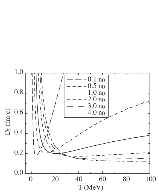
Figure 1: Isospin diffusion coefficient $D_{I}$ in symmetric matter, for $U_{i}=0$, at different indicated densities, as a function of the temperature $T$. In the high-temperature limit, the diffusion coefficient exhibits the behavior $D_{I}\propto\sqrt{T}/n$. Correspondingly, at high temperatures in the figure, the largest coefficient values are obtained for the lowest densities and the lowest coefficient values are obtained for the highest densities. In the low-temperature limit, the diffusion coefficient exhibits the behavior $D_{I}\propto n^{3/2}/T^{2}$ and the order of the results in density reverses.

The diffusivity for the experimental cross sections and no interaction contributions to the symmetry energy is shown at $\delta=0$ and different densities $n$ in Fig. 1, as a function of temperature $T$. At low temperatures, the diffusivity diverges due to a suppression of collisions by the Pauli principle. At high temperatures, compared to the Fermi energy, the role of the Pauli principle is diminished and the diffusivity acquires a characteristic $\sqrt{T}$ dependence. At moderate temperatures and densities in the vicinity and above normal, the diffusion coefficient turns out to be in the vicinity of our original estimate of $D_{I}\sim 0.2$ fm$\,c$.

It should be mentioned that, for symmetric matter, the factors for temperature and pressure gradients in the thermodynamic force ${\bf d}_{12}$ (28) vanish, $\Pi^{P}=0$ and $\Pi^{T}=0$, and the brace product in (40) vanishes, $\{{\bf A},{\bf C}\}=0$, yielding $k_{T}=0$ in (38). As physically required, the temperature and pressure gradients produce no relative motion of neutrons and protons for the symmetric matter.

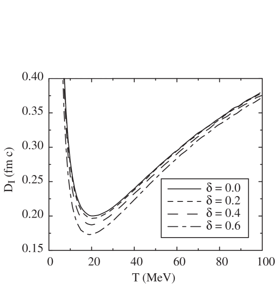
Figure 2: Isospin diffusion coefficient $D_{I}$ at normal density $n=n_{0}=0.16\,\mbox{fm}^{-3}$ and different indicated asymmetries $\delta$, for $U_{i}=0$, as a function of the temperature $T$. An increase in the asymmetry generally causes a decrease in the coefficient, as discussed in the text.

The diffusivity at normal density at different asymmetries is next shown in Fig. 2 as a function of temperature. Because of charge symmetry, the diffusivity does not depend on the sign of $\delta$. At low temperatures the diffusivity is generally expected to behave as

$$D_{I}\propto\frac{\hbar^{3}\,p_{F}^{2}}{m^{3}\,T^{2}\,\sigma}\,,$$ (68)

while at high temperatures in the manner prescribed by (53). With the respective behaviors serving as a guidance, we provide a parametrization of our numerical results for $D_{\delta}$ as a function of $n$, $T$ and $\delta$,

$$D_{I} = (1-0.19\,\delta^{2})\,\Bigg{[}\frac{11.34}{T^{2.38}}\,\left(\frac{n}{n_{0}}\right)^{1.54}$$ (69)

$$+\frac{1.746}{T}\,\left(\frac{n}{n_{0}}\right)^{0.56}+0.00585\,T^{0.913}\,\bigg{(}\frac{n_{0}}{n}\bigg{)}\Bigg{]}\,.$$

Here, the temperature $T$ is in MeV and the diffusivity $D_{I}$ is in fm$\,c$. The parametrization describes the numerical results to an accuracy better than 4% within the region of thermodynamic parameters of $1.0\leq n/n_{0}\leq 4.0$, $10\,\mbox{MeV}\leq T\leq 100\,\mbox{MeV}$ and $|\delta|\leq 0.4$. This is, generally, the parameter region of interest in intermediate-energy reactions.

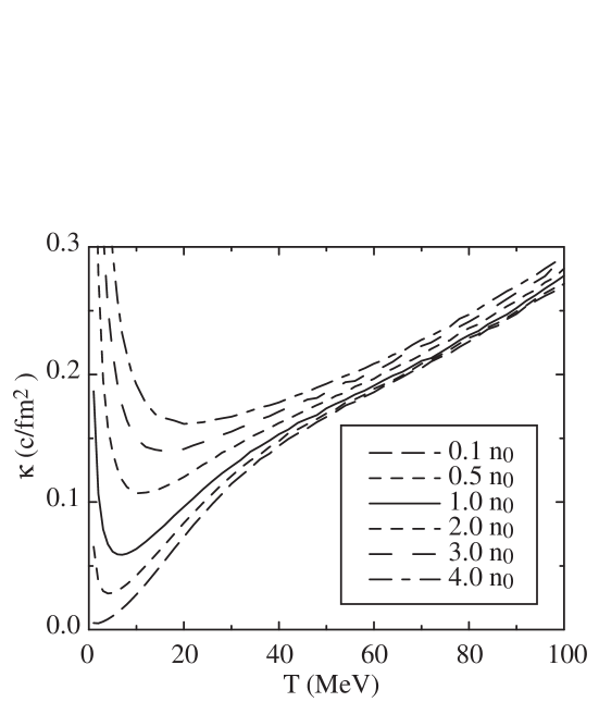
Figure 3: Thermal conductivity $\kappa$ in symmetric nuclear matter, at different indicated densities in units of $n_{0}$, as a function of temperature $T$. The conductivity increases as density increases.

The heat conductivity is shown for symmetric matter at different densities in Fig. 3, as a function of temperature. The results are similar to those in Ref. PD84 , though there the two component nature of nuclear matter was ignored and the isospin-averaged nucleon-nucleon cross-sections have been used. A closer examination of results in Subsections IV.3 and IV.4 indicates that the use of the isospin-averaged cross-sections is, actually, justified for symmetric matter, when calculating the heat-conduction and shear-viscosity coefficients. Otherwise, however, Fig. 3 has been based on a more complete set of cross sections than results in PD84 . As in the case of diffusivity, the heat conductivity diverges at low temperatures and tends to a classical behavior at high temperatures, exhibiting there no density dependence and being proportional to velocity, $\kappa\propto\sqrt{T}$. As in the case of diffusivity, we next provide a parametrization of our numerical results for the heat conductivity $\kappa$ as a function of $n$, $T$ and $\delta$,

$$\kappa = (1+0.10\,\delta^{2})\,\Bigg{[}\frac{0.235}{T^{0.755}}\,\bigg{(}\frac{n}{n_{0}}\bigg{)}^{0.951}$$ (70)

$$-0.0582\left(\frac{n}{n_{0}}\right)^{0.0816}+0.0238T^{0.5627}\,\left(\frac{n}{n_{0}}\right)^{0.0171}\Bigg{]}\,.$$

Here, $T$ is again in MeV and $\kappa$ is in c/fm². The parameterization agrees with the numerical results to an accuracy better than 4% within the range of thermodynamic parameters indicated in the case of $D_{I}$.

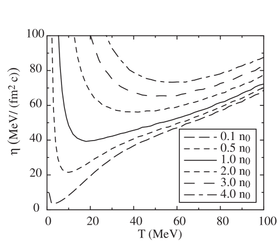
Figure 4: Shear viscosity $\eta$ in symmetric nuclear matter, at different indicated densities in units of $n_{0}$, as a function of temperature $T$. The viscosity increases as density increases.

The shear viscosity coefficient $\eta$ is shown for symmetric matter at at different densities, as a function of temperature, in Fig.4. Again, the results are similar to those in Ref. PD84 . At high temperatures, the dependence on density weakens and the viscosity becomes proportional to velocity. The numerical results for $\eta$ are well described, to an accuracy better than 4% within the before-mentioned range, by

$$\eta=(1+0.10\,\delta^{2})\,\Bigg{[}\frac{856}{T^{1.10}}\,\bigg{(}\frac{n}{n_{0}}\bigg{)}^{1.81}-\frac{240.9}{T^{0.95}}\left(\frac{n}{n_{0}}\right)^{2.12}+2.154\,T^{0.76}\Bigg{]}\,.$$ (71)

Here, $\eta$ is in MeV/fm${}^{2}\,c$ and $T$ is in MeV.

We note in (69)-(71), that the diffusion coefficient weakly drops with increasing magnitude of asymmetry $|\delta|$, while the viscosity and heat conduction coefficients weakly increase. Given the weaknesses of the dependencies, the behaviors exhibited in parametrizations represent, in practice, averages over the considered independent-parameter regions. Overall, the drop and rise in the respective coefficients with $|\delta|$ is characteristic for a situation where the local flux of a component grows faster than the concentration of that component. That type of growth, with the magnitude of asymmetry, typifies a mixture of degenerate fermion gases. The general trends can be deduced following the mean-free-path arguments from Sec. II. When the average velocity rises with asymmetry, so do the heat conduction and shear viscosity coefficients. Additional rise for those coefficients, in the case at hand, can result from the Pauli principle effects and from the difference between cross sections for like and unlike particles. Regarding the diffusion coefficient, though, one needs to consider an irreversible part of relative particle flux, under the condition of the concentration varying with position. If, starting with a given configuration of concentration gradients, one introduces uniform changes of concentration on top, not just the overall relative flux undergoes change but also the reversible flux of concentration gets altered. The rise in the relative flux associated with the velocity of a dominant component rising with concentration is normally more than compensated by the rise in reversible flux, leading to a reduction in the irreversible flux and producing a reduction in diffusivity with particle asymmetry. A mean-field example where the reversible flux eats into the net flux reducing the diffusivity with increasing asymmetry is the estimate in Eq. (10), obtained there without invoking the particle Fermi statistics.

As is found in Secs. III.3 and IV.2, the dependence of mean fields on species enters the diffusivity through the factor $\Pi^{\delta}$ resulting from the variable change in thermodynamic driving force, from the difference of chemical potentials per mass to asymmetry. The simplest case where one can consider the impact of the mean fields is that of the symmetric nuclear matter, at $\delta=0$. In this case, the factor may be represented as

$$\Pi^{\delta}=\frac{1}{m}\,\left(\frac{n}{\xi}+4a_{I}^{v}\right)\,,$$ (72)

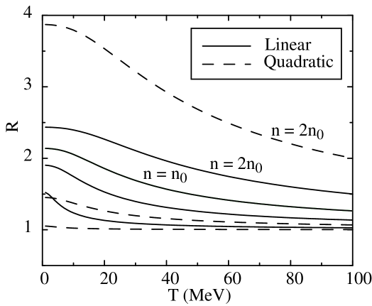
Figure 5: Mean-field enhancement factor of the diffusion coefficient in symmetric nuclear matter, $R\equiv D_{I}(U_{i})/D_{I}(U_{i}=0)$, at a fixed density $n$, as a function of temperature $T$. The solid and dashed lines, respectively, represent the factors for the assumed linear and quadratic dependence of the interaction symmetry energy on density. The lines from top to bottom are for densities $n=2\,n_{0}$, $n_{0}$, $0.5\,n_{0}$ and $0.1\,n_{0}$, respectively. At normal density the results for the two dependencies coincide.

where $\xi_{i}=\frac{\partial n_{i}}{\partial\mu_{i}}\equiv\xi$ (cf. Appendix C). At high temperatures, we have approximately $\xi_{i}\approx\frac{n_{i}}{T}$, so that $\frac{n}{\xi}\approx 2T$. The naive expectation is that $a_{I}^{v}$ has a linear dependence on the net density, $a_{I}^{v}=a_{I}^{v0}\left(\frac{n}{n_{0}}\right)^{\nu}$, where $a_{I}^{v0}=14$ MeV and $\nu=1$. The mean-field amplification factor $R=\Pi^{\delta}(a_{I}^{v})/\Pi^{\delta}(a_{i}^{v}=0)$ for the diffusion coefficient, assuming the linear and also quadratic density-dependence of $a_{I}^{v}$ ($\nu=1$ and 2) is shown in Fig. 5. The quadratic dependence gives higher amplification factors at $n>n_{0}$, than the linear dependence, while the opposite is true at $n<n_{0}$. At low temperatures and moderate to high densities the amplification is very strong suggesting that the diffusion could be used to probe the symmetry energy, aside from the in-medium neutron-proton cross sections.

V.2 Testing the Form-Factor Expansion

The calculations of transport coefficients above have been done assuming that the functions $a_{i}$, $b_{i}$ and $c_{i}$ in Eqs. (34) can be approximated by constants. In the more general case, the functions can be expanded in the series in $p^{2}$, e.g.

$$c_{i}(p^{2})=c_{i}^{(1)}+c_{i}^{(2)}\,p^{2}+c_{i}^{(3)}\,p^{4}+\ldots\,.$$ (73)

The coefficients of the expansion can be found by considering moments of the form-factor equations (31)-(33). With the more general form of the form-factor functions, the transport coefficients generally increase, but their rise is generally very limited.

To illustrate the magnitude of higher-order effects, we provide in Table 1 results for the diffusivity obtained in the standard first-order and in the higher-order calculations at sample densities and temperatures. In the indicated cases, the second-order calculations never increase the diffusion coefficient by more than 3% above the first-order calculations. The efficiency of our Monte-Carlo procedure employed to evaluate the integrals for coefficients worsens as the order of our calculations increases and, correspondingly, we provide only a single third-order result for illustration.

V.3 Isospin Equilibration

To test sensibility of the results on diffusivity and to gain an elementary insight into the process of isospin equilibration in a reaction, we carry out a schematic consideration of the equilibration. For definiteness, and to ensure a level of applicability for our consideration, we take the case of a ⁹⁶Ra + ⁹⁶Zr reaction at $E_{lab}/A=100\,\mbox{MeV}$. Densities in the central region of the reaction are not far from normal. Following the degenerate Fermi-gas limit, the temperature in the central region can be estimated with $T\sim\sqrt{E_{lab}/(2a)}\sim 20\,\mbox{MeV}$ using $a\approx A/(8\,\mbox{MeV})$; deviations from the degenerate limit yield a bit higher value. Under those conditions, basing on Figs. 1 and 5, we estimate the streaming contribution to the diffusivity in the central region at $0.21\,\mbox{fm}\,c$ and the mean-field contribution at $0.20\,\mbox{fm}\,c$, for a net $D_{I}\approx 0.41\,\mbox{fm}\,c$.

Considering the direction perpendicular to the plane of contact between the nuclei, with nuclei extending a distance $L\sim(A/n_{0})^{1/3}\sim 8\,\mbox{fm}$ both ways from the interface, we may use the one-dimensional diffusion equation to estimate the isospin equilibration

$$\frac{\partial\delta}{\partial t}=D_{I}\,\frac{\partial^{2}\delta}{\partial x^{2}}\,,$$ (74)

where $x$ is the direction perpendicular to the interface, cf. Eq. (7). With isospin flux vanishing at the boundaries of the region $[-L,L]$, the solution to (74) is

$$\delta(x,t)=\delta_{\infty}+\sum_{n=1}^{\infty}a_{n}\,\sin{k_{n}\,x}\,\exp{(-D_{I}\,k_{n}^{2}\,t)}+\sum_{n=1}^{\infty}b_{n}\,\cos{q_{n}\,x}\,\exp{(-D_{I}\,q_{n}^{2}\,t)}\,$$ (75)

where $k_{n}\,L=\left(n-\frac{1}{2}\right)\,\pi$ and $q_{n}\,L=n\,\pi$. The coefficients $a_{n}$ and $b_{n}$ are determined by the initial conditions and, in the case in question, $b_{n}=0$.

The different terms in the expansion (75) correspond to the different levels of detail in the distribution of concentration, as characterized by the different wavevectors. We see that the greater the detail the faster the information is erased, with the erasure rates proportional to wavevectors squared. The overall distribution tends towards $\delta_{\infty}$ as $t\rightarrow\infty$. The late-stage approach to equilibrium is governed by the rate for the term with the lowest wavevector, i.e. $a_{1}$. Defining the isospin equilibration time $t_{H}$ as one for which the original isospin asymmetry between the nuclei is reduced by half, we get from (75) an estimate for the reaction

$$t_{H}\approx\frac{\ln{2}}{D_{I}\,k_{1}^{2}}=\frac{4\ln{2}\,L^{2}}{\pi^{2}\,D_{I}}\sim 44\,\mbox{fm}/c\,,$$ (76)

for the case above. When we carry out the full respective Boltzmann-equation simulations of the $100\,\mbox{MeV/nucleon}$ ⁹⁶Ru + ⁹⁶Zr reactions, at the impact parameter of $b=5\,\mbox{fm}\gtrsim L/2$ (to ensure a neck comparable to that in the consideration), we find that, indeed, the nuclei need to be in contact for about $40\,\mbox{fm}/c$ for the isospin asymmetry to drop to the half of original value.

VI Summary

Diffusion and other irreversible transport phenomena have been discussed for a binary Fermi system close to equilibrium. For weak nonuniformities, the irreversible fluxes are linear in the uniformities, with the characteristic transport proportionality-coefficients dependent only on the equilibrium system. It is hoped that, in an analogy to how the nuclear equation of state and symmetry energy are employed, the coefficient of diffusion can be employed to characterize reacting nuclear systems with respect to isospin transport.

Following a qualitative discussion of the irreversible transport in the paper, the set of coupled Boltzmann-Uhlenbeck-Uehling equations was considered for a binary system, assuming slow macroscopic temporal and spatial changes. The slow changes allow to solve the equation set by iteration, with the lowest-order solution being the local equilibrium distributions. In the next order, corrections to those distributions were obtained, linear in the thermodynamic driving forces associated with the system nonuniformities. These corrections produce irreversible fluxes linear in the forces. The transport coefficients have been formally expressed in terms of brace products of the responses of distribution functions to the driving forces. The considered coefficients include diffusivity, conductivity, heat conduction and shear viscosity.

The set of the linearized Boltzmann equations was, further, explicitly solved under the assumption of simplified distribution-function responses to the thermodynamic driving forces. The solutions to the equations led to explicit expressions for the transport coefficients, with the diffusivity given in terms of the collision integral for collisions between the two species weighted by the momentum transfer squared. Besides associated sensitivity to the cross section for collisions between the species, the diffusivity is also sensitive to the dependence of mean fields on the species. The collisions between the species are those that inhibit the relative motion of the species; the difference between mean fields affects the relative acceleration and, in combination with the collisions, the stationary diffusive flux that is established.

We calculated the isospin diffusivity for nuclear matter, using experimental nucleon-nucleon cross sections for species-independent mean-fields. At low temperatures and high densities, the diffusivity diverges due a suppression of collisions by the Pauli principle. At high temperatures, the diffusivity is roughly proportional to the average velocity and is inversely proportional to the density. The diffusivity weakly decreases with an increase in the absolute magnitude of asymmetry. We provided an analytic fit to our numerical results. For completeness, we also calculated the heat conduction and shear viscosity coefficients and provided fits to those. Moreover, we calculated the diffuseness mean-field enhancement factor for symmetric matter, assuming a couple of dependencies of the symmetry energy on density. At low temperatures, the enhancement factor is simply proportional to the net symmetry energy divided by the kinetic symmetry energy. Considering the expansion of the form-factors in distribution-function responses, we demonstrated that corrections to the Boltzmann-equation transport coefficients, beyond the approximations we employed, are small. Finally, we produced an elementary estimate for isospin equilibration in a low impact-parameter collision.

Appendix A Macroscopic Quantities

We shall consider different types of macroscopic quantities, either net or for separate components, either in the general frame of observation or in a local frame. For a single component $i$ in the observation frame, the density $n_{i}$, mean velocity $\underline{\bf v}_{i}$, mean kinetic energy $\underline{e_{i}}$, momentum flux tensor $\overline{\overline{p}}_{i}$ and kinetic energy flux ${\bf q}_{i}$, are given in terms of the distribution $f_{i}$, respectively, as

$$n_{i}({\bf r},t) = \frac{g}{(2\pi\hbar)^{3}}\int{d^{3}p}\,f_{i}({\bf p},{\bf r},t)\,,$$ (77a)

$$n_{i}\,\underline{\bf v}_{i} = \frac{g}{(2\pi\hbar)^{3}}\int{d^{3}p}\,\frac{\bf p}{m_{i}}\,f_{i}({\bf p},{\bf r},t)\,,$$ (77b)

$$n_{i}\,\underline{e}_{i} = \frac{g}{(2\pi\hbar)^{3}}\int{d^{3}p}\,\frac{p^{2}}{2m_{i}}\,f_{i}({\bf p},{\bf r},t)\,,$$ (77c)

$$\overline{\overline{p}}_{i} = \frac{g}{(2\pi\hbar)^{3}}\int{d^{3}p}\,\frac{\overline{\overline{{\bf p\,p}}}}{m_{i}}\,f_{i}({\bf p},{\bf r},t)\,,$$ (77d)

$${\bf q}_{i} = \frac{g}{(2\pi\hbar)^{3}}\int{d^{3}p}\,\frac{p^{2}}{2m_{i}}\,\frac{{\bf p}}{m_{i}}\,f_{i}({\bf p},{\bf r},t)\,.$$ (77e)

The net quantities result from combining the component contributions. Thus, the net density is $n=n_{1}+n_{2}$, the net mass density is $\rho=\rho_{1}+\rho_{2}=m_{1}\,n_{1}+m_{2}\,n_{2}$ while the net velocity $\underline{\bf v}$ is obtained from $\rho\,\underline{\bf v}=\rho_{1}\,\underline{\bf v}_{1}+\rho_{2}\,\underline{\bf v}_{2}$. The kinetic energy $\underline{e}$ averaged over all particles is given by $n\,\underline{e}=n_{1}\,\underline{e}_{1}+n_{2}\,\underline{e}_{2}$, the net momentum flux is $\overline{\overline{p}}=\overline{\overline{p}}_{1}+\overline{\overline{p}}_{2}$ and the net kinetic energy flux is ${\bf q}={\bf q}_{1}+{\bf q}_{2}$.

Local quantities are those calculated with momenta transformed to the local mass frame, i.e. following the substitution ${\bf p}\rightarrow{\bf p}-m_{i}\,\underline{\bf v}$. To distinguish local quantities from those in the observation frame, when the frame matters, the local quantities will be capitalized. The local momentum flux tensor $\overline{\overline{P}}$ is the kinetic pressure tensor and the local kinetic energy flux ${\bf Q}$ is the heat flux.

Appendix B continuity equations

The collisions in the Boltzmann equation set (13) conserve the quasiparticle momentum and energy and the species identity. This leads to local conservation laws for the corresponding macroscopic quantities.

Let $\chi_{j}({\bf p})$ represent one of the quasiparticle quantities conserved in collisions, $\chi_{j}({\bf p})=\delta_{ij}$, ${\bf p}$ or $p^{2}/2m_{j}$. For those quantities, the integration with collision integrals produces

$$\sum_{j}\int d^{3}p\,\chi_{j}\,J_{j}=0\,.$$ (78)

As a consequence, from the Boltzmann equation set, we obtain

$$\sum_{j}\int\frac{d^{3}p}{(2\pi\hbar)^{3}}\,\chi_{j}\,\left({\frac{\partial f_{j}}{\partial t}}+\frac{\bf p}{m_{j}}\cdot\frac{\partial{f_{j}}}{\partial{\bf r}}+{\bf F}_{j}\cdot\frac{\partial{f_{j}}}{\partial{\bf p}}\right)=0\,.$$ (79)

After a partial integration, we get from the above

$$\frac{\partial}{\partial t}\left(n\underline{\chi}\right)+\frac{\partial}{\partial{\bf r}}\cdot\left(n\,\underline{\frac{\bf p}{m}\,\chi}\right)-n\,\underline{{\bf F}\cdot\frac{\partial\chi}{\partial{\bf p}}}=0\,,$$ (80)

where the averages are defined with

$$n\,\underline{\chi}=\sum_{j}\int\frac{d^{3}p}{(2\pi\hbar)^{3}}\,\chi_{j}\,f_{j}({\bf p},{\bf r},t)\,.$$ (81)

Substituting for $\chi_{j}$ the conserved quantities ($\chi_{j}({\bf p})=\delta_{ij}$, ${\bf p}$ or $p^{2}/2m_{j}$), we get the respective continuity equations:

$$\frac{\partial n_{i}}{\partial t}+\frac{\partial}{\partial{\bf r}}\cdot\left(n_{i}\,\underline{\bf v}_{i}\right)=0\,$$ (82a)

$$\frac{\partial}{\partial t}\left(\rho\,\underline{\bf v}\right)+\frac{\partial}{\partial{\bf r}}\cdot\overline{\overline{p}}-n_{1}\,{\bf F}_{1}-n_{2}\,{\bf F}_{2}=0\,,$$ (82b)

$$\frac{\partial}{\partial t}\left(n\,\underline{e}\right)+\frac{\partial}{\partial{\bf r}}\cdot{\bf q}-n_{1}\,\underline{\bf v}_{1}\cdot{\bf F}_{1}-n_{2}\,\underline{\bf v}_{2}\cdot{\bf F}_{2}=0\,.$$ (82c)

Here, we made yet no use of the local frame.

The local frame is useful when wants to make use of the assumption of local equilibrium that imposes restrictions on local quantities. On representing the average velocities as $\underline{\bf v}_{i}=\underline{\bf V}_{i}+\underline{\bf v}$ in the equations above, we obtain the following set,

$$\frac{\partial n_{i}}{\partial t}+\frac{\partial}{\partial{\bf r}}\cdot\left(n_{i}\,\underline{\bf v}\right)+\frac{\partial}{\partial{\bf r}}\cdot\left(n_{i}\,\underline{\bf V}_{i}\right)=0\,,$$ (83a)

$$\frac{\partial\rho}{\partial t}+\frac{\partial}{\partial{\bf r}}\cdot\left(\rho\,\underline{\bf v}\right)=0\,,$$ (83b)

$$\frac{\partial}{\partial t}\left(\rho{\bf v}\right)+\frac{\partial}{\partial{\bf r}}\cdot\left(\rho\,{\bf v\,v}\right)+\frac{\partial}{\partial{\bf r}}\cdot\overline{\overline{P}}-n_{1}\,{\bf F}_{1}-n_{2}\,{\bf F}_{2}=0\,,$$ (83c)

$$\frac{\partial}{\partial t}\left(n\,\underline{E}\right)+\frac{\partial}{\partial{\bf r}}\cdot\left(n\,\underline{E}\,{\bf v}\right)+\overline{\overline{P}}:\overline{\overline{\frac{\partial}{\partial{\bf r}}\,{\bf v}}}+\frac{\partial}{\partial{\bf r}}\cdot{\bf Q}-n_{1}\,\underline{\bf V}_{1}\,{\bf F}_{1}-n_{2}\,\underline{\bf V}_{2}\,{\bf F}_{2}=0\,.$$ (83d)

The equation for mass density in the set above follows from combining the equations for particle densities.

The above equations significantly simplify when the assumption of a strict local equilibrium is imposed. Under that assumption, the local species velocities and the heat flow vanish, ${\bf V}_{i}=0$ and ${\bf Q}=0$, and the kinetic pressure tensor becomes diagonal, $\overline{\overline{P}}=\frac{2}{3}\,n\,\underline{E}\,\overline{\overline{1}}$. The equations reduce then to the Euler set

$$\frac{\partial n_{i}}{\partial t}+\frac{\partial}{\partial{\bf r}}\cdot\left(n_{i}\,\underline{\bf v}\right)=0\,,$$ (84a)

$$\frac{\partial}{\partial t}\left(\rho{\bf v}\right)+\frac{\partial}{\partial{\bf r}}\cdot\left(\rho\,\overline{\overline{\bf v\,v}}\right)+\frac{2}{3}\,\frac{\partial(n\,\underline{E})}{\partial{\bf r}}-n_{1}\,{\bf F}_{1}-n_{2}\,{\bf F}_{2}=0\,,$$ (84b)

$$\frac{\partial}{\partial t}\left(n\,\underline{E}\right)+{\bf v}\cdot\frac{\partial}{\partial{\bf r}}\left(n\,\underline{E}\right)+\frac{5}{3}\,n\,\underline{E}\,\frac{\partial}{\partial{\bf r}}\cdot{\bf v}=0\,.$$ (84c)

Appendix C Space-Time Derivatives for an Ideal Fluid

In an ideal fluid, all local quantities can be expressed in terms of the local temperature $T$ and the local kinetic chemical potential $\mu_{i}$. If we consider changes of the densities $n_{i}$ or of the local kinetic energies $\underline{E}_{i}$ with respect to a parameter $x$ representing some spatial coordinate or time, or their combination, we find

$$\frac{\partial n_{i}}{\partial x} = \xi_{i}\,T\,\frac{\partial\alpha_{i}}{\partial x}+\frac{3}{2}\,n_{i}\,\frac{\partial\beta}{\partial x}\,,$$

$$\frac{\partial(n_{i}\,\underline{E}_{i})}{\partial x} = \frac{3}{2}\,n_{i}\,T\frac{\partial\alpha_{i}}{\partial x}+\frac{5}{2}\,n_{i}\,\underline{E}_{i}\,\frac{\partial\beta}{\partial x}\,,$$ (85)

where $\alpha_{i}=\mu_{i}/T$, $\beta=\log{T}$ and $\xi_{i}=(\partial n_{i}/\partial\mu_{i})_{T}$. With the trace derivative defined as

$$\frac{d}{dt}=\frac{\partial}{\partial t}+{\bf v}\cdot\frac{\partial}{\partial{\bf r}}\,,$$

a particular version of the above relations is

$$\frac{dn_{i}}{dt} = \xi_{i}\,T\,\frac{d\alpha_{i}}{dt}+\frac{3}{2}\,n_{i}\,\frac{d\beta}{dt}\,,$$

$$\frac{d(n_{i}\,\underline{E}_{i})}{dt} = \frac{3}{2}\,n_{i}\,T\frac{d\alpha_{i}}{dt}+\frac{5}{2}\,n_{i}\,\underline{E}_{i}\,\frac{d\beta}{dt}\,.$$ (86)

A combination of the above trace-derivative relations with the Euler equations from Appendix B yields the following simple results,

$$\frac{d\alpha_{i}}{dt} = 0\,,$$ (87a)

$$\frac{d\beta}{dt} = -\frac{2}{3}\,\frac{\partial}{\partial{\bf r}}\cdot{\bf v}\,,$$ (87b)

the consistency of which with (86) and (84) is easy to verify. The results (87) express basic features of the isentropic ideal-fluid evolution of a mixture. The entropy per particle in species $i$ depends only on $\alpha_{i}$, while the ratio of the densities of species $n_{1}/n_{2}$ depends both on $\alpha_{1}$ and $\alpha_{2}$. The conservation of $\alpha_{i}$ for both species is equivalent to the conservation of entropy per particle and of relative concentration. Finally, the density for species $i$ is proportional to $T^{3/2}$ multiplying a function of $\alpha_{i}$, which is equivalent to the second of the results above, given the continuity equation for species and the conservation of $\alpha_{i}$.

Appendix D Variable Transformation

The driving forces for diffusion are naturally expressed in terms of the gradients of temperature and of chemical potential difference per unit mass $\mu_{12}^{t}$. However, given the typical constraints on systems, it can be convenient to express the chemical potential in terms of other quantities, that are easier to assess or control, such as the differential concentration $\delta$, temperature $T$ and net pressure $P^{t}$. A transformation of the variables for the driving forces has been employed, at a formal level, in Sec. III.3. Here, we show, though, how the transformation can be done in practice for the interaction energy per particle specified in terms of the particle density $n$ and concentration $\delta$, $E^{v}=E^{v}(n,\delta)$. With the nuclear application in mind, we limit ourselves to the case of $m_{1}=m_{2}=m$.

The transformation can exploit straightforward relations between different differentials. One of those to exploit is the Gibbs-Duhem relation

$$dP^{t}=n_{1}\,d\mu_{1}^{t}+n_{2}\,d\mu_{2}^{t}+n\,s\,dT=n\,d\mu^{t}+\frac{m\,n\,\delta}{2}\,d\mu_{12}^{t}+n\,s\,dT\,.$$ (88)

Here, $s$ is the entropy per particle and $\mu^{t}=(\mu_{1}^{t}+\mu_{2}^{t})/2$ is the median chemical potential. Two other relations stem from the differentiations of equilibrium particle distributions, already utilized in Appendix C,

$$dn_{i}=\xi_{i}\,d\mu_{i}+\frac{\frac{3}{2}n_{i}-\xi_{i}\,\mu_{i}}{T}\,dT\equiv\xi_{i}\,d\mu_{i}+\left(\frac{\partial n_{i}}{\partial T}\right)_{\mu_{i}}\,dT\,.$$ (89)

With $\mu_{i}^{v}={\partial(n\,E^{v})}/{\partial n_{i}}$, on adding and subtracting the two ($i=1,2$) relations side by side, we find

$$dn = \left(\xi_{1}+\xi_{2}\right)\left[d\mu^{t}-\left(\frac{\partial\mu^{v}}{\partial n}\right)_{\delta}\,dn-\left(\frac{\partial\mu^{v}}{\partial\delta}\right)_{n}\,d\delta\right]+\frac{m}{2}\left(\xi_{1}-\xi_{2}\right)$$ (90)

$$\times\left[d\mu_{12}^{t}-\left(\frac{\partial\mu_{12}^{v}}{\partial n}\right)_{\delta}\,dn-\left(\frac{\partial\mu_{12}^{v}}{\partial\delta}\right)_{n}\,d\delta\right]+\left[\left(\frac{\partial n_{1}}{\partial T}\right)_{\mu_{1}}+\left(\frac{\partial n_{2}}{\partial T}\right)_{\mu_{2}}\right]\,dT\,$$

and

$$\delta\,dn + n\,d\delta=\left(\xi_{1}-\xi_{2}\right)\left[d\mu^{t}-\left(\frac{\partial\mu^{v}}{\partial n}\right)_{\delta}\,dn-\left(\frac{\partial\mu^{v}}{\partial\delta}\right)_{n}\,d\delta\right]+\frac{m}{2}\left(\xi_{1}+\xi_{2}\right)$$ (91)

$$\times\left[d\mu_{12}^{t}-\left(\frac{\partial\mu_{12}^{v}}{\partial n}\right)_{\delta}\,dn-\left(\frac{\partial\mu_{12}^{v}}{\partial\delta}\right)_{n}\,d\delta\right]+\left[\left(\frac{\partial n_{1}}{\partial T}\right)_{\mu_{1}}-\left(\frac{\partial n_{2}}{\partial T}\right)_{\mu_{2}}\right]\,dT\,.$$

Those two equations have the structure

$$G_{kn}\,dn=G_{k\mu}\,d\mu^{t}+G_{kd}\,d\mu_{12}^{t}+G_{k\delta}\,d\delta+G_{kT}\,dT\,,$$ (92)

where $k=1,2$ and where the coefficients $G$ can be worked out from (90) and (91). On multiplying the sides of the first ($k=1$) equation by $G_{2n}$ and the sides of the second ($k=2$) equation by $G_{1n}$ and on subtracting the equations side by side, we can eliminate the $dn$ differential obtaining

$$0 = (G_{2n}\,G_{1\mu}-G_{1n}\,G_{2\mu})\,d\mu^{t}+(G_{2n}\,G_{1d}-G_{1n}\,G_{2d})\,d\mu_{12}^{t}$$ (93)

$$+(G_{2n}\,G_{1\delta}-G_{1n}\,G_{2\delta})\,d\delta+(G_{2n}\,G_{1T}-G_{1n}\,G_{2T})\,dT$$

$$\equiv R_{\mu}\,d\mu^{t}+R_{d}\,d\mu_{12}^{t}+R_{\delta}\,d\delta+R_{T}\,dT\,.$$

On eliminating next the $d\mu_{t}$ differential using the Gibbs-Duhem relation, we find

$$\Pi_{12}^{P} = \left(\frac{\partial\mu_{12}^{t}}{\partial P^{t}}\right)_{T,\delta}=\frac{R_{\mu}}{n\,\left(R_{\mu}\,\frac{m\,\delta}{2}-R_{d}\right)}\,,$$ (94a)

$$\Pi_{12}^{T} = \left(\frac{\partial\mu_{12}^{t}}{\partial T}\right)_{P^{t},\delta}=\frac{R_{\mu}\,s-R_{T}}{R_{d}-R_{\mu}\,\frac{m\,\delta}{2}}\,,$$ (94b)

$$\Pi_{12}^{\delta} = \left(\frac{\partial\mu_{12}^{t}}{\partial\delta}\right)_{P^{t},T}=\frac{R_{\delta}}{R_{\mu}\,\frac{m\,\delta}{2}-R_{d}}\,.$$ (94c)

Appendix E Brace Algebra

The brace products are employed in finding the transport coefficients within linear approximation to the Boltzmann equation. The brace product of two scalar quantities $A$ and $B$ associated with the colliding particles is defined as

$$\{A,B\} = \int\frac{d^{3}p}{(2\pi)^{3}}\,A_{1}\,I_{11}(B)+\int\frac{d^{3}p}{(2\pi)^{3}}\,A_{1}\,I_{12}(B)$$ (95)

$$+\int\frac{d^{3}p}{(2\pi)^{3}}\,A_{2}\,I_{21}(B)+\int\frac{d^{3}p}{(2\pi)^{3}}\,A_{2}\,I_{22}(B)$$

$$= \left[A,B\right]_{11}+\left[A,B\right]_{12}+\left[A,B\right]_{22}\,,$$

where, in the last step, we have broken the brace product into square-bracket products representing contributions from collisions within species $1$, from collisions between species $1$ and $2$ and from collisions within species $2$, respectively.

We will first show that the square-bracket product is symmetric. Thus, we have explicitly

$$\left[A,B\right]_{ii} = \frac{1}{2}\int\frac{d^{3}p_{a}}{(2\pi)^{3}}\,\frac{d^{3}p_{b}}{(2\pi)^{3}}\,d\Omega\,v^{*}\,\left(\frac{d\sigma_{ii}}{d\Omega}\right)\,f_{ia}^{(0)}\,f_{ib}^{(0)}\,{\tilde{f}_{ia}^{(0)\prime}}\,{\tilde{f}_{ib}^{(0)\prime}}\,$$ (96)

$$\times A_{ia}\,(B_{ia}+B_{ib}-B_{ia}^{\prime}-B_{ib}^{\prime})$$

$$= \frac{1}{8}\int\frac{d^{3}p_{a}}{(2\pi)^{3}}\,\frac{d^{3}p_{b}}{(2\pi)^{3}}\,d\Omega\,v^{*}\,\left(\frac{d\sigma_{ii}}{d\Omega}\right)\,f_{ia}^{(0)}\,f_{ib}^{(0)}\,{\tilde{f}_{ia}^{(0)\prime}}\,{\tilde{f}_{ib}^{(0)\prime}}\,$$

$$\times(A_{ia}+A_{ib}-A_{ia}^{\prime}-A_{ib}^{\prime})\,(B_{ia}+B_{ib}-B_{ia}^{\prime}-B_{ib}^{\prime})\,,$$

where, to get the last result, we have first utilized an interchange of the particles in the initial state of a collision and then an interchange of the initial and final states within a collision. It is apparent that the r.h.s. of (96) is symmetric under the interchange of $A$ and $B$. Moreover, we can see that a square bracket for $B=A$, $[A,A]_{ii}$, is nonnegative and that it vanishes only when $A$ is conserved in collisions.

We next consider the contribution from collisions between different species,

$$\left[A,B\right]_{12} = \int\frac{d^{3}p_{1}}{(2\pi)^{3}}\,\frac{d^{3}p_{2}}{(2\pi)^{3}}\,d\Omega\,v^{*}\,\left(\frac{d\sigma_{12}}{d\Omega}\right)\,f_{1}^{(0)}\,f_{2}^{(0)}\,{\tilde{f}_{1}^{(0)\prime}}\,{\tilde{f}_{2}^{(0)\prime}}\,$$ (97)

$$\times(A_{1}+A_{2})\,(B_{1}+B_{2}-B_{1}^{\prime}-B_{2}^{\prime})$$

$$= \frac{1}{2}\int\frac{d^{3}p_{1}}{(2\pi)^{3}}\,\frac{d^{3}p_{2}}{(2\pi)^{3}}\,d\Omega\,v^{*}\,\left(\frac{d\sigma_{12}}{d\Omega}\right)\,f_{1}^{(0)}\,f_{2}^{(0)}\,{\tilde{f}_{1}^{(0)\prime}}\,{\tilde{f}_{2}^{(0)\prime}}\,$$

$$\times(A_{1}+A_{2}-A_{1}^{\prime}-A_{2}^{\prime})\,(B_{1}+B_{2}-B_{1}^{\prime}-B_{2}^{\prime})\,.$$

Here, we again utilized an interchange between the initial and final states and we again observe a symmetry between $A$ and $B$ on the r.h.s. Thus, indeed, all square brackets are symmetric. Moreover, for $B=A$, we see that $[A,A]_{12}\geq 0$ and that the zero is only reached if $A$ is conserved.

Combining the results, we find that the brace product (95) is symmetric. Moreover, we find that the brace product of quantity $A$ with itself is nonnegative, $\{A,A\}\geq 0$, and vanishes only when $A$ is conserved. As the brace product has features of a pseudo-scalar product, a version of the Cauchy-Schwarz-Buniakowsky (CSB) inequality Gradshteyn holds,

$$\{A,A\}\,\{B,B\}\geq\left(\{A,B\}\right)^{2}\,.$$ (98)

All the results from this Appendix remain valid, in an obvious manner, when the brace product (95) is generalized to the pairs of tensors of the same rank associated with the particles, when requiring that the tensor indices are convoluted between the two tensors in the brace, as e.g. in (36). The positive definite nature of the brace product is important in ensuring that expressions for transport coefficients, obtained in the paper, yield positive values for the coefficients that in this case represent a stable system.

Table 1: Diffusion coefficient $D_{I}$ obtained within different orders of calculation, using experimental np cross sections, at sample densities $n$ and temperatures $T$ in symmetric nuclear matter, for species-independent mean fields. The numerical errors of the results on $D_{I}$ are indicated in parenthesis for the least-significant digits. The last two columns, separated by the ’$\pm$’ sign, give, respectively, the relative change in the result for the highest calculated order compared to the first order and the error for that change.

n	T		$D_{I}$		Relative
		$1^{\mbox{st}}$ order	$2^{\mbox{nd}}$ order	$3^{\mbox{rd}}$ order	Change
fm-3	MeV		fm$\,c$		$\%$
0.016	10	0.29949(15)	0.3055(12)		2.0	$\pm$	0.4
0.016	60	2.3891(18)	2.390(14)		0.0	$\pm$	0.6
0.16	10	0.27964(21)	0.2800(29)	0.2809(25)	0.5	$\pm$	0.9
0.16	60	0.29591(24)	0.2965(19)		0.2	$\pm$	0.7
0.32	10	0.4446(15)	0.4465(26)		0.4	$\pm$	0.7
0.32	60	0.18187(15)	0.1827(13)		0.5	$\pm$	0.7

References

- (1) J. M. Lattimer and M. Prakash, Astrophys. J. 550, 426 (2001).
- (2) F. Rami et al., Phys. Rev. Lett. 84, 1120 (2000).
- (3) G. F. Bertsch, S. Das Gupta, Phys. Rep. 160, 189 (1988).
- (4) J. Aichelin, Phys. Rep. 202, 233 (1991).
- (5) S. Tomonaga, Z. Phys. 110, 573 (1938).
- (6) V. M. Galitskii et al., Yad. Fiz. 30, 778 (1979) [Sov. J. Nucl. Phys. 30, 401 (1979).]
- (7) P. Danielewicz, Phys. Lett. 146 B, 168 (1984).
- (8) R. Hakim, L. Mornas, P. Peter, and H. D. Sivak, Phys. Rev. D 46, 4603 (1992).
- (9) R. Hakim and L. Mornas, Phys. Rev. C 47, 2846 (1993).
- (10) P. Danielewicz, Acta Phys. Polonica B 33, 45 (2002).
- (11) S. Chapman and T. G. Cowling, The Mathematical Theory of Non-Uniform Gases (Cambridge, New York, 1964).
- (12) E. A. Uehling and G. E. Uhlenbeck, Phys. Rev. 43, 552 (1933).
- (13) E. A. Uehling, Phys. Rev. 46, 917 (1934).
- (14) E. J. Hellund and E. A. Uehling, Phys. Rev. 56, 818 (1939).
- (15) R. L. Liboff, Kinetic Theory, Classical, Quantum, and Relativistic Descriptions (Prentice Hall, Englewood Cliffs, New Jersey, 1990).
- (16) L. D. Landau and E. M. Lifshitz, Fluid Mechanics, Vol. 6 of Course of Theoretical Physics (Addison-Wesley, Reading, 1959).
- (17) S. R. De Groot and P. Mazur, Non-Equilibrium Thermodynamics (North-Holland, Amsterdam, 1962).
- (18) G. Baym and C. Pethick, Landau Fermi-Liquid Theory (John Wiley & Sons, New York, 1991).
- (19) V. Greco, M. Colonna, M. Di Toro and F. Matera, Phys. Rev. C67, 015203(2003).
- (20) S. J. Yennello et al., Phys. Lett. B 321, 15 (1994); H. Johnston et al., Phys. Lett. B 371, 186 (1996); H. Johnston et al., Phys. Rev. C 56, 1972 (1997).
- (21) I. S. Gradshteyn and I. M. Ryzhik, Table of Integrals, Series, and Products (Academic Press, New York, 1979).