TWO-PION EXCHANGE
NUCLEON-NUCLEON POTENTIAL:
${\cal O}(q^{4})$ RELATIVISTIC CHIRAL EXPANSION

Abstract

We present a relativistic procedure for the chiral expansion of the two-pion exchange component of the $NN$ potential, which emphasizes the role of intermediate $\pi N$ subamplitudes. The relationship between power counting in $\pi N$ and $NN$ processes is discussed and results are expressed directly in terms of observable subthreshold coefficients. Interactions are determined by one- and two-loop diagrams, involving pions, nucleons, and other degrees of freedom, frozen into empirical subthreshold coefficients. The full evaluation of these diagrams produces amplitudes containing many different loop integrals. Their simplification by means of relations among these integrals leads to a set of intermediate results. Subsequent truncation to ${\cal O}(q^{4})$ yields the relativistic potential, which depends on six loop integrals, representing bubble, triangle, crossed box, and box diagrams. The bubble and triangle integrals are the same as in $\pi N$ scattering and we have shown that they also determine the chiral structures of box and crossed box integrals. Relativistic threshold effects make our results to be not equivalent with those of the heavy baryon approach. Performing a formal expansion of our results in inverse powers of the nucleon mass, even in regions where this expansion is not valid, we recover most of the standard heavy baryon results. The main differences are due to the Goldberger-Treiman discrepancy and terms of ${\cal O}(q^{3})$, possibly associated with the iteration of the one-pion exchange potential.

I introduction

A considerable refinement in the description of nuclear interactions has occurred in the last decade, due to the systematic use of chiral symmetry. As the non-Abelian character of QCD prevents low-energy calculations, one works with effective theories that mimic, as much as possible, the basic theory. In the case of nuclear processes, where interactions are dominated by the quarks $u$ and $d$, these theories are required to be Poincaré invariant and to have approximate $SU(2)\times SU(2)$ symmetry. The latter is broken by the small quark masses, which give rise to the pion mass at the effective level.

In the 1960s, it became well established that the one-pion exchange potential (OPEP) provides a good description of $NN$ interactions at large distances. When one moves inward, the next class of contributions corresponds to exchanges of two uncorrelated pions [1] and, until recently, there was no consensus in the literature as how to treat this component of the force. An important feature of the two-pion exchange potential (TPEP) is that it is closely related to the pion-nucleon ($\pi$N) amplitude, a point stressed more than thirty-five years ago by Cottingham and Vinh Mau [2]. This idea allowed one to overcome the early difficulties associated with perturbation theory [3] and led to the construction of the successful Paris potential [4], where the intermediate part of the interaction is obtained by means of dispersion relations. This has the advantages of minimizing the number of unnecessary hypotheses and yielding model independent results, but it does not help in clarifying the role of different dynamical processes, which are always treated in bulk.

Field theory provides an alternative framework for the evaluation of the TPEP. In this case, one uses a Lagrangian, involving the degrees of freedom one considers to be relevant, and calculates amplitudes using Feynman diagrams, which are subsequently transformed into a potential. An important contribution along this line was given in the early 1970s by Partovi and Lomon, who considered box and crossed box diagrams, using a Lagrangian containing just pions and nucleons with pseudoscalar (PS) coupling [5]. A study of the same diagrams using a pseudovector (PV) coupling was performed later by Zuilhof and Tjon [6]. The development of this line of research led to the Bonn model for the $NN$ interaction, which included many important degrees of freedom and proved to be effective in reproducing empirical data [7]. On the phenomenological side, accurate potentials also exist, which can reproduce low-energy observables employing parametrized forms of the two-pion exchange component [8].

Nowadays, it is widely acknowledged that chiral symmetry provides the best conceptual framework for the construction of nuclear potentials. The importance of this symmetry was pointed out in the 1970s by Brown and Durso [9] and by Chemtob, Durso, and Riska [10], who stressed that it constrains the form of the intermediate $\pi$N amplitude present in the TPEP.

In the early 1990s, the works by Weinberg restating the role of chiral symmetry in nuclear interactions [11] were followed by an effort by Ordóñez and van Kolck [12] and other authors [13, 14] to construct the TPEP in that framework. The symmetry was then realized by means of non linear Lagrangians containing only pions and nucleons. This minimal chiral TPEP is consistent with the requirements of chiral symmetry and reproduces, at the nuclear level, the well known cancellations present in the intermediate $\pi N$ amplitude [15]. On the other hand, a Lagrangian containing just pions and nucleons could not describe experimental $\pi N$ data [16] and the corresponding potential missed even the scalar-isoscalar medium range attraction [14].

One needed other degrees of freedom. The $\Delta$ contributions were shown to improve predictions by Ordóñez, Ray, and van Kolck [17] and other authors [18]. Empirical information about the low-energy $\pi N$ amplitude is normally summarized by means of subthreshold coefficients [16, 19], which can be used either directly in the construction of the TPEP or to determine unknown coupling constants (LECs) in chiral Lagrangians. The inclusion of this information allowed satisfactory descriptions of the asymptotic $NN$ data to be produced, with no need of free parameters [20, 21, 22, 23].

As far as techniques for implementing the symmetry are concerned, recent calculations of the TPEP were performed using both heavy baryon chiral perturbation theory (HBChPT) and covariant Lagrangians. In the former case [12, 17, 21, 22, 23, 24], one uses non relativistic effective Lagrangians, which include unknown counterterms, and amplitudes are derived in which loop and counterterm contributions are organized in well defined powers of a typical low-energy scale. In this approach, relativistic corrections required by precision have to be added separately [25].

QCD is a theory without formal ambiguities and the same should happen with effective theories designed to be used at the hadron level. In the case of nuclear interactions, this allows one to expect that the chiral TPEP should be unique, except for the iteration of the OPEP, which depends on the dynamical equation employed.

In the meson sector, chiral perturbation is indeed unique and predictions at a given order are unambiguous. However, the problem becomes much more difficult for systems containing baryons. At present, the uniqueness problem is under scrutiny and two competing calculation procedures are available based on either heavy baryon (HBChPT) or relativistic (RBChPT) techniques. If both approaches are correct, they should produce fully equivalent predictions for a given process. Descriptions of single nucleon properties were found to be consistent, provided the nucleon mass is used as the dimensional regularization scale [26]. In the case of $\pi N$ scattering, comparison of predictions became possible only recently, through the works of Fettes, Meißner, and Steininger [27] (HBChPT) and Becher and Leutwyler [28, 29] (RBChPT). Differences were found, associated with the fact that some classes of diagrams cannot be fully represented by the heavy baryon series. Discussions of the pros and cons of these techniques may be found in refs. [30, 31].

In the $NN$ problem, all perturbative calculations produced so far were based on HBChPT [12, 17, 18, 21, 22, 23, 24, 25]. On the other hand, an indication exists that $NN$ results are approach dependent, for the large distance properties of the central potential were shown to be dominated by diagrams that cannot be expanded in the HB series [32]. The main motivation of the present work is to extend the discussion of the uniqueness of chiral predictions to the $B=2$ sector. We do this by calculating covariantly the TPEP to order ${\cal O}(q^{4})$ and comparing our results with the HB potential at the same order.

Our presentation is organized as follows. In section II we give the formal relations between the relativistic TPEP and the intermediate $\pi N$ amplitude, whose chiral structure is analyzed in section III. We discuss how power counting in $\pi N$ is transferred to the TPEP in section IV and how it is reflected into subthreshold coefficients in section V. The problem of the triangle diagram, in which heavy baryon and relativistic descriptions disagree, is briefly reviewed in section VI. In section VII we discuss the dynamical content of the potential and the properties of important loop integrals used to express it. Our TPEP is suited to Lippmann-Schwinger dynamics and, in appendix C, we review the subtraction of the OPEP iteration, needed to avoid double counting. The full TPEP, which represents an extension of our earlier work [14, 20], is derived in appendix D. This potential is transformed using relations among integrals given in appendix E and a new form is given in appendix F, which is simpler by the neglect of short range contributions. The truncation of these results gives rise to our ${\cal O}(q^{4})$ invariant amplitudes and potential components, displayed in sections VIII and IX. In section X we compare our TPEP with the standard heavy baryon version, using expansions for loop integrals derived in appendix G. Conclusions are presented in section XI, whereas appendixes A and B deal with kinematics and relativistic loop integrals.

II TPEP - formalism

The TPEP is obtained from the $T$ matrix ${\cal T}_{T\!P}$, which describes the on-shell process $N(p_{1})\;N(p_{2})\rightarrow N(p^{\prime}_{1})\;N(p^{\prime}_{2})$ and contains two intermediate pions, as represented in fig.1. In order to derive the corresponding potential, one goes to the center of mass frame and subtracts the iterated OPEP, so as to avoid double counting. The $NN$ interaction is thus closely associated with the off-shell $\pi N$ amplitude.

FIG. 1.: Two-pion exchange amplitude.

The coupling of the two-pion system to a nucleon is described by $T$, the amplitude for the process $\pi^{a}(k)N(p)\rightarrow\pi^{b}(k^{\prime})N(p^{\prime})$. It has the isospin structure

$$T_{ba}=\delta_{ab}T^{+}+i\epsilon_{bac}\tau_{c}\;T^{-}$$ (1)

and the evaluation of fig.1 yields

$${{\cal T}}_{T\!P}=\left[3\;{{\cal T}}^{+}+2\;\mbox{\boldmath$\tau$}^{(1)}\!\cdot\!\mbox{\boldmath$\tau$}^{(2)}\;{{\cal T}}^{-}\right]$$ (2)

with

$${\cal T}^{\pm}=-\;\frac{i}{2!}\int\frac{d^{4}Q}{(2\pi)^{4}}\;\frac{[T^{\pm}]^{(1)}\;[T^{\pm}]^{(2)}}{[k^{2}-\mu^{2}]\;[k^{\prime 2}-\mu^{2}]}\;,$$ (3)

where $\mu$ is the pion mass and the factor $1/2!$ accounts for the exchange symmetry of the intermediate pions. The integration variable is $Q=(k^{\prime}+k)/2$ and we also define $q=(k^{\prime}-k)$, $t=q^{2}$, and $\nu_{i}=(p_{i}^{\prime}+p_{i})\!\cdot\!Q/2m$. Our kinematical variables are fully displayed in appendix A.

For on-shell nucleons, the sub amplitudes $T^{\pm}$ may be written as

$$T^{\pm}=\bar{u}(\mbox{\boldmath$p$}^{\prime})\left[A^{\pm}+\not\!\!Q\;B^{\pm}\right]u(\mbox{\boldmath$p$})$$ (4)

and the functions $A^{\pm}$ and $B^{\pm}$ are determined dynamically. An alternative possibility is

$$T^{\pm}=\bar{u}(\mbox{\boldmath$p$}^{\prime})\left[D^{\pm}-\;\frac{i}{2m}\sigma_{\mu\nu}(p^{\prime}-p)^{\mu}Q^{\nu}\;B^{\pm}\right]u(\mbox{\boldmath$p$})$$ (5)

with $D^{\pm}=A^{\pm}+\nu B^{\pm}$. This second form tends to be more convenient when one is interested in the chiral content of the amplitudes. The information needed about the pion-nucleon sub amplitudes $A^{\pm}$, $B^{\pm}$, and $D^{\pm}$ may be found in the comprehensive review by Höhler [16] and in the recent chiral analysis by Becher and Leutwyler [29].

The intermediate $\pi N$ subamplitudes $A^{\pm}$, $B^{\pm}$, and $D^{\pm}$ depend on the variables $k^{2}$, $k^{\prime 2}$, $\nu$, and $t$. For physical processes one has $k^{\prime 2}=k^{2}=\mu^{2}$, $\nu\geq\mu$ and $t\leq 0$. On the other hand, the conditions of integration in eq.(2) are such that the pions are off-shell and the main contributions come from the region $\nu\approx 0$. Physical amplitudes cannot be directly employed in the evaluation of the TPEP and must be continued analytically to the region below threshold, by means of either dispersion relations or field theory. In both cases one should preserve the analytic structure of the $\pi N$ amplitude, which plays an important role in the TPEP.

The relativistic spin structure of the TPEP is obtained by using eq.(5) into eq.(3) and one has, for each isospin channel,

$${\cal T} = [\bar{u}\;u]^{(1)}[\bar{u}\;u]^{(2)}\;{\cal I}_{DD}-\frac{i}{2m}[\bar{u}\;u]^{(1)}[\bar{u}\;\sigma_{\mu\lambda}\;(p^{\prime}-p)^{\mu}\;u]^{(2)}\;{\cal I}_{DB}^{\lambda}$$ (6)

$$- \frac{i}{2m}[\bar{u}\;\sigma_{\mu\lambda}(p^{\prime}-p)^{\mu}\;u]^{(1)}[\bar{u}\;u]^{(2)}\;{\cal I}_{BD}^{\lambda}$$ (7)

$$- \frac{1}{4m^{2}}[\bar{u}\;\sigma_{\mu\lambda}(p^{\prime}-p)^{\mu}\;u]^{(1)}[\bar{u}\;\sigma_{\nu\rho}(p^{\prime}-p)^{\nu}\;u]^{(2)}\;{\cal I}_{BB}^{\lambda\rho}\;,$$ (8)

where

$${\cal I}_{DD}=-i/2\int[\cdots]\;[D]^{(1)}[D]^{(2)}\;,$$ (9)

$${\cal I}_{DB}^{\lambda}=-i/2\int[\cdots]\;[D]^{(1)}[Q^{\lambda}\;B]^{(2)}\;,$$ (10)

$${\cal I}_{BD}^{\lambda}=-i/2\int[\cdots]\;[Q^{\lambda}\;B]^{(1)}[D]^{(2)}\;,$$ (11)

$${\cal I}_{BB}^{\lambda\rho}=-i/2\int[\cdots]\;[Q^{\lambda}\;B]^{(1)}[Q^{\rho}\;B]^{(2)}\;,$$ (12)

and

$$\int[\cdots]=\int\frac{d^{4}Q}{(2\pi)^{4}}\;\frac{1}{[k^{2}-\mu^{2}]\;[k^{\prime 2}-\mu^{2}]}\;.$$ (13)

The Lorentz structure of the integrals ${\cal I}$ is realized in terms of the external quantities $q$, $z$, $W$, and $g^{\mu\nu}$, defined in appendix A. Terms proportional to $q$ do not contribute and we write

$${\cal I}_{DB}^{\lambda}=\frac{W^{\lambda}}{2m}\;{\cal I}_{DB}^{(w)}+\frac{z^{\lambda}}{2m}\;{\cal I}_{DB}^{(z)}\;,$$ (14)

$${\cal I}_{BD}^{\lambda}=\frac{W^{\lambda}}{2m}\;{\cal I}_{DB}^{(w)}-\frac{z^{\lambda}}{2m}\;{\cal I}_{DB}^{(z)}\;,$$ (15)

$${\cal I}_{BB}^{\lambda\rho}=g^{\lambda\rho}\;{\cal I}_{BB}^{(g)}+\frac{W^{\lambda}W^{\rho}}{4m^{2}}\;{\cal I}_{BB}^{(w)}+\frac{z^{\lambda}z^{\rho}}{4m^{2}}\;{\cal I}_{BB}^{(z)}\;.$$ (16)

These expressions and the spinor identities (A20) and (A22) yield

$${\cal T}=[\bar{u}\;u]^{(1)}[\bar{u}\;u]^{(2)}\;\left[{\cal I}_{DD}+\frac{q^{2}}{2m^{2}}\;{\cal I}_{DB}^{(w)}+\frac{q^{4}}{16m^{4}}\;{\cal I}_{BB}^{(w)}\right]$$ (17)

$$-\frac{i}{2m}\left\{[\bar{u}\;u]^{(1)}[\bar{u}\;\sigma_{\mu\lambda}(p^{\prime}-p)^{\mu}\;u]^{(2)}-[\bar{u}\;\sigma_{\mu\lambda}(p^{\prime}-p)^{\mu}\;u]^{(1)}[\bar{u}\;u]^{(2)}\right\}\frac{z^{\lambda}}{2m}$$ (18)

$$\times\left[{\cal I}_{DB}^{(w)}+{\cal I}_{DB}^{(z)}+\frac{q^{2}}{4m^{2}}\;{\cal I}_{BB}^{(w)}\right]$$ (19)

$$-\frac{1}{4m^{2}}[\bar{u}\;\sigma_{\mu\lambda}(p^{\prime}-p)^{\mu}\;u]^{(1)}[\bar{u}\;\sigma_{\nu\rho}(p^{\prime}-p)^{\nu}\;u]^{(2)}\left[g^{\lambda\rho}\;{\cal I}_{BB}^{(g)}+\frac{z^{\lambda}z^{\rho}}{4m^{2}}\left(-{\cal I}_{BB}^{(w)}+{\cal I}_{BB}^{(z)}\right)\right]\;.$$ (20)

In order to display the ordinary spin content of this amplitude, we go to the center of mass frame and use identities (A33)–(A39), which allow one to rewrite ${\cal T}_{T\!P}$, without approximations, in terms of the $(2\times 2)$ identity matrix and the operators

$$\mbox{\boldmath$\Omega$}_{SS}=\mbox{\boldmath$q$}^{2}\;\mbox{\boldmath$\sigma$}^{(1)}\!\cdot\!\mbox{\boldmath$\sigma$}^{(2)}\;, \mbox{\boldmath$\Omega$}_{T}=-\mbox{\boldmath$q$}^{2}\;(3\mbox{\boldmath$\sigma$}^{(1)}\!\cdot\!\mbox{\boldmath$\hat{q}$}\mbox{\boldmath$\sigma$}^{(2)}\!\cdot\!\mbox{\boldmath$\hat{q}$}\!-\!\mbox{\boldmath$\sigma$}^{(1)}\!\cdot\!\mbox{\boldmath$\sigma$}^{(2)})\;,$$ (21)

$$\mbox{\boldmath$\Omega$}_{LS}=i\;(\mbox{\boldmath$\sigma$}^{(1)}\!+\!\mbox{\boldmath$\sigma$}^{(2)})\!\cdot\!\mbox{\boldmath$q$}\times\mbox{\boldmath$z$}/4\;, \mbox{\boldmath$\Omega$}_{Q}=\mbox{\boldmath$\sigma$}^{(1)}\!\cdot\!\mbox{\boldmath$q$}\!\times\!\mbox{\boldmath$z$}\;\mbox{\boldmath$\sigma$}^{(2)}\!\cdot\!\mbox{\boldmath$q$}\!\times\!\mbox{\boldmath$z$}\;.$$ (22)

The two-component momentum space amplitude in the center of mass (CM) is derived by dividing ${{\cal T}}$ by the factor $(4Em)$, present in the relativistic normalization, and introducing back the isospin coefficients as in eq.(2). We then have the decomposition

$$t_{cm}^{\pm}\equiv\tau^{\pm}\;\frac{{{\cal T}_{cm}^{\pm}}}{4Em}=t_{C}^{\pm}+\frac{\mbox{\boldmath$\Omega$}_{SS}}{m^{2}}\;t_{SS}^{\pm}+\frac{\mbox{\boldmath$\Omega$}_{T}}{m^{2}}\;t_{T}^{\pm}+\frac{\mbox{\boldmath$\Omega$}_{LS}}{m^{2}}\;t_{LS}^{\pm}+\frac{\mbox{\boldmath$\Omega$}_{Q}}{m^{4}}\;t_{Q}^{\pm}$$ (23)

with $\tau^{+}=3$ and $\tau^{-}=2$. Finally, the momentum space potential, denoted by $\hat{t}^{\pm}$, is obtained by subtracting the iterated OPEP from this expression, so as to avoid double counting.

III intermediate $\pi N$ amplitude

The theoretical soundness of the TPEP relies heavily on the description adopted for the intermediate $\pi N$ amplitude. In this work we employ the relativistic chiral representation produced by the Bern group and collaborators [28, 29, 33], which incorporates the correct analytic structure. For the sake of completeness, in this section we summarize some of their results.

At low and intermediate energies, the $\pi N$ amplitude is given by the nucleon pole contribution, superimposed to a smooth background. Chiral symmetry is realized differently in these two sectors and it is useful to disentangle the pseudovector Born term $(pv)$ from a remainder $(R)$. We then write

$$T^{\pm}=T_{pv}^{\pm}+T_{R}^{\pm}\;.$$ (24)

The $pv$ contribution involves two observables, namely, the nucleon mass $m$ and the $\pi N$ coupling constant $g$, as prescribed by the Ward-Takahashi identity [34]. In chiral perturbation theory, depending on the order one is working with, the calculation of these quantities may involve different numbers of loops and several coupling constants. Nevertheless, at the end, results must be organized in such a way as to reproduce the physical values of both $m$ and $g$ in $T_{pv}^{\pm}$ [35]. Following Höhler [16] and the Bern group, [33, 29] in their treatments of the Born term, we use the constant $g$ in these equations, instead of $(g_{A}/f_{\pi})$. The motivation for this choice is that the $\pi N$ coupling constant is indeed the observable determined by the residue of the nucleon pole. We write

$$D_{pv}^{+} = \frac{g^{2}}{2m}\;\left(\frac{k^{\prime}\!\cdot\!k}{s-m^{2}}+\frac{k^{\prime}\!\cdot\!k}{u-m^{2}}\right)\rightarrow{\cal O}(q^{2})\;,$$ (25)

$$B_{pv}^{+} = -g^{2}\;\left(\frac{1}{s-m^{2}}-\;\frac{1}{u-m^{2}}\right)\rightarrow{\cal O}(q^{-1})\;,$$ (26)

$$D_{pv}^{-} = \frac{g^{2}}{2m}\;\left(\frac{k\!\cdot\!k^{\prime}}{s-m^{2}}-\;\frac{k\!\cdot\!k^{\prime}}{u-m^{2}}-\;\frac{\nu}{m}\right)\rightarrow{\cal O}(q)\;,$$ (27)

$$B_{pv}^{-} = -g^{2}\;\left(\frac{1}{s-m^{2}}+\frac{1}{u-m^{2}}+\frac{1}{2m^{2}}\right)\rightarrow{\cal O}(q^{0})\;,$$ (28)

where $s=(p+k)^{2}=(p^{\prime}+k^{\prime})^{2}$ and $u=(p-k^{\prime})^{2}=(p^{\prime}-k)^{2}$. The arrows after the equations indicate their chiral orders, estimated by using $s-m^{2}\sim W\!\cdot\!Q$ and $u-m^{2}\sim-W\!\cdot\!Q$, with $W=p_{1}+p_{2}=p^{\prime}_{1}+p^{\prime}_{2}$. When the relative sign between the $s$ and $u$ poles is negative, these contributions add up and we have $[1/(s-m^{2})-1/(u-m^{2})]\rightarrow{\cal O}(q^{-1})$. On the other hand, when the relative sign is positive, the leading contributions cancel out and we obtain $[1/(s-m^{2})+1/(u-m^{2})]\rightarrow{\cal O}(q^{0})$.

In ChPT, the structure of the amplitudes $T_{R}^{\pm}$ involves both tree and loop contributions. The former can be read directly from the basic Lagrangians and correspond to polynomials in $\nu$ and $t$, with coefficients given by the renormalized LECs. The calculation of the latter is more complex and results may be expressed in terms of Feynman integrals. In the description of $\pi N$ processes below threshold, it is useful to approximate these contributions by polynomials, using

$$X_{R}=\sum x_{mn}\nu^{2m}t^{n}\;,$$ (29)

where $X_{R}$ stands for $D_{R}^{+}$, $B_{R}^{+}/\nu$, $D_{R}^{-}/\nu$, or $B_{R}^{-}$. The values of the coefficients $x_{mn}$ can be determined empirically, by using dispersion relations in order to extrapolate physical scattering data to the subthreshold region [16, 19]. As such, they acquire the status of observables and become a rather important source of information about the values of the LECs.

The isospin odd subthreshold coefficients include leading order contributions, which yield the predictions made by Weinberg [36] and Tomozawa [37] (WT) for $\pi N$ scattering lengths, given by

$$D_{WT}^{-}=\frac{\nu}{2f_{\pi}^{2}}\rightarrow{\cal O}(q)\;,$$ (30)

$$B_{WT}^{-}=\frac{1}{2f_{\pi}^{2}}\rightarrow{\cal O}(q^{0})\;.$$ (31)

Sometime ago, we developed a chiral description of the TPEP based on the empirical values of the subthreshold coefficients, which could reproduce asymptotic $NN$ data [20]. As we discuss in the sequence, that description has to be improved when one goes beyond ${\cal O}(q^{3})$. In nuclear interactions, the ranges of the various processes are associated with the variable $t$ and must be accurately described. In particular, the pion cloud of the nucleon gives rise to scalar and vector form factors [33], which correspond, in configuration space, to structures that extend well beyond 1 fm [32]. On the other hand, the representation of an amplitude by means of a power series, as in eq.(29), amounts to a zero-range expansion, for its Fourier transform yields only $\delta$ functions and its derivatives. So, this kind of representation is suited for large distances only. At shorter distances, the extension of the objects begins to appear.

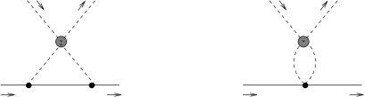
FIG. 2.: Long range contributions to the scalar and vector form factors.

In the work of Becher and Leutwyler [29] we can check that the only sources of $NN$ medium range effects are their diagrams $k$ and $l$, reproduced in figure 2, which contain two pions propagating in the $t$ channel. Here we consider explicitly their full contributions and our amplitudes $A_{R}^{\pm}$ and $B_{R}^{\pm}$ are written as

$$D_{R}^{+} = D_{mr}^{+}(t)+\left[\bar{d}_{00}^{+}+d_{10}^{+}\nu^{2}+\bar{d}_{01}^{+}t\right]_{(2)}+\left[d_{20}^{+}\nu^{4}+d_{11}^{+}\nu^{2}t+\bar{d}_{02}^{+}t^{2}\right]_{(3)}\;,$$ (32)

$$B_{R}^{+} = B_{mr}^{+}(t)+\left[b_{00}^{+}\nu\right]_{(1)}\;,$$ (33)

$$D_{R}^{-} = D_{mr}^{-}(t)+\left[\nu/(2f_{\pi}^{2})\right]_{(1)}+\left[\bar{d}_{00}^{-}\nu+d_{10}^{-}\nu^{3}+\bar{d}_{01}^{-}\nu t\right]_{(3)}\;,$$ (34)

$$B_{R}^{-} = B_{mr}^{-}(t)+\left[1/(2f_{\pi}^{2})+\bar{b}_{00}^{-}\right]_{(0)}+\left[b_{10}^{-}\nu^{2}+\bar{b}_{01}^{-}t\right]_{(1)}\;.$$ (35)

In these expressions, the labels $(n)$ outside the brackets indicate the presence of leading terms of ${\cal O}(q^{n})$, whereas the label $mr$ denotes the contribution from the medium range diagrams of fig.2. This decomposition implies the redefinition of some subthreshold coefficients, indicated by a bar over the appropriate symbol. Their explicit forms will be displayed in the sequence.

FIG. 3.: Dynamical structure of the ${\cal O}(q^{4})$ $\pi N$ amplitude; the blobs represent terms coming directly from the effective Lagrangians.

The dynamical content of the ${\cal O}(q^{4})$ $T_{\pi N}$ amplitude derived in [29] is shown in fig.3 and our approximation in fig.4. In the latter, the first two diagrams correspond to the direct and crossed PV Born amplitudes, with physical masses and coupling constants. The third one represents the contact interaction associated with the Weinberg-Tomozawa vertex, whereas the next two describe the medium range effects associated with the scalar and vector form factors. Finally, the last diagram summarizes the terms within square brackets in eqs.(32)–(35).

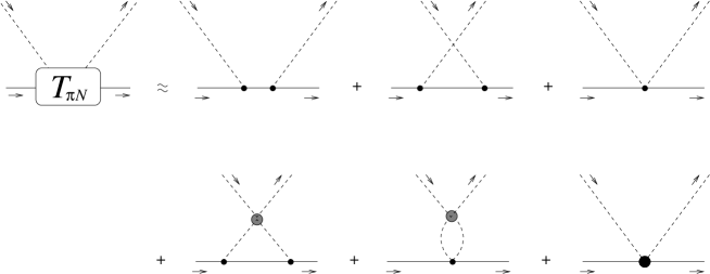
FIG. 4.: Dynamical content of the approximate $\pi N$ amplitude.

IV power counting

One begins the expansion of the TPEP to a given chiral order by recasting the explicitly covariant ${\cal T}_{T\!P}$ into the two-component form of eq.(23). This procedure involves no approximations and one finds, in the CM frame,

$$t_{C}^{\pm} = \tau^{\pm}\;\frac{m}{E}\left[\left(1\!+\!\mbox{\boldmath$q$}^{2}\!/\lambda^{2}\right)^{2}{\cal I}_{DD}^{\pm}-\frac{\mbox{\boldmath$q$}^{2}}{2m^{2}}\left(1\!+\!\mbox{\boldmath$q$}^{2}\!/\lambda^{2}\right)\left(1\!+\!\mbox{\boldmath$q$}^{2}\!/\lambda^{2}\!+\!\mbox{\boldmath$z$}^{2}\!/\lambda^{2}\right){\cal I}_{DB}^{(w)\pm}\right.$$ (36)

$$+ \left.\frac{\mbox{\boldmath$q$}^{4}}{16m^{4}}\left(1\!+\!\mbox{\boldmath$q$}^{2}\!/\lambda^{2}\!+\!\mbox{\boldmath$z$}^{2}\!/\lambda^{2}\right)^{2}{\cal I}_{BB}^{(w)\pm}+\frac{\mbox{\boldmath$q$}^{4}}{16m^{4}}\left(1\!+\!4m^{2}\mbox{\boldmath$z$}^{2}\!/\lambda^{4}\right){\cal I}_{BB}^{(g)\pm}\right.$$ (37)

$$- \left.\frac{\mbox{\boldmath$q$}^{2}\mbox{\boldmath$z$}^{2}}{2m^{2}\lambda^{2}}\left(1\!+\!\mbox{\boldmath$q$}^{2}\!/\lambda^{2}\right){\cal I}_{DB}^{(z)\pm}-\;\frac{\mbox{\boldmath$q$}^{4}\mbox{\boldmath$z$}^{4}}{16m^{4}\lambda^{4}}\;{\cal I}_{BB}^{(z)\pm}\right]\;,$$ (38)

$$t_{SS}^{\pm} = \tau^{\pm}\;\frac{m}{E}\left[-\;\frac{1}{6}\;{\cal I}_{BB}^{(g)\pm}\right]\;,$$ (39)

$$t_{T}^{\pm} = \tau^{\pm}\;\frac{m}{E}\left[-\;\frac{1}{12}\;{\cal I}_{BB}^{(g)\pm}\right]\;,$$ (40)

$$t_{LS}^{\pm} = \tau^{\pm}\;\frac{m}{E}\left[-\;\frac{4m^{2}}{\lambda^{2}}\left(1\!+\!\mbox{\boldmath$q$}^{2}\!/\lambda^{2}\right){\cal I}_{DD}^{\pm}+\left(1\!+\!2\mbox{\boldmath$q$}^{2}\!/\lambda^{2}\right)\left(1\!+\!\mbox{\boldmath$q$}^{2}\!/\lambda^{2}\!+\!\mbox{\boldmath$z$}^{2}\!/\lambda^{2}\right){\cal I}_{DB}^{(w)\pm}\right.$$ (41)

$$- \left.\frac{\mbox{\boldmath$q$}^{2}}{4m^{2}}\left(1\!+\!\mbox{\boldmath$q$}^{2}\!/\lambda^{2}\!+\!\mbox{\boldmath$z$}^{2}\!/\lambda^{2}\right)^{2}{\cal I}_{BB}^{(w)\pm}-\;\frac{\mbox{\boldmath$q$}^{2}}{4m^{2}}\left(1\!+\!4m^{2}\!/\lambda^{2}\!+\!4m^{2}\mbox{\boldmath$z$}^{2}\!/\lambda^{4}\right){\cal I}_{BB}^{(g)\pm}\right.$$ (42)

$$+ \left.\left(1\!+\!\mbox{\boldmath$q$}^{2}\!/\lambda^{2}\!+\!\mbox{\boldmath$z$}^{2}\!/\lambda^{2}+2\mbox{\boldmath$q$}^{2}\mbox{\boldmath$z$}^{2}/\lambda^{4}\right){\cal I}_{DB}^{(z)\pm}+\frac{\mbox{\boldmath$q$}^{2}\mbox{\boldmath$z$}^{2}}{4m^{2}\lambda^{2}}\left(1\!+\!\mbox{\boldmath$z$}^{2}\!/\lambda^{2}\right){\cal I}_{BB}^{(z)\pm}\right]\;,$$ (43)

$$t_{Q}^{\pm} = \tau^{\pm}\;\frac{m}{E}\left[-\;\frac{m^{4}}{\lambda^{4}}\;{\cal I}_{DD}^{\pm}+\frac{m^{2}}{2\lambda^{2}}\left(1\!+\!\mbox{\boldmath$q$}^{2}\!/\lambda^{2}\!+\!\mbox{\boldmath$z$}^{2}\!/\lambda^{2}\right){\cal I}_{DB}^{(w)\pm}\right.$$ (46)

$$\left.-\;\frac{1}{16}\left(1\!+\!\mbox{\boldmath$q$}^{2}\!/\lambda^{2}\!+\!\mbox{\boldmath$z$}^{2}\!/\lambda^{2}\right)^{2}{\cal I}_{BB}^{(w)\pm}-\;\frac{1}{16}\left(1\!+\!8m^{2}\!/\lambda^{2}\!+\!4m^{2}\mbox{\boldmath$z$}^{2}\!/\lambda^{4}\right){\cal I}_{BB}^{(g)\pm}\right.$$

$$\left.+\frac{m^{2}}{2\lambda^{2}}\left(1\!+\!\mbox{\boldmath$z$}^{2}\!/\lambda^{2}\right){\cal I}_{DB}^{(z)\pm}+\frac{1}{16}\left(1\!+\!\mbox{\boldmath$z$}^{2}\!/\lambda^{2}\right)^{2}{\cal I}_{BB}^{(z)\pm}\right]\;,$$

with $\mbox{\boldmath$q$}=\mbox{\boldmath$p$}^{\prime}\!-\!\mbox{\boldmath$p$}$, $\mbox{\boldmath$z$}=\mbox{\boldmath$p$}^{\prime}\!+\!\mbox{\boldmath$p$}$ and $\lambda^{2}=4m(E+m)$.

The potential to order ${\cal O}(q^{n})$ is determined by $t_{C}^{\pm}\rightarrow{\cal O}(q^{n})$, $\{t_{SS}^{\pm},t_{T}^{\pm},t_{LS}^{\pm}\}\rightarrow{\cal O}(q^{n\!-\!2})$ and $t_{Q}^{\pm}\rightarrow{\cal O}(q^{n\!-\!4})$. This means that one needs ${\cal I}_{DD}^{\pm}\rightarrow{\cal O}(q^{n})$, $\{{\cal I}_{DB}^{(w)\pm},{\cal I}_{DB}^{(z)\pm},{\cal I}_{BB}^{(g)\pm}\}\rightarrow{\cal O}(q^{n\!-\!2})$ and $\{{\cal I}_{BB}^{(w)\pm},{\cal I}_{BB}^{(z)\pm}\}\rightarrow{\cal O}(q^{n\!-\!4})$. We now discuss how the chiral powers in these functions are related with those in the basic $\pi N$ amplitude. This relationship involves a subtlety, associated with the fact that $D_{pv}^{+}$ and $B_{pv}^{-}$ contain chiral cancellations.

A generic subamplitude ${\cal I}_{XY}^{\pm}$ is given by the product of the corresponding $\pi N$ contributions and we have

$${\cal I}_{XY}^{\pm}=\int[\cdots]\left\{\left[X_{pv}^{\pm}\right]^{(1)}\!\left[Y_{pv}^{\pm}\right]^{(2)}\!\!+\!\left[X_{pv}^{\pm}\right]^{(1)}\!\left[Y_{R}^{\pm}\right]^{(2)}\!\!+\!\left[X_{R}^{\pm}\right]^{(1)}\!\left[Y_{pv}^{\pm}\right]^{(2)}\!\!+\!\left[X_{R}^{\pm}\right]^{(1)}\!\left[Y_{R}^{\pm}\right]^{(2)}\right\}\;.$$ (47)

The loop integral and the two pion propagators, as given by eq.(13), do not interfere with the counting of powers, since $\int[\cdots]\rightarrow{\cal O}(q^{0})$. The loop integration is symmetric under the operation $Q\rightarrow-Q$, which gives rise to the exchange $s\leftrightarrow u$ in the Born terms. In the case of $[X_{pv}^{\pm}]^{(1)}\;[Y_{pv}^{\pm}]^{(2)}$, one is allowed to use

$$\left(\frac{1}{s-m^{2}}\pm\frac{1}{u-m^{2}}\right)^{(i)}\left(\frac{1}{s-m^{2}}\pm\frac{1}{u-m^{2}}\right)^{(j)}\rightarrow 2\left(\frac{1}{s-m^{2}}\right)^{(i)}\left(\frac{1}{s-m^{2}}\pm\frac{1}{u-m^{2}}\right)^{(j)}$$ (48)

within the integrand. For the specific components this yields

$$\left[D_{pv}^{+}\right]^{(i)}\left[D_{pv}^{+}\right]^{(j)}\!\rightarrow{\cal O}(q^{3}),\;\;\;\;\; \left[D_{pv}^{-}\right]^{(i)}\left[D_{pv}^{-}\right]^{(j)}\!\rightarrow{\cal O}(q^{2}),$$ (49)

$$\left[D_{pv}^{+}\right]^{(i)}\left[QB_{pv}^{+}\right]^{(j)}\!\rightarrow{\cal O}(q),\;\;\;\;\; \left[D_{pv}^{-}\right]^{(i)}\left[QB_{pv}^{-}\right]^{(j)}\!\rightarrow{\cal O}(q),$$ (50)

$$\left[QB_{pv}^{+}\right]^{(i)}\left[QB_{pv}^{+}\right]^{(j)}\!\rightarrow{\cal O}(q^{0}),\;\;\;\;\; \left[QB_{pv}^{-}\right]^{(i)}\left[QB_{pv}^{-}\right]^{(j)}\!\rightarrow{\cal O}(q).$$ (51)

These results show that, inside the integral, $D_{pv}^{+}$ and $B_{pv}^{-}$ cannot be always counted as ${\cal O}(q^{2})$ and ${\cal O}(q^{-1})$, respectively. For the products $[X_{pv}^{\pm}]^{(i)}\;[Y_{R}^{\pm}]^{(j)}$ and $[X_{R}^{\pm}]^{(i)}\;[Y_{pv}^{\pm}]^{(j)}$, one uses

$$\left(\frac{1}{s-m^{2}}\pm\frac{1}{u-m^{2}}\right)^{(i)}\rightarrow 2\left(\frac{1}{s-m^{2}}\right)^{(i)}$$ (52)

and has $D_{pv}^{\pm}\rightarrow{\cal O}(q)$ and $B_{pv}^{\pm}\rightarrow{\cal O}(q^{-1})$. Assuming $[X_{R}^{\pm}]^{(i)},[Y_{R}^{\pm}]^{(j)}\rightarrow{\cal O}(q^{r})$, one gets

$$\left[D_{pv}^{\pm}\right]^{(i)}\left[D_{R}^{\pm}\right]^{(j)}\!\rightarrow{\cal O}(q^{1+r}),\;\;\;\;\; \left[D_{pv}^{\pm}\right]^{(i)}\left[QB_{R}^{\pm}\right]^{(j)}\!\rightarrow{\cal O}(q^{2+r}),$$ (53)

$$\left[D_{R}^{\pm}\right]^{(i)}\left[QB_{pv}^{\pm}\right]^{(j)}\!\rightarrow{\cal O}(q^{r}),\;\;\;\;\; \left[QB_{pv}^{\pm}\right]^{(i)}\left[QB_{R}^{\pm}\right]^{(j)}\!\rightarrow{\cal O}(q^{1+r}).$$ (54)

Finally, in the case of $[X_{R}^{\pm}]^{(i)}[Y_{R}^{\pm}]^{(j)}$, one just adds the corresponding powers.

In this work we consider the expansion of the potential to ${\cal O}(q^{4})$ and need ${\cal I}_{DD}^{\pm}\rightarrow{\cal O}(q^{4})$, $\{{\cal I}_{DB}^{(w)\pm},{\cal I}_{DB}^{(z)\pm},{\cal I}_{BB}^{(g)\pm}\}\rightarrow{\cal O}(q^{2})$, and $\{{\cal I}_{BB}^{(w)\pm},{\cal I}_{BB}^{(z)\pm}\}\rightarrow{\cal O}(q^{0})$. This means that, in the intermediate $\pi N$ amplitude, we must consider $D_{R}^{\pm}$ to ${\cal O}(q^{3})$ and $B_{R}^{\pm}$ to ${\cal O}(q)$.

V subthreshold coefficients

The polynomial parts of the amplitudes $T_{R}^{\pm}$ to order ${\cal O}(q^{3})$, as given by eqs.(30)–(33), are determined by the subthreshold coefficients of ref. [29], which we reproduce below

$$d_{00}^{+} = -\frac{2\;(2c_{1}-c_{3})\;\mu^{2}}{f_{\pi}^{2}}+\frac{8\;g_{A}^{4}\;\mu^{3}}{64\;\pi\;f_{\pi}^{4}}+\left[\frac{3\;g_{A}^{2}\;\mu^{3}}{64\;\pi\;f_{\pi}^{4}}\right]_{mr}\;,$$ (55)

$$d_{10}^{+} = \frac{2\;c_{2}}{f_{\pi}^{2}}-\frac{(4+5\;g_{A}^{4})\;\mu}{32\;\pi\;f_{\pi}^{4}}\;,$$ (56)

$$d_{01}^{+} = -\frac{c_{3}}{f_{\pi}^{2}}-\frac{48\;g_{A}^{4}\;\mu}{768\;\pi\;f_{\pi}^{4}}-\left[\frac{77\;g_{A}^{2}\;\mu}{768\;\pi\;f_{\pi}^{4}}\right]_{mr}\;,$$ (57)

$$d_{20}^{+} = \frac{12+5\;g_{A}^{4}}{192\;\pi\;f_{\pi}^{4}\;\mu}\;,$$ (58)

$$d_{11}^{+} = \frac{g_{A}^{4}}{64\;\pi\;f_{\pi}^{4}\;\mu}\;,$$ (59)

$$d_{02}^{+} = \left[\frac{193\;g_{A}^{2}}{15360\;\pi\;f_{\pi}^{4}\;\mu}\right]_{mr}\;,$$ (60)

$$b_{00}^{+} = \frac{4\;m\;(\tilde{d}_{14}-\tilde{d}_{15})}{f_{\pi}^{2}}-\frac{g_{A}^{4}\;m}{8\;\pi^{2}\;f_{\pi}^{4}}\;,$$ (61)

$$d_{00}^{-} = \left[\frac{1}{2\;f_{\pi}^{2}}\right]_{WT}+\frac{4\;(\tilde{d}_{1}+\tilde{d}_{2}+2\;\tilde{d}_{5})\;\mu^{2}}{f_{\pi}^{2}}+\frac{g_{A}^{2}\;(-3+g_{A}^{2})\;\mu^{2}}{48\;\pi^{2}\;f_{\pi}^{4}}+\left[\frac{3\;g_{A}^{2}\;\mu^{2}}{48\;\pi^{2}\;f_{\pi}^{4}}\right]_{mr}\;,$$ (62)

$$d_{10}^{-} = \frac{4\;\tilde{d}_{3}}{f_{\pi}^{2}}-\frac{15+7\;g_{A}^{4}}{240\;\pi^{2}\;f_{\pi}^{4}}\;,$$ (63)

$$d_{01}^{-} = -\frac{2\;(\tilde{d}_{1}+\tilde{d}_{2})}{f_{\pi}^{2}}-\frac{2\;g_{A}^{4}}{192\;\pi^{2}\;f_{\pi}^{4}}-\left[\frac{1+7\;g_{A}^{2}}{192\;\pi^{2}\;f_{\pi}^{4}}\right]_{mr}\;,$$ (64)

$$b_{00}^{-} = \left[\frac{1}{2\;f_{\pi}^{2}}\right]_{WT}+\frac{2\;c_{4}\;m}{f_{\pi}^{2}}-\frac{g_{A}^{4}\;m\;\mu}{8\;\pi\;f_{\pi}^{4}}-\left[\frac{g_{A}^{2}\;m\;\mu}{8\;\pi\;f_{\pi}^{4}}\right]_{mr}\;,$$ (65)

$$b_{10}^{-} = \frac{g_{A}^{4}\;m}{32\;\pi\;f_{\pi}^{4}\;\mu}\;,$$ (66)

$$b_{01}^{-} = \left[\frac{g_{A}^{2}\;m}{96\;\pi\;f_{\pi}^{4}\;\mu}\right]_{mr}\;,$$ (67)

where the parameters $c_{i}$ and $\tilde{d}_{i}$ are the usual renormalized coupling constants of the chiral Lagrangians of order 2 and 3, respectively [26]. The terms within square brackets labelled $(mr)$ in some of these results are due to the medium range diagrams shown in fig.2 and must be neglected, because we already include their contributions in $D_{mr}^{\pm}$ and $B_{mr}^{\pm}$. The terms bearing the $(W\!T)$ label must also be excluded, for they were explicitly considered in eqs.(32)–(35). This corresponds to the redefinition mentioned at the end of section III.

TABLE I.: experimental values for the subthreshold coefficients and medium range (mr) contributions in $\mu^{-n}$ units; experimental results are taken from ref. [REFERENCES].

	$d_{00}^{+}$	$d_{10}^{+}$	$d_{01}^{+}$	$d_{20}^{+}$	$d_{11}^{+}$	$d_{02}^{+}$
exp	-1.46$\pm$0.10	1.12$\pm$0.02	1.14$\pm$0.02	0.200$\pm$0.005	0.17$\pm$0.01	0.036$\pm$0.003
mr	0.12	-	-0.25	-	-	0.032
	$b_{00}^{+}$
exp	-3.54$\pm$0.06
	$d_{00}^{-}$	$d_{10}^{-}$	$d_{01}^{-}$
exp	1.53$\pm$0.02	-0.167$\pm$0.005	-0.134$\pm$0.005
$W\!T+mr$	1.18	-	-0.032
	$b_{00}^{-}$	$b_{10}^{-}$	$b_{01}^{-}$
exp	10.36$\pm$0.10	1.08 $\pm$0.05	0.24$\pm$0.01
$W\!T+mr$	-0.99	-	0.18

The values of the subthreshold coefficients are determined from $\pi N$ scattering data and, in a chiral expansion to ${\cal O}(q^{3})$, they are used to fix the otherwise undetermined parameters $c_{i}$ and $\tilde{d}_{i}$. In our formulation of the TPEP, we bypass the use of these unknown parameters, for the redefined subthreshold coefficients are already the dynamical ingredients that determine the strength of the various interactions. This allows the potential to be expressed directly in terms of observable quantities.

In table I we show the experimental values of the subthreshold coefficients determined in ref. [16] and the sum of $(W\!T)$ and $(mr)$ contributions. The redefined values are obtained by just subtracting the latter from the former. It is worth noting that the values of $\bar{d}_{02}^{+}$ and $\bar{b}_{01}^{-}$ are compatible with zero.

When writing the results for the TPEP, it is very convenient to display explicitly the chiral scales of the various contributions. With this purpose in mind, we will employ the dimensionless subthreshold constants defined in table II.

TABLE II.: Dimensionless subthreshold coefficients.

	$\bar{\delta}_{00}^{+}$	$\delta_{10}^{+}$	$\bar{\delta}_{01}^{+}$	$\beta_{00}^{+}$
definition	$mf_{\pi}^{2}\;d_{00}^{+}/\mu^{2}$	$mf_{\pi}^{2}\;d_{10}^{+}$	$mf_{\pi}^{2}\;d_{01}^{+}$	$mf_{\pi}^{2}\;b_{00}^{+}$
value	-4.72	3.34	4.15	-10.57
	$\bar{\delta}_{00}^{-}$	$\delta_{10}^{-}$	$\bar{\delta}_{01}^{-}$	$\bar{\beta}_{00}^{-}$
definition	$m^{2}f_{\pi}^{2}\;\bar{d}_{00}^{-}/\mu^{2}$	$m^{2}f_{\pi}^{2}\;d_{10}^{-}$	$m^{2}f_{\pi}^{2}\;\bar{d}_{01}^{-}$	$f_{\pi}^{2}\;\bar{b}_{00}^{-}$
value	7.02	-3.35	-2.05	5.04

VI relativistic and heavy baryon formulations

In this section we review briefly the relativistic formulation of baryon ChPT and its relationship with the widely used heavy baryon techniques. Chiral perturbation theory is a systematic expansion of low-energy amplitudes in powers of momenta and quark masses, generically denoted by $q$. The chiral Lagrangian consists of a string of terms, labeled by its power in $q$. To a given order, one builds the most general Lagrangian, consistent with Poincaré invariance and other symmetries of QCD (parity, time reversal, and approximate chiral symmetry). A Lagrangian of order $n$ produces tree graphs of the same order, while loop graphs are expected to contribute at higher orders, following a power counting scheme. This is indeed what happens in the mesonic sector, where loop graphs are two orders higher than tree graphs, if one uses dimensional regularization.

In relativistic baryon ChPT, dimensional regularization no longer leads to a well defined power counting [33], loops start at the same order as tree graphs and the connection between loop and momentum expansion is lost. A similar phenomenon is observed in the mesonic sector if one uses another regularization scheme, such as Pauli-Villars.

In HBChPT, this problem is overcome by means of the expansion of the original Lagrangian around the infinite nucleon mass limit [38]. One integrates out the heavy degrees of freedom of the nucleon field, eliminates its mass $m$ from the propagator, and expands the resulting vertices in powers of $1/m$. This formulation gives rise to a power counting scheme, but Lorentz invariance is no longer explicit. It can still be recovered, but only after a resummation of all terms in this expansion.

The HB approach also has a more serious problem, pointed out recently by Becher and Leutwyler [28], namely, that it fails to converge in part of the low-energy region. In order to avoid this, they proposed a new regularization scheme, the so called Infrared Regularization, which is manifestly Lorentz invariant and gives rise to a power counting. The method is based on a previous work by Ellis and Tang [31], where a loop integral $H$ was separated into “soft”, infrared ($I$) and “hard”, regular ($R$) pieces. The former satisfies a power counting rule and has the same analytic structure as $H$ in the low-energy domain. The latter may contain singularities only at high energies — in the low-energy region, it is well behaved and can be expanded in a Taylor series, resulting in polynomials of the generic momentum $q$. Therefore the hard pieces, which are the power counting violating terms, can be absorbed in the appropriate coupling constants of the Lagrangian and one considers only $I$, the infrared-regularized part of $H$.

Ellis and Tang have shown that the chiral expansion of the infrared regularized one-loop integral $I$, with the ratio $q/\mu$ fixed, reproduces formally the corresponding terms in the HBChPT approach [31], even in the cases where such an expansion is not permitted. This allows one to assess the domain of validity of the HB series.

For the sake of completeness, in the sequence, we reproduce some of the results derived by Becher and Leutwyler. They have analyzed in detail the triangle graph of fig.4, which contributes to the nucleon scalar form factor, and shown that the HBChPT formulation is not suited for the low energy-region, near $t=4\mu^{2}$. Its exact spectral representation is given by [33]

$$\gamma(t)=\frac{1}{\pi}\int_{4\mu^{2}}^{\infty}\frac{dt^{\prime}}{(t^{\prime}-t)}\,\mbox{Im}\gamma(t^{\prime})\;,$$ (68)

where

$$\mbox{Im}\gamma(t^{\prime}) = \frac{\theta(t^{\prime}-4\mu^{2})}{8\pi m\sqrt{t^{\prime}(4m^{2}-t^{\prime})}}\,\tan^{-1}\frac{\sqrt{(4m^{2}-t^{\prime})(t^{\prime}-4\mu^{2})}}{t^{\prime}-2\mu^{2}}$$ (69)

$$\simeq \frac{\theta(t^{\prime}-4\mu^{2})}{16\pi m\sqrt{t^{\prime}}}\,\tan^{-1}\frac{2m\sqrt{t^{\prime}-4\mu^{2}}}{t^{\prime}-2\mu^{2}}\,.$$ (70)

Formally, the argument

$$x=\frac{2m\sqrt{t^{\prime}-4\mu^{2}}}{t^{\prime}-2\mu^{2}}$$ (71)

seems to be of order $q^{-1}$, and the HB chiral expansion of (70) would yield $\tan^{-1}x=\pi/2-1/x+1/3x^{3}+\cdots$. However, this representation of $\tan^{-1}x$ is valid only in the domain $|x|\geq 1$. For $|x|<1$, one should use $\tan^{-1}x=x-x^{3}/3+\cdots$, but this corresponds to an expansion in inverse powers of $q$. From (71) we see that the HB expansion of (68) breaks down when $t^{\prime}$ approaches $4\mu^{2}$.

Becher and Leutwyler have shown that it is possible to write accurately

$$\gamma(t)-\gamma(0) = \frac{t}{\pi}\int_{4\mu^{2}}^{\infty}\frac{dt^{\prime}}{t^{\prime}(t^{\prime}-t)}\,\frac{1}{16\pi m\sqrt{t^{\prime}}}\left\{\left[\frac{\pi}{2}-\frac{(t^{\prime}-2\mu^{2})}{2m\sqrt{t^{\prime}\!-\!4\mu^{2}}}\right]_{\!HB}\right.$$ (72)

$$+ \left.\left[\frac{\mu\sqrt{t^{\prime}}}{2m\sqrt{t^{\prime}\!-\!4\mu^{2}}}-\frac{\sqrt{t^{\prime}}}{2\mu}\tan^{-1}\frac{\mu^{2}}{m\sqrt{t^{\prime}\!-\!4\mu^{2}}}\right]_{\!t\!h}\right\}\;.$$ (73)

By keeping only the first bracket in the integrand, one recovers the heavy baryon result. However, the region $t\sim 4\mu^{2}$ is dominated by the lower end of integration in $t^{\prime}$, where the second term becomes important. The HB approximation is not valid there. The integration can be performed analytically and Becher and Leutwyler found

$$\gamma(t)-\gamma(0) = \frac{1}{32\pi m\mu}\left\{\left[\frac{1}{\sqrt{\tau}}\ln\frac{2+\sqrt{\tau}}{2-\sqrt{\tau}}-1+\frac{2\mu(2-\tau)}{\pi m\sqrt{\tau(4-\tau)}}\sin^{-1}\frac{\sqrt{\tau}}{2}-\frac{\mu}{\pi m}\right]_{\!HB}\right.$$ (74)

$$+ \left.\left[\frac{\mu}{m\sqrt{4-\tau}}-\frac{\mu}{2m}-\ln\left(1+\frac{\mu}{m\sqrt{4-\tau}}\right)+\ln\left(1+\frac{\mu}{2m}\right)\right]_{\!t\!h}\right\}$$ (75)

with $\tau=t/\mu^{2}$. This result is interesting because it shows clearly that, for values of $t$ far from $4\mu^{2}$, the contributions of the two brackets decouple and can be expanded in powers of $q$. The second term is then ${\cal O}(q^{2})$. On the other hand, when $t\sim 4\mu^{2}$, both contributions merge, the full result for $\gamma(t)$ is the outcome of large cancellations between them, and an expansion in $q$ does not apply. In fig.5, we display the behavior of the various terms in eq.(75) in the range $3.5\mu^{2}\leq t\leq 4\mu^{2}$, where the second bracket is important. In this figure we also show the effect of making

$$\left[\frac{\mu}{m\sqrt{4-\tau}}-\frac{\mu}{2m}-\ln\left(1+\frac{\mu}{m\sqrt{4-\tau}}\right)+\ln\left(1+\frac{\mu}{2m}\right)\right]_{\!t\!h}\rightarrow\frac{\mu^{2}}{m^{2}(4-\tau)}-\frac{\mu^{2}}{4m^{2}}\;.$$ (76)

This rough approximation is not mathematically precise, but it allows one to guess the order of magnitude of the threshold contribution.

FIG. 5.: Behavior of the function $\gamma(t)$ as given by eq.(75) (full line) and partial contributions: HB (dashed line), $th$ (dotted line) and eq.(76) (dot-dashed line).

The discussion of the behavior of the triangle diagram in the neighborhood of $t=4\mu^{2}$ is relevant to the $NN$ potential because, in configuration space, this region describes its long distance properties, as observed numerically in our previous works [20, 32]. To see this, let us take the representation of (68) in configuration space:

$$\Gamma(r)=\frac{1}{\pi}\int_{4\mu^{2}}^{\infty}dt^{\prime}\int\frac{d^{3}q}{(2\pi)^{3}}\;e^{-i{\mbox{\boldmath$q$}}\cdot{\mbox{\boldmath$r$}}}\;\frac{\mbox{Im}\gamma(t^{\prime})}{t^{\prime}+{\mbox{\boldmath$q$}}^{2}}=\frac{1}{4\pi^{2}}\int_{4\mu^{2}}^{\infty}dt^{\prime}\;\frac{e^{-r\sqrt{t^{\prime}}}}{r}\;\,\mbox{Im}\gamma(t^{\prime})\,.$$ (77)

The exponential in the integrand shows clearly that, for large values of $r$, results are dominated by the lower end of the integration. Thus, if we want to have a good description of $\Gamma(r)$ at large distances, we need a decent representation for $\mbox{Im}\gamma(t^{\prime})$ near $t^{\prime}=4\mu^{2}$, which is not provided by HBChPT.

VII dynamics

The chiral two-pion exchange potential is determined by the processes depicted in fig.6, derived from the basic $\pi N$ subamplitude and organized into three different families. The first one corresponds to the minimal realization of chiral symmetry [14], includes the subtraction of the iterated OPEP, and involves only pion-nucleon interactions with a single loop, associated with the constants $m$, $g$, and $f_{\pi}$. The same constants also determine the two-loop processes of the second family. The last family includes chiral corrections associated with subthreshold coefficients and LECs, representing either higher order processes or other degrees of freedom.

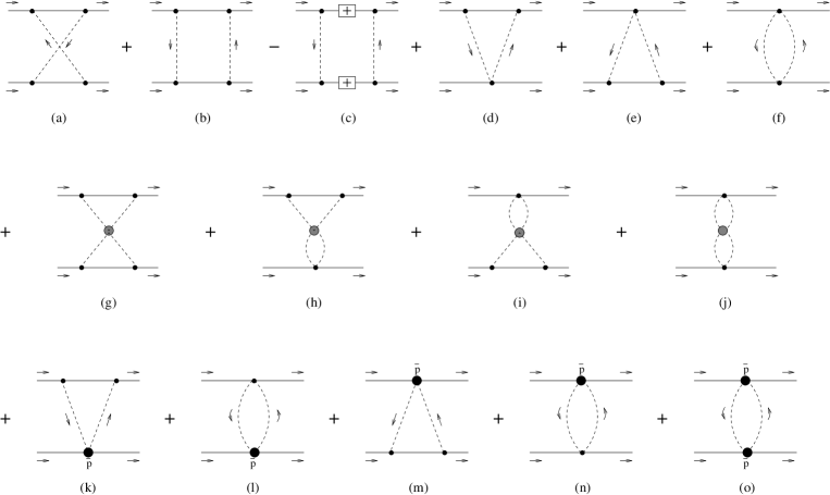
FIG. 6.: Dynamical structure of the TPEP. The first two diagrams correspond to the products of Born $\pi N$ amplitudes, the third one represents the iteration of the OPEP, whereas the next three involve contact interactions associated with the Weinberg-Tomozawa vertex. The diagrams on the second line describe medium range effects associated with scalar and vector form factors. The remaining interactions are triangles and bubbles involving subthreshold coefficients.

The first two diagrams of fig.6, known, respectively, as crossed box and box, come from the products of the $\pi N$ PV Born amplitudes, given by eqs.(25)–(28) and involve the propagations of two pions and two nucleons. The third one represents the iteration of the OPEP and gives rise to an amplitude denoted by ${\cal T}_{it}$, derived after the work of Partovi and Lomon [5] and discussed in detail in appendix C. The remaining interactions correspond to triangle and bubble diagrams, which contain a single or no nucleon propagators, besides those of two pions.

The construction of the TPEP begins with the determination of the relativistic profile functions, eqs.(9)–(12), using the $\pi N$ subamplitudes $D^{\pm}$ and $B^{\pm}$ discussed in section III. Results are then expressed in terms of the one-loop Feynman integrals presented in appendixes B and C, which may involve two, three, or four propagators. The evaluation and manipulation of these integrals represent an important aspect of the present work and it is worth discussing the notation employed.

Momentum space integrals are generally denoted by $\Pi$ and labeled in such a way as to recall their dynamical origins. We use lower labels, corresponding to nucleons 1 and 2, with the following meanings: $c\rightarrow$ contact interaction; $s\rightarrow$ $s$-channel nucleon propagation; and $u\rightarrow$ $u$-channel nucleon propagation. This means that functions carrying the subscripts $(cc)$, $(sc)$, $(ss)$, and $(us)$ correspond, respectively, to bubble, triangle, crossed box, and box diagrams. The last class of integrals includes the OPEP cut, which needs to be subtracted. This subtraction is implemented by replacing the $(us)$ integrals by regular ones, represented by the subscript $(reg)$ and given in appendix C. Upper labels, on the other hand, indicate the rank of the integral in the external kinematical variables $q,z$ and $W$. For instance, the rank 2 crossed box integral is written as

$$I_{ss}^{\mu\nu} = \int\frac{d^{4}Q}{(2\pi)^{2}}\;\left(\frac{Q^{\mu}Q^{\nu}}{\mu^{2}}\right)\frac{1}{k^{2}-\mu^{2}}\;\frac{1}{k^{\prime 2}-\mu^{2}}\;\frac{2m\mu}{s_{1}-m^{2}}\;\frac{2m\mu}{s_{2}-m^{2}}$$ (78)

$$= \frac{i}{(4\pi)^{2}}\left[\frac{q^{\mu}q^{\nu}}{\mu^{2}}\;\Pi_{ss}^{(200)}+\frac{z^{\mu}z^{\nu}}{4m^{2}}\;\Pi_{ss}^{(020)}+\frac{W^{\mu}W^{\nu}}{4m^{2}}\;\Pi_{ss}^{(002)}+g^{\mu\nu}\;\bar{\Pi}_{ss}^{(000)}\right]\;.$$ (79)

All integrals are dimensionless and include suitable powers of pion and nucleon masses, so as to make them relatively stable upon wide variations of the latter. We have studied these integrals numerically and, typically, they change by 30% when one moves the nucleon mass from its empirical value to infinity. The fact that the integrals are ${\cal O}(q^{0})$ is rather useful in discussing chiral scales and heavy baryon limits. At present the infrared regularization techniques are still being developed for the case of two nucleon system [39] and we have used dimensional regularization whenever appropriate. As a consequence, our results are accurate only for distances larger than a typical radius. Our numerical studies in configuration space indicate that this radius is of about 1 fm.

The covariantly expanded TPEP, to be given in section X, is expressed in terms of the functions $\Pi_{cc}^{(000)}$, $\Pi_{sc}^{(000)}$, $\Pi_{ss}^{(000)}$, $\Pi_{reg}^{(000)}$, and $\Pi_{reg}^{(010)}$. In order to simplify the notation, in the main text we call them $\Pi_{\ell}$, $\Pi_{t}$, $\Pi_{\times}$, $\Pi_{b}$, and $\tilde{\Pi}_{b}$, respectively.

The function $\Pi_{\ell}$ represents the bubble diagram and is given by

$$I_{cc}=\int\frac{d^{4}Q}{(2\pi)^{4}}\;\frac{1}{[k^{2}\!-\!\mu^{2}][k^{\prime 2}\!-\!\mu^{2}]}=\frac{i}{(4\pi)^{2}}\;\Pi_{\ell}\;.$$ (80)

This integral can be performed analitically and its regular part may be written as

$$\Pi_{\ell}=-2\;\frac{\sqrt{1-t/4\mu^{2}}}{\sqrt{-t/4\mu^{2}}}\;\ln\left(\sqrt{1-t/4\mu^{2}}+\sqrt{-t/4\mu^{2}}\right)\;.$$ (81)

The function $\Pi_{t}$, associated with the triangle diagram, is expressed by

$$I_{sc}=\int\frac{d^{4}Q}{(2\pi)^{4}}\;\frac{1}{[k^{2}\!-\!\mu^{2}][k^{\prime 2}\!-\!\mu^{2}]}\;\frac{2m\mu}{[s_{1}-m^{2}]}=\frac{i}{(4\pi)^{2}}\;\Pi_{t}$$ (82)

and related to the function $\gamma(t)$ discussed in the preceding section by $\Pi_{t}=-2m\mu(4\pi)^{2}\gamma(t)$. The heavy-baryon representation of this function is

$$\Pi_{t}\rightarrow\Pi_{t}^{\!H\!B}=\Pi_{a}+\frac{\mu}{2m}\;\Pi_{t}^{N\!\!L}$$ (83)

with

$$\Pi_{a} = -\;\frac{\pi}{\sqrt{-t/4\mu^{2}}}\tan^{-1}\sqrt{-t/4\mu^{2}}\;,$$ (84)

$$\Pi_{t}^{N\!\!L} = (1\!-\!t/2\mu^{2})\;\Pi^{\prime}_{\ell}\;,$$ (85)

and $\Pi^{\prime}=\mu\;(d\Pi/d\mu)$.

The functions $\Pi_{\times}$, $\Pi_{b}$, and $\tilde{\Pi}_{b}$ are associated with crossed box and box diagrams and their complete expressions are given in appendix B. Their heavy baryon expansions are derived in appendix G and read

$$\Pi_{\times}^{\!H\!B}=-\Pi^{\prime}_{\ell}-\left[\frac{\mu}{m}\right]\frac{\pi/2}{(1\!-\!t/4\mu^{2})}-\left[\frac{\mu}{m}\right]^{2}\frac{1}{4}\;\left[(1\!-\!t/2\mu^{2})^{2}\left(2\;\Pi^{\prime}_{\ell}-\Pi^{\prime\prime}_{\ell}\right)+(2z^{2}/3\mu^{2})\;\Pi^{\prime}_{\ell}\right]+\cdots\;,$$ (86)

$$\Pi_{b}^{\!H\!B}=\Pi_{\times}^{\!H\!B}+\left[\frac{\mu}{m}\right]\frac{\pi/4}{(1\!-\!t/4\mu^{2})}+\left[\frac{\mu}{m}\right]^{2}\frac{1}{6}\;\left[(1\!-\!t/2\mu^{2})^{2}\left(2\;\Pi^{\prime}_{\ell}-\Pi^{\prime\prime}_{\ell}\right)\right]+\cdots\;,$$ (87)

$$\tilde{\Pi}_{b}^{\!H\!B}=-\;\frac{1}{2}\;\Pi_{a}-\left[\frac{\mu}{m}\right]\frac{1}{3}\;(1\!-\!t/2\mu^{2})\;\Pi^{\prime}_{\ell}+\cdots\;.$$ (88)

In the heavy baryon expansion of the potential, the following results are useful

$$\Pi^{\prime}_{\ell}=2+\Pi_{\ell}/(1\!-\!t/4\mu^{2})\;,$$ (89)

$$\Pi^{\prime\prime}_{\ell}=2/(1\!-\!t/4\mu^{2})+\left[2/(1\!-\!t/4\mu^{2})-1/(1\!-\!t/4\mu^{2})^{2}\right]\Pi_{\ell}\;,$$ (90)

$$\Pi_{a}^{\prime}=\Pi_{a}-\pi\,t/(1-t/4\mu^{2})\;.$$ (91)

For the reasons discussed in the preceding section, all these heavy baryon representations are inaccurate around $t\sim 4\mu^{2}$.

VIII covariant amplitudes

The direct reading of the Feynman diagrams of fig.6 gives rise to our full results for the relativistic profile functions, displayed in appendix D. These are the functions that the chiral expansion must converge to and hence they allow one to assess the series directly. On the other hand, they do not exhibit explicitly the chiral scales of the various components of the potential, since their net values are the outcome of several cancellations.

In order to display these scales, in appendix E we derive several relations among integrals, which are used to transform the full results of appendix D into the forms listed in appendix F. The relations given in appendix E are, in principle, exact, provided one keeps short range integrals that contain a single or no pion propagators. However, for the sake of simplicity, we neglect those contributions. The importance of this approximation was checked by comparing numerically the Fourier transforms of the various amplitudes of appendixes D and F. In all cases, agreement is much better than 1% for distances larger than 1 fm, except for ${\cal I}_{DD}^{+}$, where the difference is 4% at 1.5 fm and falls below 1% beyond 2.5 fm. This has very little influence over the full potential.

With the purpose of allowing comparison with results produced in the HB tradition, we write our final expressions for the potential in terms of the axial constant $g_{A}$, which is related to the $\pi N$ coupling constant by $g=\left(1+\Delta_{GT}\right)\;g_{A}m/f_{\pi}$. Here $\Delta_{GT}$ is the Goldberger-Treiman (GT) discrepancy, proportional to $\mu^{2}$. In applications, on the other hand, we recommend the direct use of the $\pi N$ coupling constant $g$, by making $g_{A}=gf_{\pi}/m$ and neglecting $\Delta_{GT}$ in our results.

The appropriate truncation of the expressions of appendix F, at the orders in $q$ prescribed at the end of section IV, leads to the following results for the profile functions:

$$\bullet {\cal I}_{DD}^{+}=\frac{m^{2}}{16\;\pi^{2}f_{\pi}^{4}}\;\left[\frac{\mu}{m}\right]^{2}\left\{\frac{g_{A}^{4}}{16}\;(1\!-\!t\!/2\mu^{2})^{2}\left(\Pi_{\times}-\Pi_{b}\right)+\Delta_{GT}\,\frac{g_{A}^{4}}{4}\;(1\!-\!t\!/2\mu^{2})^{2}\left(\Pi_{\times}-\Pi_{b}\right)\right.$$ (95)

$$\left.+\left[\frac{\mu}{m}\right]\frac{g_{A}^{2}}{8}\;(1\!-\!t\!/2\mu^{2})\left[-g_{A}^{2}\;\Pi_{a}+4\left(\bar{\delta}_{00}^{+}+\bar{\delta}_{01}^{+}\;t/\mu^{2}\right)\Pi_{t}\right]+\left[\frac{\mu}{m}\right]^{2}\left[-\frac{g_{A}^{2}}{4}\;\delta_{10}^{+}\;(1\!-\!t\!/2\mu^{2})^{2}\right.\right.$$

$$\left.\left.+\frac{1}{2}\left(\bar{\delta}_{00}^{+}+\bar{\delta}_{01}^{+}\;t/\mu^{2}+\frac{1}{3}\;\delta_{10}^{+}\;(1\!-\!t\!/4\mu^{2})\right)^{2}+\frac{2}{45}\left(\delta_{10}^{+}\right)^{2}(1\!-\!t\!/4\mu^{2})^{2}\right]\Pi_{\ell}\right.$$

$$\left.-\left[\frac{\mu}{m}\right]^{2}\;\frac{m^{2}}{256\;\pi^{2}f_{\pi}^{2}}\;g_{A}^{4}\;(1\!-\!2t\!/\mu^{2})\left[(1\!-\!t\!/2\mu^{2})\;\Pi_{t}-2\pi\right]^{2}\right\}\;,$$

$$\bullet {\cal I}_{DB}^{(w)+}=\frac{m^{2}}{16\;\pi^{2}f_{\pi}^{4}}\;\left[\frac{\mu}{m}\right]\left\{-\frac{g_{A}^{4}}{8}\;(1\!-\!t\!/2\mu^{2})\;\Pi_{t}\right.$$ (97)

$$\left.+\left[\frac{\mu}{m}\right]\left[\frac{g_{A}^{4}}{16}\;(1\!-\!t\!/2\mu^{2})^{2}\;\Pi_{\times}-\frac{g_{A}^{2}}{2}\left(\bar{\delta}_{00}^{+}+\bar{\delta}_{01}^{+}\;t/\mu^{2}+\frac{1}{3}\;\delta_{10}^{+}\;(1\!-\!t\!/4\mu^{2})\right)\Pi_{\ell}\right]\right\}\;,$$

$$\bullet {\cal I}_{DB}^{(z)+}=\frac{m^{2}}{16\;\pi^{2}f_{\pi}^{4}}\;\left[\frac{\mu}{m}\right]\left\{\frac{g_{A}^{4}}{8}\left[(1\!-\!t\!/2\mu^{2})\;\tilde{\Pi}_{b}-(3/2\!-\!5t\!/8\mu^{2})\;\Pi_{a}\right]\right.$$ (99)

$$\left.+\left[\frac{\mu}{m}\right]\frac{g_{A}^{2}}{2}\left(\bar{\delta}_{00}^{+}+\bar{\delta}_{01}^{+}\;t/\mu^{2}-\delta_{10}^{+}\;(1\!-\!t\!/4\mu^{2})\right)\Pi_{\ell}\right\}\;,$$

$$\bullet {\cal I}_{BB}^{(g)+}=\frac{m^{2}}{16\;\pi^{2}f_{\pi}^{4}}\left\{\frac{g_{A}^{4}}{4}\;(1\!-\!t/4\mu^{2})\left(\Pi_{\times}+\Pi_{b}\right)+\Delta_{GT}\;g_{A}^{4}\;(1\!-\!t/4\mu^{2})\left(\Pi_{\times}+\Pi_{b}\right)\right.$$ (102)

$$\left.+\left[\frac{\mu}{m}\right]\frac{g_{A}^{4}}{8}\left[(1\!-\!t\!/2\mu^{2})\left(\Pi_{t}-\tilde{\Pi}_{b}\right)+(1\!-\!t/4\mu^{2})\;\Pi_{a}\right]\right.$$

$$\left.-\left[\frac{\mu}{m}\right]^{2}g_{A}^{2}\left[\frac{g_{A}^{2}}{16}\;(1\!-\!t\!/2\mu^{2})^{2}\;\Pi_{\times}+\frac{1}{3}\;\beta_{00}^{+}\;(1\!-\!t\!/4\mu^{2})\;\Pi_{\ell}\right]\right\}\;,$$

$$\bullet {\cal I}_{BB}^{(w)+}=\frac{m^{2}}{16\;\pi^{2}f_{\pi}^{4}}\;g_{A}^{4}\;\Pi_{\ell}\;,$$ (103)

$$\bullet {\cal I}_{BB}^{(z)+}=\frac{m^{2}}{16\;\pi^{2}f_{\pi}^{4}}\;\frac{g_{A}^{4}}{3}\;\Pi_{\ell}\;,$$ (104)

and

$$\bullet {\cal I}_{DD}^{-}=\frac{m^{2}}{16\;\pi^{2}f_{\pi}^{4}}\left[\frac{\mu}{m}\right]^{2}\left\{\frac{g_{A}^{4}}{16}\;(1\!-\!t/2\mu^{2})^{2}\left(\Pi_{\times}+\Pi_{b}\right)-\frac{g_{A}^{2}}{4}\;(g_{A}^{2}-1)\;(1\!-\!t/2\mu^{2})\;\Pi_{\ell}\right.$$ (113)

$$\left.+\frac{1}{24}\;(g_{A}^{2}-1)^{2}(1\!-\!t/4\mu^{2})\;\Pi_{\ell}+\left[\frac{\mu}{m}\right]\frac{g_{A}^{2}}{8}\;(1\!-\!t/2\mu^{2})\left[g_{A}^{2}\;\Pi_{a}+(g_{A}^{2}\!-\!1)\;(1\!-\!t/2\mu^{2})\;\Pi_{t}\right]\right.$$

$$\left.+\left[\frac{\mu}{m}\right]^{2}\left[\frac{g_{A}^{2}}{2}\;(1\!-\!t/2\mu^{2})\left((g_{A}^{2}\!-\!1)\;z^{2}/4\mu^{2}+\bar{\delta}_{00}^{-}+\bar{\delta}_{01}^{-}\;t/\mu^{2}+\frac{1}{3}\;\delta_{10}^{-}\;(1\!-\!t/4\mu^{2})\right)\right.\right.$$

$$\left.\left.-\frac{(g_{A}^{2}\!-\!1)}{6}\;(1\!-\!t/4\mu^{2})\left((g_{A}^{2}\!-\!1)\;(t/16\mu^{2}\!+\!z^{2}/8\mu^{2})+\bar{\delta}_{00}^{-}+\bar{\delta}_{01}^{-}\;t/\mu^{2}+\frac{3}{5}\;\delta_{10}^{-}\;(1\!-\!t/4\mu^{2})\right)\right]\Pi_{\ell}\right.$$

$$\left.-\left[\frac{\mu}{m}\right]^{2}\frac{m^{2}}{64\;\pi^{2}f_{\pi}^{2}}\left[-g_{A}^{2}\left((1\!-\!t/2\mu^{2})\;\Pi_{\ell}+1-t/3\mu^{2}\right)\right.\right.$$

$$\left.\left.+\frac{1}{3}\;(g_{A}^{2}-1)\left((1\!-\!t/4\mu^{2})\;\Pi_{\ell}+2-t/4\mu^{2}\right)\right]^{2}\right.$$

$$\left.+\left[\frac{\mu}{m}\right]^{2}\frac{m^{2}}{64\;\pi^{2}f_{\pi}^{2}}(z^{2}/4\mu^{2})\;g_{A}^{4}\left[(1\!-\!t/4\mu^{2})\Pi_{t}-\pi\right]^{2}\right.$$

$$\left.+\Delta_{G\!T}\left[\left(\frac{1}{6}(1\!-\!t/4\mu^{2})\;g_{A}^{2}(g_{A}^{2}-1)-(1-t/2\mu^{2})\,g_{A}^{2}\,(g_{A}^{2}-1/2)\right)\Pi_{\ell}\right.\right.$$

$$\left.\left.+\frac{g_{A}^{4}}{4}\;(1\!-\!t/2\mu^{2})^{2}\;\left(\Pi_{\times}+\Pi_{b}\right)\right]\right\}\;,$$

$$\bullet {\cal I}_{DB}^{(w)-}=\frac{m^{2}}{16\pi^{2}f_{\pi}^{4}}\left[\frac{\mu}{m}\right]\left\{\left[-\frac{g_{A}^{4}}{8}\;(1\!-\!t/2\mu^{2})\;\Pi_{t}\right]\right.$$ (116)

$$\left.+\left[\frac{\mu}{m}\right]\left[\frac{1}{24}\;(g_{A}^{2}-1)(g_{A}^{2}-1-2\bar{\beta}_{00}^{-})(1\!-\!t/4\mu^{2})-\frac{g_{A}^{2}}{4}\;(g_{A}^{2}-1-\bar{\beta}_{00}^{-})\;(1\!-\!t/2\mu^{2})\right]\Pi_{\ell}\right.$$

$$\left.+\left[\frac{\mu}{m}\right]\left[\frac{g_{A}^{4}}{16}\;(1\!-\!t/2\mu^{2})^{2}\Pi_{\times}\right]\right\}\;,$$

$$\bullet {\cal I}_{DB}^{(z)-}=\frac{m^{2}}{16\pi^{2}f_{\pi}^{4}}\left[\frac{\mu}{m}\right]\left\{\left[\frac{g_{A}^{2}}{4}\;(g_{A}^{2}-1)\;(1\!-\!t/4\mu^{2})\;\Pi_{t}-\frac{g_{A}^{4}}{8}\;\left((1\!-\!t/2\mu^{2})\;\tilde{\Pi}_{b}-\right.\right.\right.$$ (119)

$$\left.\left.\left.-(3/2\!-\!5t/8\mu^{2})\;\Pi_{a}\right)\right]+\left[\frac{\mu}{m}\right]\left[\frac{1}{24}\;(g_{A}^{2}-1)(g_{A}^{2}-1-2\bar{\beta}_{00}^{-})\;(1\!-\!t/4\mu^{2})\right.\right.$$

$$\left.\left.+\frac{g_{A}^{2}}{8}\;(g_{A}^{2}-1+2\,\bar{\beta}_{00}^{-})\;(1\!-\!t/2\mu^{2})\right]\Pi_{\ell}-\left[\frac{\mu}{m}\right]\frac{m^{2}}{64\pi^{2}f_{\pi}^{2}}\;g_{A}^{4}\left[(1\!-\!t\!/4\mu^{2})\Pi_{t}-\pi\right]^{2}\right\}\;,$$

$$\bullet {\cal I}_{BB}^{(g)-}=\frac{m^{2}}{16\pi^{2}f_{\pi}^{4}}\left[\frac{\mu}{m}\right]\left\{\frac{g_{A}^{2}}{4}\;(g_{A}^{2}-1-2\bar{\beta}_{00}^{-})\;(1\!-\!t/4\mu^{2})\;\Pi_{t}-\frac{g_{A}^{4}}{8}\left[(1\!-\!t/2\mu^{2})\;\tilde{\Pi}_{b}\right.\right.$$ (122)

$$\left.\left.+(1\!-\!t/4\mu^{2})\;\Pi_{a}\right]+\left[\frac{\mu}{m}\right]\left[\frac{1}{24}\;(g_{A}^{2}-1-2\bar{\beta}_{00}^{-})^{2}\;(1\!-\!t/4\mu^{2})\right.\right.$$

$$\left.\left.+\frac{g_{A}^{2}}{8}\;(g_{A}^{2}-1-2\bar{\beta}_{00}^{-})\;(1\!-\!t/2\mu^{2})\right]\;\Pi_{\ell}-\left[\frac{\mu}{m}\right]\frac{m^{2}}{64\pi^{2}f_{\pi}^{2}}\;g_{A}^{4}\left[(1\!-\!t\!/4\mu^{2})\Pi_{t}-\pi\right]^{2}\right\}\;,$$

$$\bullet {\cal I}_{BB}^{(w)-}\simeq{\cal I}_{BB}^{(z)-}\simeq 0\;.$$ (123)

The results for the basic subamplitudes presented in this section are closely related to the underlying $\pi N$ dynamics and, in many cases, this relationship can be directly perceived in the final forms of our expressions. For instance, reorganizing the contributions proportional to $\Pi_{t}$ in eq.(122), one has

$${\cal I}_{BB}^{(g)-} = \frac{m^{2}/f_{\pi}^{4}}{(4\pi)^{2}}\left[\frac{\mu}{m}\right]\left\{\left[\frac{g_{A}^{2}}{4}\left(g_{A}^{2}-1-\frac{g_{A}^{2}}{f_{\pi}^{2}}\;\frac{\mu m}{(4\pi)^{2}}\left((1\!-\!t/4\mu^{2})\;\Pi_{t}-\pi\right)-2\bar{\beta}_{00}^{-}\right)\right.\right.$$ (125)

$$\left.\left.\times\left((1\!-\!t/4\mu^{2})\;\Pi_{t}-\pi\right)+\cdots\right]\right\}\;.$$

The terms within the parentheses represent the contributions from fig.4, which read: (a) Born terms, proportional to $g_{A}^{2}$; (b) Weinberg-Tomozawa term; (c) two-loop medium range interactions; (d) other degrees of freedom plus two-loop short range interactions. The organization of the last three terms may be better understood by noting that, around the point $t=0$, the following expansion holds: $(1\!-\!t/4\mu^{2})\;\Pi_{t}\rightarrow-\pi+t\,\pi/6\mu^{2}$, and the content of the parentheses of eq.(125) may be written as

$$\left\{\frac{g^{2}}{2m^{2}}-\left[\frac{1}{2f_{\pi}^{2}}+\bar{b}_{00}^{-}+\frac{1}{2}\left(-\frac{g_{A}^{2}\;m\;\mu}{8\;\pi\;f_{\pi}^{4}}+t\;\frac{g_{A}^{2}\;m}{96\;\pi\;f_{\pi}^{4}\;\mu}\right)\right]\right\}\;.$$ (126)

This shows that the structure of eq.(35) is recovered, except for the medium range contribution, which is divided by a factor 2, characteristic of the topology of Feynman diagrams.

IX TPEP

Our final result for the relativistic ${\cal O}(q^{4})$ two-pion exchange potential is obtained by feeding the truncated covariant profile functions of the preceding section into eqs.(38)–(46). It is ready to be used as input in other calculations and is expressed in terms of five basic functions (section VII) and empirical subthreshold coefficients (section V). If one wishes, the latter may be traded by LECs, using the results of section V. The various components are listed below.

$$t_{C}^{+}=\frac{m}{E}\;\frac{3m^{2}}{256\pi^{2}f_{\pi}^{4}}\;\left[\frac{\mu}{m}\right]^{2}\left\{g_{A}^{4}\;(1\!-\!t/2\mu^{2})^{2}\left(\Pi_{\times}-\Pi_{b}\right)\right.$$ (127)

$$\left.+\left[\frac{\mu}{m}\right]g_{A}^{2}\;(1\!-\!t/2\mu^{2})\left[-g_{A}^{2}\left(2\Pi_{a}+\Pi_{t}\,t/\mu^{2}\right)+8\left(\bar{\delta}_{00}^{+}+\bar{\delta}_{01}^{+}\,t/\mu^{2}\right)\Pi_{t}\right]\right.$$ (128)

$$\left.+\left[\frac{\mu}{m}\right]^{2}\left[-\frac{m^{2}\,g_{A}^{4}}{16\pi^{2}f_{\pi}^{2}}\;(1\!-\!2t/\mu^{2})\left((1\!-\!t/2\mu^{2})\Pi_{t}-2\pi\right)^{2}+\frac{g_{A}^{4}}{4}\,\frac{t}{\mu^{2}}(\Pi_{\times}+\Pi_{b})\right]\right.$$ (129)

$$\left.+\left[\frac{\mu}{m}\right]^{2}\left[g_{A}^{4}\,\frac{t^{2}}{\mu^{4}}-4g_{A}^{2}\left((\bar{\delta}_{00}^{+}+\bar{\delta}_{01}^{+}\,t/\mu^{2})t/\mu^{2}+\delta_{10}^{+}(1-2\,t/3\mu^{2}+t^{2}/6\mu^{4})\right)\right.\right.$$ (130)

$$\left.\left.+8\left(\bar{\delta}_{00}^{+}+\bar{\delta}_{01}^{+}\,t/\mu^{2}+(\delta_{10}^{+}/3)(1-t/4\mu^{2})\right)^{2}+\frac{32}{45}(\delta_{10}^{+})^{2}(1\!-\!t/4\mu^{2})^{2}\right]\Pi_{\ell}\right.$$ (131)

$$\left.+4\,\Delta_{GT}\,g_{A}^{4}\,(1\!-\!t/2\mu^{2})^{2}\left(\Pi_{\times}-\Pi_{b}\right)\right\}\;,$$ (132)

$$t_{T}^{+}=t_{SS}^{+}/2=\frac{m}{E}\;\frac{m^{2}g_{A}^{2}}{256\pi^{2}f_{\pi}^{4}}\;\left\{-g_{A}^{2}\;(1\!-\!t/4\mu^{2})\left[\Pi_{\times}+\Pi_{b}\right]\right.$$ (133)

$$\left.-\left[\frac{\mu}{m}\right]\frac{g_{A}^{2}}{2}\left[(1-t/2\mu^{2})(\Pi_{t}-\tilde{\Pi}_{b})+(1-t/4\mu^{2})\Pi_{a}\right]\right.$$ (134)

$$\left.+\left[\frac{\mu}{m}\right]^{2}\left[\frac{g_{A}^{2}}{4}\;(1\!-\!t/2\mu^{2})^{2}\;\Pi_{\times}+\frac{4}{3}\,\beta^{+}_{00}(1-t/4\mu^{2})\Pi_{\ell}\right]\right.$$ (135)

$$\left.-4\,\Delta_{GT}\,g_{A}^{2}\,(1\!-\!t/4\mu^{2})\left[\Pi_{\times}+\Pi_{b}\right]\right\}\;,$$ (136)

$$t_{LS}^{+}=\frac{m}{E}\;\frac{3m^{2}g_{A}^{2}}{128\pi^{2}f_{\pi}^{4}}\;\left[\frac{\mu}{m}\right]\left\{g_{A}^{2}\left[(1-t/2\mu^{2})(\tilde{\Pi}_{b}-\Pi_{t})-(3/2-5\,t/8\mu^{2})\,\Pi_{a}\right]\right.$$ (137)

$$\left.+\left[\frac{\mu}{m}\right]\left[\frac{g_{A}^{2}}{4}\,(1+2t/\mu^{2}-t^{2}/2\mu^{4})\;(\Pi_{\times}+\Pi_{b})+\left(2\,g_{A}^{2}t/\mu^{2}-\frac{16}{3}\,\delta^{+}_{10}\,(1\!-\!t/4\mu^{2})\right)\Pi_{\ell}\right]\right\}\;,$$ (138)

$$t_{Q}^{+}=\frac{m}{E}\frac{m^{2}g_{A}^{4}}{256\pi^{2}f_{\pi}^{4}}\;\Pi_{\ell}\;.$$ (139)

and

$$t_{C}^{-}=\frac{m}{E}\frac{\mu^{2}}{8\pi^{2}f_{\pi}^{4}}\left\{\frac{g_{A}^{4}}{16}\left(1-\frac{t}{2\mu^{2}}\right)^{2}\left(\Pi_{\times}+\Pi_{b}\right)-\frac{g_{A}^{2}}{4}\left(g_{A}^{2}-1\right)\left(1-\frac{t}{2\mu^{2}}\right)\Pi_{\ell}\right.$$ (140)

$$\left.+\frac{1}{24}\left(g_{A}^{2}-1\right)^{2}\left(1-\frac{t}{4\mu^{2}}\right)\Pi_{\ell}\right.$$ (141)

$$\left.+\left[\frac{\mu}{m}\right]\frac{g_{A}^{2}}{8}\left(1-\frac{t}{2\mu^{2}}\right)\left[g_{A}^{2}\left(\Pi_{a}-\frac{t}{2\mu^{2}}\,\Pi_{t}\right)+\left(g_{A}^{2}-1\right)\left(1-\frac{t}{2\mu^{2}}\right)\Pi_{t}\right]\right.$$ (142)

$$\left.+\left[\frac{\mu}{m}\right]^{2}\left\{\frac{g_{A}^{2}}{2}\left(1-\frac{t}{2\mu^{2}}\right)\left[\left(g_{A}^{2}-1\right)\left(-\frac{t}{8\mu^{2}}+\frac{z^{2}}{4\mu^{2}}\right)+\bar{\delta}^{-}_{00}+\bar{\delta}^{-}_{01}\,\frac{t}{\mu^{2}}+\frac{1}{3}\,\delta^{-}_{10}\left(1-\frac{t}{4\mu^{2}}\right)+\bar{\beta}^{-}_{00}\,\frac{t}{4\mu^{2}}\right]\right.\right.$$ (143)

$$\left.\left.-\frac{(g_{A}^{2}-1)}{6}\left(1-\frac{t}{4\mu^{2}}\right)\left[(g_{A}^{2}-1)\,\frac{z^{2}}{8\mu^{2}}+\bar{\delta}^{-}_{00}+\bar{\delta}^{-}_{01}\,\frac{t}{\mu^{2}}+\frac{3}{5}\,\delta^{-}_{10}\left(1-\frac{t}{4\mu^{2}}\right)+\bar{\beta}^{-}_{00}\,\frac{t}{4\mu^{2}}\right]\right\}\Pi_{\ell}\right.$$ (144)

$$\left.-\left[\frac{\mu}{m}\right]^{2}\frac{m^{2}}{64\pi^{2}f_{\pi}^{2}}\left[-g_{A}^{2}\left(\left(1-t/2\mu^{2}\right)\Pi_{\ell}+1-\frac{t}{3\mu^{2}}\right)+\frac{1}{3}(g_{A}^{2}-1)\left(\left(1-t/4\mu^{2}\right)\Pi_{\ell}+2-\frac{t}{4\mu^{2}}\right)\right]^{2}\right.$$ (145)

$$\left.+\left[\frac{\mu}{m}\right]^{2}\frac{m^{2}}{256\pi^{2}f_{\pi}^{2}}\,\frac{z^{2}}{\mu^{2}}\,g_{A}^{4}\left[\left(1-\frac{t}{4\mu^{2}}\right)\Pi_{a}-\pi\right]^{2}+\left[\frac{\mu}{m}\right]^{2}\frac{g_{A}^{4}}{16}\left(1-t/2\mu^{2}\right)^{2}\frac{t}{4\mu^{2}}\left(\Pi_{\times}-\Pi_{b}\right)\right.$$ (146)

$$\left.+\Delta_{G\!T}\left[\left(\frac{1}{6}(1\!-\!t/4\mu^{2})\;g_{A}^{2}(g_{A}^{2}-1)-(1-t/2\mu^{2})\,g_{A}^{2}\,(g_{A}^{2}-1/2)\right)\Pi_{\ell}\right.\right.$$ (147)

$$\left.\left.+\frac{g_{A}^{4}}{4}\;(1\!-\!t/2\mu^{2})^{2}\;\left(\Pi_{\times}+\Pi_{b}\right)\right]\right\}$$ (148)

$$t_{T}^{-}=t_{SS}^{-}/2=\frac{m}{E}\;\frac{m^{2}}{768\pi^{2}f_{\pi}^{4}}\;\left[\frac{\mu}{m}\right]\left\{g_{A}^{4}\left[(1\!-\!t/2\mu^{2})\,\tilde{\Pi}_{b}+(1\!-\!t/4\mu^{2})\,\Pi_{a}\right]\right.$$ (149)

$$\left.-2\,g_{A}^{2}(g_{A}^{2}-1-2\,\bar{\beta}^{-}_{00})(1-t/4\mu^{2})\,\Pi_{t}\right.$$ (150)

$$\left.+\left[\frac{\mu}{m}\right]\left[-g_{A}^{2}(g_{A}^{2}-1-2\,\bar{\beta}^{-}_{00})(1-t/2\mu^{2})-\frac{1}{3}\,(g_{A}^{2}-1-2\,\bar{\beta}^{-}_{00})^{2}(1-t/4\mu^{2})\right]\Pi_{\ell}\right.$$ (151)

$$\left.+\left[\frac{\mu}{m}\right]\frac{m^{2}g_{A}^{4}}{8\pi^{2}f_{\pi}^{2}}\left[(1-t/4\mu^{2})\,\Pi_{t}-\pi\right]^{2}\right\}\;,$$ (152)

$$t_{LS}^{-}=\frac{m}{E}\;\frac{m^{2}}{64\pi^{2}f_{\pi}^{4}}\;\left[\frac{\mu}{m}\right]\left\{g_{A}^{4}\left[\left(3/2-5\,t/8\mu^{2}\right)\Pi_{a}-(1\!-\!t/2\mu^{2})(\Pi_{t}+\tilde{\Pi}_{b})\right]\right.$$ (153)

$$\left.+2g_{A}^{2}(g_{A}^{2}-1)(1-t/4\mu^{2})\Pi_{t}\right.$$ (154)

$$\left.+\left[\frac{\mu}{m}\right]\left[\frac{1}{2}(g_{A}^{2}-1)^{2}(1\!-\!t/4\mu^{2})+4\,g_{A}^{2}\;\bar{\beta}^{-}_{00}\;(1\!-\!t/2\mu^{2})-\frac{4}{3}\;(g_{A}^{2}-1)\bar{\beta}^{-}_{00}(1-t/4\mu^{2})\right]\Pi_{\ell}\right.$$ (155)

$$\left.+\left[\frac{\mu}{m}\right]\frac{g_{A}^{4}}{4}\left(1-t/2\mu^{2}\right)^{2}\left(\Pi_{\times}-\Pi_{b}\right)-\left[\frac{\mu}{m}\right]\frac{m^{2}g_{A}^{4}}{8\pi^{2}f_{\pi}^{2}}\left[(1-t/4\mu^{2})\Pi_{t}-\pi\right]^{2}\right\}\;,$$ (156)

$$t_{Q}^{-}\simeq 0\;.$$ (157)

This potential is the main result of this work. If one keeps only terms up to order ${\cal O}(q^{3})$, it coincides numerically with that derived earlier by us [20]. As far as ${\cal O}(q^{4})$ terms are concerned, the only difference is due to the explicit treatment of medium range contributions. In our previous study we have shown that diagrams (k)–(o) of fig.6 strongly dominate the potential. In the above expressions, these terms are represented by products of $g_{A}^{2}$ by subthreshold coefficients. About 70% of the isoscalar potential $t^{+}_{C}$ comes from the term proportional to ($\bar{\delta}_{00}^{+}+\bar{\delta}_{01}^{+}\,t/\mu^{2}$), which is related to the scalar form factor of the nucleon [32], given by

$$\sigma(t)=\frac{3\mu^{3}g_{A}^{2}}{64\pi^{2}f_{\pi}^{2}}\,(1-t/2\mu^{2})\,\Pi_{t}\,.$$ (158)

The leading contribution to $t^{+}_{C}$ then reads

$$t^{+}_{C}\sim 2\;\frac{(\bar{\delta}_{00}^{+}+\bar{\delta}_{01}^{+}\,t/\mu^{2})}{mf_{\pi}^{2}}\;\sigma(t)\sim\frac{4}{f_{\pi}^{2}}\left[-2\,c_{1}-c_{3}\,(1-t/2\mu^{2})\right]\sigma(t)\,.$$ (159)

As the scalar form factor represents the probing of the part of the nucleon mass associated with its pion cloud, the leading term of the $NN$ potential corresponds to a picture in which one of the nucleons, acting as a scalar source, disturbs the pion cloud of the other. A rather puzzling aspect of this problem is that the largest term in a ${\cal O}(q^{2})$ potential is of ${\cal O}(q^{3})$.

X comparison with heavy baryon calculations

The relativistic potential of the preceding section involves five basic functions, representing loop integrals, and subthreshold coefficients. The latter can be reexpressed in terms of LECs and explicit powers of $\mu/m$, using the results of ref. [29], summarized in section V. The loop functions were derived by means of covariant techniques and one uses the results of section VII and appendix B. As discussed by Ellis and Tang [31] and in our section VI, if one forces an expansion of the relativistic functions in powers of $\mu/m$, even in the regions where this expansion is not valid, one recovers formally the results of HBChPT. This procedure amounts to replacing the relativistic functions, which cover the neighborhood of the point $t=4\mu^{2}$, by the heavy baryon series, which is not valid there.

Performing such a replacement in the ${\cal O}(q^{4})$ results of the preceding section, we find (inequivalent) expressions that coincide largely with those produced by means of heavy baryon techniques. In order to allow comparison with HBChPT calculations, in this section we display the full $\mu/m$ expansion of our potential, without including terms due to the common factor $m/E$.

We reproduce below the results of refs. [21, 24, 25], which include relativistic corrections and were elaborated further by Entem and Machleidt [40]. The few terms that are only present in our potential are indicated by $[\cdots]^{*}$:

$$\bullet V_{C}=t_{C}^{+}=\frac{3g_{A}^{2}}{16\pi f_{\pi}^{4}}\left\{-\frac{g_{A}^{2}\;\mu^{5}}{16m(4\mu^{2}\!+\!\mbox{\boldmath$q$}^{2})}+\left[2\mu^{2}(2c_{1}\!-\!c_{3})-\mbox{\boldmath$q$}^{2}c_{3}\right](2\mu^{2}\!+\!\mbox{\boldmath$q$}^{2})\;A(q)\right.$$ (166)

$$\left.+\frac{g_{A}^{2}(2\mu^{2}\!+\!\mbox{\boldmath$q$}^{2})\;A(q)}{16m}\left[-3\mbox{\boldmath$q$}^{2}+(4\mu^{2}\!+\!\mbox{\boldmath$q$}^{2})^{\!*}\right]\right\}$$

$$+\frac{g_{A}^{2}\;L(q)}{32\pi^{2}f_{\pi}^{4}m}\left\{\frac{24\mu^{6}}{4\mu^{2}\!+\!\mbox{\boldmath$q$}^{2}}\;(2c_{1}\!+\!c_{3})+6\mu^{4}(c_{2}\!-\!2c_{3})+4\mu^{2}\mbox{\boldmath$q$}^{2}(6c_{1}\!+\!c_{2}\!-\!3c_{3})+\mbox{\boldmath$q$}^{4}(c_{2}\!-\!6c_{3})\right\}$$

$$-\frac{3L(q)}{16\pi^{2}f_{\pi}^{4}}\left\{\left[-4\mu^{2}c_{1}\!+\!c_{3}(2\mu^{2}\!+\!\mbox{\boldmath$q$}^{2})+c_{2}(4\mu^{2}\!+\!\mbox{\boldmath$q$}^{2})/6\right]^{2}+\frac{1}{45}\,(c_{2})^{2}(4\mu^{2}\!+\!\mbox{\boldmath$q$}^{2})^{2}\right\}$$

$$+\frac{g_{A}^{4}}{32\pi^{2}f_{\pi}^{4}m^{2}}\left\{L(q)\left[\frac{2\mu^{8}}{(4\mu^{2}\!+\!\mbox{\boldmath$q$}^{2})^{2}}+\frac{8\mu^{6}}{(4\mu^{2}\!+\!\mbox{\boldmath$q$}^{2})}-2\mu^{4}-\mbox{\boldmath$q$}^{4}\right]+\frac{\mu^{6}/2}{(4\mu^{2}\!+\!\mbox{\boldmath$q$}^{2})}\right\}$$

$$-\frac{3g_{A}^{4}[A(q)]^{2}}{1024\pi^{2}f_{\pi}^{6}}\;(\mu^{2}\!+\!2\mbox{\boldmath$q$}^{2})\;(2\mu^{2}\!+\!\mbox{\boldmath$q$}^{2})^{2}$$

$$-\frac{3g_{A}^{4}(2\mu^{2}\!+\!\mbox{\boldmath$q$}^{2})\;A(q)}{1024\pi^{2}f_{\pi}^{6}}\left\{4\mu\;g_{A}^{2}\;(2\mu^{2}\!+\!\mbox{\boldmath$q$}^{2})+2\mu\;(\mu^{2}\!+\!2\mbox{\boldmath$q$}^{2})\right\}\;,$$

$$\bullet V_{T}=-\frac{3\;t_{T}^{+}}{m^{2}}=\frac{3g_{A}^{4}\;L(q)}{64\pi^{2}f_{\pi}^{4}}-\frac{g_{A}^{4}\;A(q)}{512\pi f_{\pi}^{4}m}\left[9(2\mu^{2}+\mbox{\boldmath$q$}^{2})+3(4\mu^{2}+\mbox{\boldmath$q$}^{2})^{\!*}\right]$$ (169)

$$-\frac{g_{A}^{4}\;L(q)}{32\pi^{2}f_{\pi}^{4}m^{2}}\left[\mbox{\boldmath$z$}^{2}/4+[5/8-(3/8)^{\!*}]\mbox{\boldmath$q$}^{2}+\frac{\mu^{4}}{4\mu^{2}\!+\!\mbox{\boldmath$q$}^{2}}\right]$$

$$+\frac{g_{A}^{2}\;(4\mu^{2}+\mbox{\boldmath$q$}^{2})\;L(q)}{32\pi^{2}f_{\pi}^{4}}\left[(\tilde{d}_{14}-\tilde{d}_{15})-\left(g_{A}^{4}/32\;\pi^{2}f_{\pi}^{2}\right)^{\!*}\right]+\left[3\,\Delta_{GT}\,\frac{g_{A}^{4}L(q)}{16\pi^{2}f_{\pi}^{4}}\right]^{\!*}\;,$$

$$\bullet V_{LS}=-\frac{t_{LS}^{+}}{m^{2}}=-\frac{3g_{A}^{4}\;A(q)}{32\pi f_{\pi}^{4}m}\;\left[(2\mu^{2}+\mbox{\boldmath$q$}^{2})+(\mu^{2}+3\mbox{\boldmath$q$}^{2}/8)^{\!*}\right]$$ (171)

$$-\frac{g_{A}^{4}\;L(q)}{4\pi^{2}f_{\pi}^{4}m^{2}}\left[\frac{\mu^{4}}{4\mu^{2}\!+\!\mbox{\boldmath$q$}^{2}}+\frac{11}{32}\,\mbox{\boldmath$q$}^{2}\right]-\frac{g_{A}^{2}\;c_{2}\;L(q)}{8\pi^{2}f_{\pi}^{4}m}\;(4\mu^{2}+\mbox{\boldmath$q$}^{2})\;,$$

$$\bullet V_{\sigma L}=\frac{4\;t_{Q}^{+}}{m^{4}}=-\frac{g_{A}^{4}\;L(q)}{32\pi^{2}f_{\pi}^{4}m^{2}}\;,$$ (172)

and

$$\bullet W_{C}=t_{C}^{-}=\frac{L(q)}{384\pi^{2}f_{\pi}^{4}}\left[4\mu^{2}\left(5g_{A}^{4}-4g_{A}^{2}-1\right)+\mbox{\boldmath$q$}^{2}\left(23g_{A}^{4}-10g_{A}^{2}-1\right)+\frac{48g_{A}^{4}\mu^{4}}{4\mu^{2}\!+\!\mbox{\boldmath$q$}^{2}}\right]$$ (186)

$$-\frac{g_{A}^{2}}{128\pi f_{\pi}^{4}m}\left\{3g_{A}^{2}\;\frac{\mu^{5}}{4\mu^{2}\!+\!\mbox{\boldmath$q$}^{2}}+A(q)\;(2\mu^{2}\!+\!\mbox{\boldmath$q$}^{2})\left[g_{A}^{2}\;(4\mu^{2}\!+\!3\mbox{\boldmath$q$}^{2})-2\;(2\mu^{2}\!+\!\mbox{\boldmath$q$}^{2})\right.\right.$$

$$\left.\left.+g_{A}^{2}\;(4\mu^{2}+\mbox{\boldmath$q$}^{2})^{\!*}\right]\right\}+\frac{\mbox{\boldmath$q$}^{2}\;c_{4}\;L(q)}{192\pi^{2}f_{\pi}^{4}m}\left[g_{A}^{2}(8\mu^{2}+5\mbox{\boldmath$q$}^{2})+(4\mu^{2}+\mbox{\boldmath$q$}^{2})\right]$$

$$-\frac{L(q)}{768\pi^{2}f_{\pi}^{4}m^{2}}\left\{(4\mu^{2}\!+\!\mbox{\boldmath$q$}^{2})\mbox{\boldmath$z$}^{2}+g_{A}^{2}\left[\frac{48\mu^{6}}{4\mu^{2}\!+\!\mbox{\boldmath$q$}^{2}}-24\mu^{4}-12\,(2\mu^{2}\!+\!\mbox{\boldmath$q$}^{2})\,\mbox{\boldmath$q$}^{2}+(16\mu^{2}\!+\!10\mbox{\boldmath$q$}^{2})\mbox{\boldmath$z$}^{2}\right]\right.$$

$$\left.+g_{A}^{4}\left[\mbox{\boldmath$z$}^{2}\left(\frac{16\mu^{4}}{4\mu^{2}\!+\mbox{\boldmath$q$}^{2}}-7\mbox{\boldmath$q$}^{2}-20\mu^{2}\right)\right.\right.$$

$$\left.\left.-\frac{64\mu^{8}}{(4\mu^{2}\!+\mbox{\boldmath$q$}^{2})^{2}}-\frac{48\mu^{6}}{4\mu^{2}\!+\mbox{\boldmath$q$}^{2}}+\frac{[16-(24)^{\!*}]\mu^{4}\mbox{\boldmath$q$}^{2}}{4\mu^{2}\!+\!\mbox{\boldmath$q$}^{2}}+[20-(6)^{\!*}]\mbox{\boldmath$q$}^{4}+24\mu^{2}\mbox{\boldmath$q$}^{2}+24\mu^{4}\right]\right\}$$

$$+\frac{16g_{A}^{4}\mu^{6}}{768\pi^{2}f_{\pi}^{4}m^{2}}\;\frac{1}{4\mu^{2}\!+\!\mbox{\boldmath$q$}^{2}}$$

$$-\frac{L(q)}{18432\pi^{4}f_{\pi}^{6}}\left\{192\pi^{2}f_{\pi}^{2}(4\mu^{2}\!+\!\mbox{\boldmath$q$}^{2})\;\tilde{d}_{3}\left[2g_{A}^{2}(2\mu^{2}\!+\!\mbox{\boldmath$q$}^{2})-3/5(g_{A}^{2}-1)(4\mu^{2}\!+\!\mbox{\boldmath$q$}^{2})\right]\right.$$

$$\left.+\left[6g_{A}^{2}(2\mu^{2}\!+\!\mbox{\boldmath$q$}^{2})-(g_{A}^{2}-1)\;(4\mu^{2}\!+\!\mbox{\boldmath$q$}^{2})\right]\left[384\pi^{2}f_{\pi}^{2}\left((2\mu^{2}\!+\!\mbox{\boldmath$q$}^{2})\;(\tilde{d}_{1}+\tilde{d}_{2})+4\mu^{2}\;\tilde{d}_{5}\right)\right.\right.$$

$$\left.\left.+L(q)\left(4\mu^{2}(1+2g_{A}^{2})+\mbox{\boldmath$q$}^{2}(1+5g_{A}^{2})\right)-\left(\frac{\mbox{\boldmath$q$}^{2}}{3}\,(5+13g_{A}^{2})+8\mu^{2}(1+2g_{A}^{2})\right)\right.\right.$$

$$\left.\left.+\left(2g_{A}^{4}(2\mu^{2}+\mbox{\boldmath$q$}^{2})+\frac{2}{3}\,\mbox{\boldmath$q$}^{2}(1+2g_{A}^{2})\right)^{\!*}\right]\right.$$

$$\left.-\frac{1}{25}\left(4\mu^{2}+\mbox{\boldmath$q$}^{2}\right)\left(15+7g_{A}^{4}\right)\left[10g_{A}^{2}(2\mu^{2}\!+\!\mbox{\boldmath$q$}^{2})-3(g_{A}^{2}-1)\;(4\mu^{2}\!+\!\mbox{\boldmath$q$}^{2})\right]^{\!*}\right\}$$

$$-\frac{\mbox{\boldmath$z$}^{2}g_{A}^{4}}{2048\pi^{2}f_{\pi}^{6}}\left\{\left[(4\mu^{2}+\mbox{\boldmath$q$}^{2})A(q)\right]^{2}+2\mu(4\mu^{2}+\mbox{\boldmath$q$}^{2})A(q)\right\}^{\!*}$$

$$+\Delta_{GT}\,\frac{g_{A}^{2}L(q)}{96\pi^{2}f_{\pi}^{4}}\left[g_{A}^{2}\left(\frac{48\mu^{4}}{4\mu^{2}+\mbox{\boldmath$q$}^{2}}+20\mu^{2}+23\mbox{\boldmath$q$}^{2}\right)-8\mu^{2}-5\mbox{\boldmath$q$}^{2}\right]^{\!*}\;,$$

$$\bullet W_{T}=-\frac{3}{m^{2}}\;t_{T}^{-}=\frac{g_{A}^{2}A(q)}{32\pi f_{\pi}^{4}}\left[\left(c_{4}+\frac{1}{4m}\right)(4\mu^{2}\!+\!\mbox{\boldmath$q$}^{2})-\frac{g_{A}^{2}}{8m}\;[10\mu^{2}+3\mbox{\boldmath$q$}^{2}-(4\mu^{2}\!+\!\mbox{\boldmath$q$}^{2})^{\!*}]\right]$$ (190)

$$-\frac{c_{4}^{2}\;L(q)}{96\pi^{2}f_{\pi}^{4}}(4\mu^{2}\!+\!\mbox{\boldmath$q$}^{2})+\frac{c_{4}\;L(q)}{192\pi^{2}f_{\pi}^{4}m}\left[g_{A}^{2}(16\mu^{2}+7\mbox{\boldmath$q$}^{2})-(4\mu^{2}\!+\!\mbox{\boldmath$q$}^{2})\right]$$

$$-\frac{L(q)}{1536\pi^{2}f_{\pi}^{4}m^{2}}\left[g_{A}^{4}\left(28\mu^{2}+17\mbox{\boldmath$q$}^{2}+\frac{16\;\mu^{4}}{4\mu^{2}\!+\!\mbox{\boldmath$q$}^{2}}\right)-g_{A}^{2}(32\mu^{2}+14\mbox{\boldmath$q$}^{2})+(4\mu^{2}\!+\!\mbox{\boldmath$q$}^{2})\right]$$

$$-\frac{[A(q)]^{2}g_{A}^{4}\;(4\mu^{2}\!+\!\mbox{\boldmath$q$}^{2})^{2}}{2048\pi^{2}f_{\pi}^{6}}-\frac{A(q)g_{A}^{4}\;(4\mu^{2}\!+\!\mbox{\boldmath$q$}^{2})}{1024\pi^{2}f_{\pi}^{6}}\;\mu(1+2g_{A}^{2})\;,$$

$$\bullet W_{LS}=-\frac{1}{m^{2}}\;t_{LS}^{-}=\frac{A(q)}{32\pi f_{\pi}^{4}m}\left[g_{A}^{2}\,(g_{A}^{2}-1)\;(4\mu^{2}+\mbox{\boldmath$q$}^{2})+g_{A}^{4}\;(2\mu^{2}+3\mbox{\boldmath$q$}^{2}/4)^{\!*}\right]$$ (194)

$$+\frac{c_{4}\;L(q)}{48\pi^{2}mf_{\pi}^{4}}\left[g_{A}^{2}\left(8\mu^{2}+5\mbox{\boldmath$q$}^{2}\right)+(4\mu^{2}\!+\!\mbox{\boldmath$q$}^{2})\right]$$

$$+\frac{L(q)}{256\pi^{2}m^{2}f_{\pi}^{4}}\left[(4\mu^{2}\!+\!\mbox{\boldmath$q$}^{2})-16g_{A}^{2}\;(\mu^{2}+3\mbox{\boldmath$q$}^{2}/8)+\frac{4g_{A}^{4}}{3}\left(9\mu^{2}+11\mbox{\boldmath$q$}^{2}/4-\frac{4\mu^{4}}{4\mu^{2}+\mbox{\boldmath$q$}^{2}}\right)\right]$$

$$+\frac{g_{A}^{4}}{512\pi^{2}f_{\pi}^{6}}\left\{\left[(4\mu^{2}+\mbox{\boldmath$q$}^{2})A(q)\right]\left[(4\mu^{2}+\mbox{\boldmath$q$}^{2})A(q)+2\mu\right]\right\}^{\!*}\;,$$

$$\bullet W_{\sigma L}^{R}\simeq W_{\sigma L}^{HB}\simeq 0\;.$$ (195)

XI summary and conclusions

We have presented a ${\cal O}(q^{4})$ relativistic chiral expansion of the two-pion exchange component of the $NN$ potential, based on that derived by Becher and Leutwyler [28, 29] for elastic $\pi N$ scattering. The dynamical content of the potential is given by three families of diagrams, corresponding to the minimal realization of chiral symmetry, two-loop interactions in the $t$ channel, and processes involving $\pi N$ subthreshold coefficients, which represent frozen degrees of freedom.

The calculation begins with the full evaluation of these diagrams. Results are then projected into a relativistic spin basis and expressed in terms of many different loop integrals (appendix D). At this stage, the chiral structure of the problem is not yet evident. However, chiral scales emerge when these first amplitudes are simplified by means of relations among loop integrals. This gives rise to our intermediate results (appendix F), which involve no truncations and preserve the numerical content of the various subamplitudes for distances larger than 1 fm. The truncation of these intermediate results to ${\cal O}(q^{4})$ yields directly the relativistic potential (section IX), which is ready to be used in momentum space calculations of $NN$ observables.

Our treatment of the $NN$ interaction emphasizes the role of the intermediate $\pi N$ subamplitudes and, in this sense, it is akin to that used in the Paris potential. We discuss how power countings in $\pi N$ and $NN$ processes are related (section IV) and results are expressed directly in terms of observable subthreshold coefficients. The LECs $c_{i}$ and $d_{i}$ are implicitly kept within these coefficients, grouped together with two-loop short range contributions.

If the potential presented here were truncated at order ${\cal O}(q^{3})$, one would recover numerically the results derived by us sometime ago [20]. However, processes involving two loops in the $t$ channel do show up at ${\cal O}(q^{4})$ and results begin to depart at this order.

The dependence of the potential on the external variables is incorporated into five loop integrals, associated with bubble, triangle, crossed box, and box diagrams. The triangle integral is the same entering the scalar form factor of the nucleon and can be represented accurately by means of elementary functions (section VII) and has the correct analytic behavior at the important point $t=4\mu^{2}$. We have shown that this kind of representation can also be used to disclose the chiral structures of box and crossed box integrals (appendix G). The effects associated with the correct analytic structure of relativistic integrals are important because they dominate the long distance behavior of the potential.

The expansion of the functions entering the relativistic potential in powers of $\mu/m$ is not mathematically defined around $t=4\mu^{2}$. Nevertheless, in order to compare our results with those produced by means of HBChPT, we have assumed that such an expansion could be made for all low-energy values of $t$. This expansion then reproduces most of the standard HBChPT results. We find, however, two systematic differences, apart from some minor scattered ones. The first one is due to the Goldberger-Treiman discrepancy. The other one concerns terms of ${\cal O}(q^{3})$, whose origin is less certain. However, the fact that they occur at the same order as the iteration of the OPEP suggests that there may be an important dependence on the procedure adopted for subtracting this contribution. This aspect of the problem is rather relevant in numerical applications of the potential and deserves being clarified.

The numerical implications of the various approximations required to derive the ${\cal O}(q^{4})$ potential in configuration space will be presented in a forthcoming paper.

A kinematics

The initial and final nucleon momenta are denoted by $p$ and $p^{\prime}$, whereas $k$ and $k^{\prime}$ are the momenta of the exchanged pions, as in fig.1. We define the variables

$$W=p_{1}+p_{2}=p^{\prime}_{1}+p^{\prime}_{2}\;,$$ (A1)

$$z=[(p_{1}+p^{\prime}_{1})-(p_{2}+p^{\prime}_{2})]/2\;,$$ (A2)

$$q=k^{\prime}-k=p^{\prime}_{1}-p_{1}=p_{2}-p^{\prime}_{2}\;,$$ (A3)

$$Q=(k+k^{\prime})/2\;.$$ (A4)

The external nucleons are on shell and the following constraints hold

$$m^{2}=(W^{2}+z^{2}+q^{2})/4\;,$$ (A5)

$$W\!\cdot\!z=W\!\cdot\!q=z\!\cdot\!q=0\;.$$ (A6)

For the Mandelstam variables, one has

$$t=q^{2}\;,$$ (A7)

$$s_{1}=[Q^{2}\!+\!Q\!\cdot\!(W\!+\!z)\!-\!t/4\!+\!m^{2}]\;,$$ (A8)

$$u_{1}=[Q^{2}\!-\!Q\!\cdot\!(W\!+\!z)\!-\!t/4\!+\!m^{2}]\;,$$ (A9)

$$\nu_{1}=(W\!+\!z)\!\cdot\!Q/2m\;,$$ (A10)

$$s_{2}=[Q^{2}\!+\!Q\!\cdot\!(W\!-\!z)\!-\!t/4\!+\!m^{2}]\;,$$ (A11)

$$u_{2}=[Q^{2}\!-\!Q\!\cdot\!(W\!-\!z)\!-\!t/4\!+\!m^{2}]\;,$$ (A12)

$$\nu_{2}=(W\!-\!z)\!\cdot\!Q/2m\;.$$ (A13)

Sometimes it is useful to write

$$Q^{2} = (k^{2}-\mu^{2})/2+(k^{\prime 2}-\mu^{2})/2+\left(\mu^{2}-t/4\right)\;,$$ (A14)

$$Q\cdot q = (k^{\prime 2}-\mu^{2})/2-(k^{2}-\mu^{2})/2\;.$$ (A15)

For free spinors, the following results hold:

$$[\bar{u}(\mbox{\boldmath$p$}^{\prime})\not{\!q}\;u(\mbox{\boldmath$p$})]^{(1)}=[\bar{u}(\mbox{\boldmath$p$}^{\prime})\not{\!q}\;u(\mbox{\boldmath$p$})]^{(2)}=0\;,$$ (A16)

$$[\bar{u}(\mbox{\boldmath$p$}^{\prime})\;(\not{\!W}+\not{\!z})\;u(\mbox{\boldmath$p$})]^{(1)}=2m\;[\bar{u}(\mbox{\boldmath$p$}^{\prime})\;u(\mbox{\boldmath$p$})]^{(1)}\;,$$ (A17)

$$[\bar{u}(\mbox{\boldmath$p$}^{\prime})\;(\not{\!W}-\not{\!z})\;u(\mbox{\boldmath$p$})]^{(2)}=2m\;[\bar{u}(\mbox{\boldmath$p$}^{\prime})\;u(\mbox{\boldmath$p$})]^{(2)}\;,$$ (A18)

and also

$$\{\bar{u}\gamma_{\lambda}u\}^{(1)}=\{(W+z)_{\lambda}/2m[\bar{u}\;u]-i/2m[\bar{u}\;\sigma_{\mu\lambda}(p^{\prime}-p)^{\mu}\;u]\}^{(1)}\;,$$ (A19)

$$(q^{2}/4m^{2})\{\bar{u}\;u\}^{(1)}=\{-i/2m[\bar{u}\;\sigma_{\mu\lambda}(p^{\prime}-p)^{\mu}\;u](W+z)^{\lambda}/2m\}^{(1)}\;,$$ (A20)

$$\{\bar{u}\gamma_{\rho}u\}^{(2)}=\{(W-z)_{\rho}/2m[\bar{u}\;u]-i/2m[\bar{u}\;\sigma_{\nu\rho}(p^{\prime}-p)^{\nu}\;u]\}^{(2)}\;,$$ (A21)

$$(q^{2}/4m^{2})\{\bar{u}\;u\}^{(2)}=\{-i/2m[\bar{u}\;\sigma_{\nu\rho}(p^{\prime}-p)^{\nu}\;u](W-z)^{\rho}/2m\}^{(2)}\;.$$ (A22)

In the CM one has

$$p_{1}=(E;\mbox{\boldmath$p$})\;\;,\;\;p^{\prime}_{1}=(E;\mbox{\boldmath$p$}^{\prime})\;,$$ (A23)

$$p_{2}=(E;-\mbox{\boldmath$p$})\;\;,\;\;p^{\prime}_{2}=(E;-\mbox{\boldmath$p$}^{\prime})\;,$$ (A24)

$$W=(2E;0)\;,$$ (A25)

$$q=(0;\mbox{\boldmath$p$}^{\prime}-\mbox{\boldmath$p$})\;,$$ (A26)

$$z=(0;\mbox{\boldmath$p$}^{\prime}+\mbox{\boldmath$p$})$$ (A27)

and the on shell condition for nucleons reads

$$E^{2}=m^{2}+\mbox{\boldmath$q$}^{2}/4+\mbox{\boldmath$z$}^{2}/4\;.$$ (A28)

In the CM frame, the nucleon spin functions may be expressed in terms of two component matrices as

$$\left\{\bar{u}(\mbox{\boldmath$p$}^{\prime})\;u(\mbox{\boldmath$p$})\right\}^{(i)}=\chi^{\dagger}\left[2m+\frac{1}{2(E\!+\!m)}\left(\mbox{\boldmath$q$}^{2}-i\;\mbox{\boldmath$\sigma$}\!\cdot\!\mbox{\boldmath$q$}\!\times\!\mbox{\boldmath$z$}\right)\right]\chi\;,$$ (A29)

$$\left\{\frac{i}{2m}\bar{u}(\mbox{\boldmath$p$}^{\prime})\;\sigma_{\mu 0}(p^{\prime}\!-\!p)^{\mu}\;u(\mbox{\boldmath$p$})\right\}^{(i)}=\chi^{\dagger}\left[\frac{1}{2m}\left(\mbox{\boldmath$q$}^{2}-i\;\mbox{\boldmath$\sigma$}\!\cdot\!\mbox{\boldmath$q$}\!\times\!\mbox{\boldmath$z$}\right)\right]\chi\;,$$ (A30)

$$\left\{\frac{i}{2m}\bar{u}(\mbox{\boldmath$p$}^{\prime})\;\sigma_{\mu j}(p^{\prime}\!-\!p)^{\mu}\;u(\mbox{\boldmath$p$})\right\}^{(i)}$$ (A31)

$$=s(i)\;\chi^{\dagger}\left[-i\;\mbox{\boldmath$\sigma$}\!\times\!(\mbox{\boldmath$p$}^{\prime}\!-\!\mbox{\boldmath$p$})+\left(\mbox{\boldmath$q$}^{2}-i\;\mbox{\boldmath$\sigma$}\!\cdot\!\mbox{\boldmath$q$}\!\times\!\mbox{\boldmath$z$}\right)\frac{(\mbox{\boldmath$p$}^{\prime}\!+\!\mbox{\boldmath$p$})}{4m(E\!+\!m)}\right]_{j}\chi\;,$$ (A32)

where $s(i)=(1,-1)$ for $i=(1,2)$. These results, which contain no approximations, allow one to write the identities

$$[\bar{u}\;u]^{(1)}[\bar{u}\;u]^{(2)}=4m^{2}\left[\left(1\!+\!\mbox{\boldmath$q$}^{2}\!/\lambda^{2}\right)^{2}-4\left(1\!+\!\mbox{\boldmath$q$}^{2}\!/\lambda^{2}\right)\frac{\mbox{\boldmath$\Omega$}_{LS}}{\lambda^{2}}-\frac{\mbox{\boldmath$\Omega$}_{Q}}{\lambda^{4}}\right]\;,$$ (A33)

$$-\frac{i}{2m}\left\{[\bar{u}\;u]^{(1)}[\bar{u}\;\sigma_{\mu\lambda}\;(p^{\prime}-p)^{\mu}\;u]^{(2)}-(1\leftrightarrow 2)\right\}\frac{z^{\lambda}}{2m}=4m^{2}\left[-\left(1\!+\!\mbox{\boldmath$q$}^{2}\!/\lambda^{2}\right)\frac{\mbox{\boldmath$z$}^{2}\mbox{\boldmath$q$}^{2}}{2m^{2}\lambda^{2}}\right.$$ (A34)

$$\left.+\left(1\!+\!\mbox{\boldmath$q$}^{2}\!/\lambda^{2}\!+\!\mbox{\boldmath$z$}^{2}\!/\lambda^{2}+2\mbox{\boldmath$q$}^{2}\mbox{\boldmath$z$}^{2}\!/\lambda^{4}\right)\frac{\mbox{\boldmath$\Omega$}_{LS}}{m^{2}}+\left(1\!+\!\mbox{\boldmath$z$}^{2}\!/\lambda^{2}\right)\frac{\mbox{\boldmath$\Omega$}_{Q}}{2m^{2}\lambda^{2}}\right]\;,$$ (A35)

$$-\frac{1}{4m^{2}}[\bar{u}\;\sigma_{\mu\lambda}(p^{\prime}-p)^{\mu}\;u]^{(1)}[\bar{u}\;\sigma_{\nu\rho}(p^{\prime}-p)^{\nu}\;u]^{(2)}g^{\lambda\rho}=4m^{2}\left[\left(1\!+\!4m^{2}\mbox{\boldmath$z$}^{2}\!/\lambda^{4}\right)\frac{\mbox{\boldmath$q$}^{4}}{16m^{4}}-\frac{\mbox{\boldmath$\Omega$}_{SS}}{6m^{2}}\right.$$ (A36)

$$\left.-\frac{\mbox{\boldmath$\Omega$}_{T}}{12m^{2}}-\left(1\!+\!4m^{2}\!/\lambda^{2}\!+\!4m^{2}\mbox{\boldmath$z$}^{2}\!/\lambda^{4}\right)\frac{\mbox{\boldmath$q$}^{2}\;\mbox{\boldmath$\Omega$}_{LS}}{4m^{4}}-\left(1\!+\!8m^{2}\!/\lambda^{2}\!+\!4m^{2}\mbox{\boldmath$z$}^{2}\!/\lambda^{4}\right)\frac{\mbox{\boldmath$\Omega$}_{Q}}{16m^{4}}\right]\;,$$ (A37)

$$-\frac{1}{4m^{2}}[\bar{u}\;\sigma_{\mu\lambda}(p^{\prime}-p)^{\mu}\;u]^{(1)}[\bar{u}\;\sigma_{\nu\rho}(p^{\prime}-p)^{\nu}\;u]^{(2)}\;\frac{z^{\lambda}z^{\rho}}{4m^{2}}=4m^{2}\left[-\frac{\mbox{\boldmath$q$}^{4}\mbox{\boldmath$z$}^{4}}{16m^{4}\lambda^{4}}\right.$$ (A38)

$$\left.+\left(1\!+\!\mbox{\boldmath$z$}^{2}\!/\lambda^{2}\right)\frac{\mbox{\boldmath$q$}^{2}\mbox{\boldmath$z$}^{2}\;\mbox{\boldmath$\Omega$}_{LS}}{4m^{4}\lambda^{2}}+\left(1\!+\!\mbox{\boldmath$z$}^{2}\!/\lambda^{2}\right)^{2}\frac{\mbox{\boldmath$\Omega$}_{Q}}{16m^{4}}\right]\;,$$ (A39)

where the two-component spin operators $\Omega$ were defined in section II and $\lambda^{2}=4m(E+m)$.

B loop integrals

The basic loop integrals needed in this work are

$$I_{cc}^{\mu\cdots}=\int[\cdots]\;\left(\frac{Q^{\mu}}{\mu}\cdots\right)\;,$$ (B1)

$$I_{sc}^{\mu\cdots}=\int[\cdots]\;\left(\frac{Q^{\mu}}{\mu}\cdots\right)\;\frac{2m\mu}{[Q^{2}\!+\!Q\!\cdot\!(W\!+\!z)\!-\!t/4]}\;,$$ (B2)

$$I_{ss}^{\mu\cdots}=\int[\cdots]\;\left(\frac{Q^{\mu}}{\mu}\cdots\right)\;\frac{2m\mu}{[Q^{2}\!+\!Q\!\cdot\!(W\!+\!z)\!-\!t/4]}\;\frac{2m\mu}{[Q^{2}\!+\!Q\!\cdot\!(W\!-\!z)\!-\!t/4]}\;,$$ (B3)

with

$$\int[\cdots]=\int\frac{d^{4}Q}{(2\pi)^{4}}\;\frac{1}{[(Q\!-\!q/2)^{2}\!-\!\mu^{2}][(Q\!+\!q/2)^{2}\!-\!\mu^{2}]}\;.$$ (B4)

All denominators are symmetric under $q\rightarrow-q$ and results cannot contain odd powers of this variable. The integrals are dimensionless and have the following tensor structure:

$$I_{cc}=\frac{i}{(4\pi)^{2}}\left\{\Pi_{cc}^{(000)}\right\}\;,$$ (B5)

$$I_{cc}^{\mu\nu}=\frac{i}{(4\pi)^{2}}\left\{\frac{1}{\mu^{2}}\left[q^{\mu}q^{\nu}\;\Pi_{cc}^{(200)}\right]+g^{\mu\nu}\;\bar{\Pi}_{cc}^{(000)}\right\}\;,$$ (B6)

$$I_{cc}^{\mu\nu\lambda\rho}=\frac{i}{(4\pi)^{2}}\left\{\frac{1}{\mu^{4}}\left[q^{\mu}q^{\nu}q^{\lambda}q^{\rho}\;\Pi_{cc}^{(400)}\right]+\frac{1}{\mu^{2}}\left[\left(g^{\mu\nu}q^{\lambda}q^{\rho}+g^{\nu\lambda}q^{\rho}q^{\mu}+g^{\lambda\rho}q^{\mu}q^{\nu}+g^{\mu\lambda}q^{\nu}q^{\rho}\right.\right.\right.$$ (B7)

$$\left.\left.\left.+g^{\mu\rho}q^{\lambda}q^{\nu}+g^{\nu\rho}q^{\mu}q^{\lambda}\right)\bar{\Pi}_{cc}^{(200)}\right]+\left[\left(g^{\mu\nu}g^{\lambda\rho}+g^{\mu\lambda}g^{\nu\rho}+g^{\mu\rho}g^{\nu\lambda}\right)\bar{\bar{\Pi}}_{cc}^{(000)}\right]\right\}\;,$$ (B8)

$$I_{sc}=\frac{i}{(4\pi)^{2}}\left\{\Pi_{sc}^{(000)}\right\}\;,$$ (B9)

$$I_{sc}^{\mu}=\frac{i}{(4\pi)^{2}}\left\{\frac{1}{2m}\left[(z^{\mu}+W^{\mu})\;\Pi_{sc}^{(001)}\right]\right\}\;,$$ (B10)

$$I_{sc}^{\mu\nu}=\frac{i}{(4\pi)^{2}}\left\{\frac{1}{\mu^{2}}\left[q^{\mu}q^{\nu}\;\Pi_{sc}^{(200)}\right]+\frac{1}{4m^{2}}\left[(W+z)^{\mu}(W+z)^{\nu}\;\Pi_{sc}^{(002)}\right]+g^{\mu\nu}\;\bar{\Pi}_{sc}^{(000)}\right\}\;,$$ (B11)

$$I_{ss}=\frac{i}{(4\pi)^{2}}\left\{\Pi_{ss}^{(000)}\right\}\;,$$ (B12)

$$I_{ss}^{\mu}=\frac{i}{(4\pi)^{2}}\left\{\frac{1}{2m}\left[z^{\mu}\;\Pi_{ss}^{(010)}+W^{\mu}\;\Pi_{ss}^{(001)}\right]\right\}\;,$$ (B13)

$$I_{ss}^{\mu\nu}=\frac{i}{(4\pi)^{2}}\left\{\frac{1}{\mu^{2}}\left[q^{\mu}q^{\nu}\;\Pi_{ss}^{(200)}\right]+\frac{1}{4m^{2}}\left[z^{\mu}z^{\nu}\;\Pi_{ss}^{(020)}+W^{\mu}W^{\nu}\;\Pi_{ss}^{(002)}\right]+g^{\mu\nu}\;\bar{\Pi}_{ss}^{(000)}\right\}\;.$$ (B14)

The usual Feynman techniques for loop integration allow us to write

$$\Pi_{cc}^{(k00)}=\int_{0}^{1}da\;(-C_{a})^{k}\left[\rho_{0}-\ln\left(\frac{D_{cc}}{\mu^{2}}\right)\right]\;,$$ (B15)

$$\bar{\Pi}_{cc}^{(k00)}=-\;\frac{1}{2}\int_{0}^{1}da\;(-C_{a})^{k}\;\frac{D_{cc}}{\mu^{2}}\left[-\rho_{1}+\ln\left(\frac{D_{cc}}{\mu^{2}}\right)\right]\;,$$ (B16)

$$\bar{\bar{\Pi}}_{cc}^{(000)}=\frac{1}{8}\int_{0}^{1}da\;\frac{D_{cc}^{2}}{\mu^{4}}\left[\rho_{2}-\ln\left(\frac{D_{cc}}{\mu^{2}}\right)\right]\;,$$ (B17)

$$\Pi_{sc}^{(kmn)}=\left(\!-\;\frac{2m}{\mu}\right)^{m+n+1}\int_{0}^{1}da\;a\int_{0}^{1}db\;\frac{\mu^{2}\;(-C_{q})^{k}(C_{b})^{m+n}}{D_{sc}}\;,$$ (B18)

$$\bar{\Pi}_{sc}^{(000)}=-\left(\frac{2m}{\mu}\right)\frac{1}{2}\int_{0}^{1}da\;a\int_{0}^{1}db\;\left[-\rho_{0}+\ln\left(\frac{D_{sc}}{\mu^{2}}\right)\right]\;,$$ (B19)

$$\Pi_{ss}^{(kmn)}=\left(\!-\;\frac{2m}{\mu}\right)^{m+n+2}\int_{0}^{1}da\;a^{2}\int_{0}^{1}db\;b\int_{0}^{1}dc\;\frac{\mu^{4}\;(-C_{q})^{k}\;(C_{c})^{m}\;(C_{b})^{n}}{D_{ss}^{\;2}}\;,$$ (B20)

$$\bar{\Pi}_{ss}^{(000)}=-\left(\frac{2m}{\mu}\right)^{2}\frac{1}{2}\int_{0}^{1}da\;a^{2}\int_{0}^{1}db\;b\int_{0}^{1}dc\;\frac{\mu^{2}}{D_{ss}}$$ (B21)

with

$$C_{a}=a-1/2\;,$$ (B22)

$$\Sigma_{cc}^{2}=-q^{2}/4+\mu^{2}\;,$$ (B23)

$$D_{cc}=C_{a}^{2}\;q^{2}+\Sigma_{cc}^{2}\;,$$ (B24)

$$C_{b}=ab/2\;,$$ (B25)

$$C_{q}=C_{a}-C_{b}\;,$$ (B26)

$$\Sigma_{mc}^{2}=-(1-2ab)\;q^{2}/4+(1-ab)\;\mu^{2}\;,$$ (B27)

$$D_{sc}=C_{q}^{2}\;q^{2}+C_{b}^{2}\;\left(z^{2}+W^{2}\right)+\Sigma_{mc}^{2}\;,$$ (B28)

$$C_{c}=abc/2\;,$$ (B29)

$$\Sigma_{mm}^{2}=\Sigma_{mc}^{2}\;,$$ (B30)

$$D_{ss}=C_{q}^{2}\;q^{2}+C_{c}^{2}\;z^{2}+C_{b}^{2}\;W^{2}+\Sigma_{mm}^{2}\;.$$ (B31)

The case $(cs)$ is obtained from $(sc)$ by making $z^{\mu}\rightarrow-z^{\mu}$. The case $(us)$ is obtained from $(ss)$ by making $C_{b}\leftrightarrow-C_{c}$.

C OPEP iteration

The iteration of the OPEP has to be subtracted from the elastic scattering amplitude, in order to avoid double counting in the potential. In this work we adopt the procedure used by Partovi and Lomon [5], based on a prescription developed by Blankenbecler and Sugar [41]. In this appendix we adapt their expressions to our relativistic notation and also simplify some of the results.

The iterated OPEP is contained in the box diagram, corresponding to the amplitude

$${{\cal T}}_{box}=\left[3-2\;\mbox{\boldmath$\tau$}^{(1)}\!\cdot\!\mbox{\boldmath$\tau$}^{(2)}\right]\;{{\cal T}}_{us}\;,$$ (C1)

where

$${{\cal T}}_{us}=i\left[\frac{g}{m}\right]^{4}\frac{m^{2}}{4}\int[\cdots]\frac{Q^{\mu}Q^{\nu}}{\mu^{2}}\;\left[\frac{2m\mu}{u\!-\!m^{2}}\;\bar{u}\gamma_{\mu}u\right]^{(1)}\left[\frac{2m\mu}{s\!-\!m^{2}}\;\bar{u}\gamma_{\nu}u\right]^{(2)}\;.$$ (C2)

Evaluating this integral using the results of appendix B, one recovers the spin structure of eq.(8) with

$$\left.{\cal I}_{DD}\right]_{us}=-\frac{m^{2}/4}{(4\pi)^{2}}\left[\frac{g}{m}\right]^{4}\left[-\;\frac{z^{4}}{16m^{4}}\;\Pi_{us}^{(020)}+\frac{W^{4}}{16m^{4}}\;\Pi_{us}^{(002)}+\frac{W^{2}\!-\!z^{2}}{4m^{2}}\;\bar{\Pi}_{us}^{(000)}\right]\;,$$ (C3)

$$\left.{\cal I}_{DB}^{(w)}\right]_{us}=-\frac{m^{2}/4}{(4\pi)^{2}}\left[\frac{g}{m}\right]^{4}\left[\frac{W^{2}}{4m^{2}}\;\Pi_{us}^{(002)}+\bar{\Pi}_{us}^{(000)}\right]\;,$$ (C4)

$$\left.{\cal I}_{DB}^{(z)}\right]_{us}=-\frac{m^{2}/4}{(4\pi)^{2}}\left[\frac{g}{m}\right]^{4}\left[\frac{z^{2}}{4m^{2}}\;\Pi_{us}^{(020)}+\bar{\Pi}_{us}^{(000)}\right]\;,$$ (C5)

$$\left.{\cal I}_{BB}^{(g)}\right]_{us}=-\frac{m^{2}/4}{(4\pi)^{2}}\left[\frac{g}{m}\right]^{4}\left[\bar{\Pi}_{us}^{(000)}\right]\;,$$ (C6)

$$\left.{\cal I}_{BB}^{(w)}\right]_{us}=-\frac{m^{2}/4}{(4\pi)^{2}}\left[\frac{g}{m}\right]^{4}\left[\Pi_{us}^{(002)}\right]\;,$$ (C7)

$$\left.{\cal I}_{BB}^{(z)}\right]_{us}=-\frac{m^{2}/4}{(4\pi)^{2}}\left[\frac{g}{m}\right]^{4}\left[\Pi_{us}^{(020)}\right]\;.$$ (C8)

The iterated amplitude is denoted by ${{\cal T}}_{\pi}$ and given by

$${{\cal T}}_{\pi}=\left[3-2\;\mbox{\boldmath$\tau$}^{(1)}\!\cdot\!\mbox{\boldmath$\tau$}^{(2)}\right]\;{{\cal T}}_{it}$$ (C9)

with

$${{\cal T}}_{it}=-i\left[\frac{g}{m}\right]^{4}\frac{m^{2}}{4}\left\{(\bar{u}u)^{(1)}(\bar{u}u)^{(2)}\left(I_{B}-2\;I_{C}\right)\right.$$ (C10)

$$\left.-\left[(\bar{u}u)^{(1)}(\bar{u}\;\gamma_{i}\;u)^{(2)}-(\bar{u}\;\gamma_{i}\;u)^{(1)}(\bar{u}u)^{(2)}\right]\left[\frac{\mu}{m}\;I_{C}^{i}+\frac{z^{i}}{2m}\;\left(I_{B}-2\;I_{C}\right)\right]\right.$$ (C11)

$$-\left.(\bar{u}\;\gamma_{i}\;u)^{(1)}(\bar{u}\;\gamma_{j}\;u)^{(2)}\left[\frac{\mu^{2}}{m^{2}}\left(I_{A}^{ij}-I_{C}^{ij}\right)+\frac{\mu}{m}\left(\frac{z^{i}}{2m}\;I_{C}^{j}+I_{C}^{i}\;\frac{z^{j}}{2m}\right)\right.\right.$$ (C12)

$$\left.\left.+\frac{z^{i}z^{j}}{4m^{2}}\;\left(I_{B}-2\;I_{C}\right)\right]\right\}\;.$$ (C13)

The functions $I_{i}$ are three-dimensional loop integrals, defined as

$$I_{A}^{i\cdots}=i\int(\cdots)\;\left(\frac{Q^{i}}{\mu}\cdots\right)\;\frac{m^{3}}{E[E_{Q}^{2}-E^{2}]}\;,$$ (C14)

$$I_{B}=i\int(\cdots)\;\frac{m^{3}}{E^{2}E_{Q}}\;,$$ (C15)

$$I_{C}^{i\cdots}=I_{A}^{i\cdots}-\;I_{D}^{i\cdots}\;,$$ (C16)

$$I_{D}^{i\cdots}=i\int(\cdots)\;\left(\frac{Q^{i}}{\mu}\cdots\right)\;\frac{m^{3}}{E_{Q}[E_{Q}^{2}-E^{2}]}\;,$$ (C17)

where $E_{Q}=\sqrt{m^{2}+(\mbox{\boldmath$Q$}\!-\!\mbox{\boldmath$z$}/2)^{2}}$ and

$$\int(\cdots)=\int\frac{d^{3}Q}{(2\pi)^{3}}\;\frac{m}{[(\mbox{\boldmath$Q$}-\mbox{\boldmath$q$}/2)^{2}+\mu^{2}][(\mbox{\boldmath$Q$}+\mbox{\boldmath$q$}/2)^{2}+\mu^{2}]}\;.$$ (C18)

The usual Feynman parametrization techniques, the representation

$$\frac{m}{E_{Q}}=\frac{1}{\pi}\int_{-\infty}^{\infty}\frac{mE\;d\epsilon}{[(\mbox{\boldmath$Q$}-\mbox{\boldmath$z$}/2)^{2}+m^{2}+\epsilon^{2}E^{2}]}\;,$$ (C19)

and the tensor decomposition

$$I_{x}=\frac{i}{(4\pi)^{2}}\left\{\Pi_{x}^{(000)}\right\}\;,$$ (C20)

$$I_{x}^{i}=\frac{i}{(4\pi)^{2}}\left\{\frac{z^{i}}{2m}\;\Pi_{x}^{(010)}\right\}\;,$$ (C21)

$$I_{x}^{ij}=\frac{i}{(4\pi)^{2}}\left\{\frac{q^{i}q^{j}}{\mu^{2}}\;\Pi_{x}^{(200)}+\frac{z^{i}z^{j}}{4m^{2}}\;\Pi_{x}^{(020)}+g^{ij}\;\bar{\Pi}_{x}^{(000)}\right\}$$ (C22)

(for $x=A,B,C$) yield

$$\left.{\cal I}_{DD}\right]_{it}=\frac{m^{2}/4}{(4\pi)^{2}}\left[\frac{g}{m}\right]^{4}\left\{\frac{\mu^{2}}{m^{2}}\left(\frac{z^{4}}{16m^{4}}\;\Pi_{A}^{(020)}+\frac{z^{2}}{4m^{2}}\;\bar{\Pi}_{A}^{(000)}\right)+\left(1-\frac{z^{2}}{4m^{2}}\right)^{2}\left(\Pi_{B}^{(000)}\!-\!2\;\Pi_{C}^{(000)}\right)\right.$$ (C23)

$$\left.-\;\frac{z^{2}}{4m^{2}}\left(\frac{\mu^{2}}{m^{2}}\;\bar{\Pi}_{C}^{(000)}\!+\!\frac{2\mu}{m}\;\Pi_{C}^{(010)}\right)-\frac{z^{4}}{16m^{4}}\left(\frac{\mu^{2}}{m^{2}}\;\Pi_{C}^{(020)}-\frac{2\mu}{m}\;\Pi_{C}^{(010)}\right)\right\}\;,$$ (C24)

$$\left.{\cal I}_{DB}^{(z)}\right]_{it}=\frac{m^{2}/4}{(4\pi)^{2}}\left[\frac{g}{m}\right]^{4}\left\{-\;\frac{\mu^{2}}{m^{2}}\left(\frac{z^{2}}{4m^{2}}\;\Pi_{A}^{(020)}+\bar{\Pi}_{A}^{(000)}\right)+\frac{\mu^{2}}{m^{2}}\;\bar{\Pi}_{C}^{(000)}+\frac{\mu}{m}\;\Pi_{C}^{(010)}\right.$$ (C25)

$$\left.+\left(1-\frac{z^{2}}{4m^{2}}\right)\left(\Pi_{B}^{(000)}\!-\!2\;\Pi_{C}^{(000)}\right)+\frac{z^{2}}{4m^{2}}\left(\frac{\mu^{2}}{m^{2}}\;\Pi_{C}^{(020)}-\frac{2\mu}{m}\;\Pi_{C}^{(010)}\right)\right\}\;,$$ (C26)

$$\left.{\cal I}_{BB}^{(g)}\right]_{it}=-\frac{W^{2}}{4m^{2}}\left.{\cal I}_{BB}^{(w)}\right]_{it}=\frac{m^{2}/4}{(4\pi)^{2}}\left[\frac{g}{m}\right]^{4}\left\{\frac{\mu^{2}}{m^{2}}\left[-\bar{\Pi}_{A}^{(000)}+\bar{\Pi}_{C}^{(000)}\right]\right\}\;,$$ (C27)

$$\left.{\cal I}_{BB}^{(z)}\right]_{it}=\frac{m^{2}/4}{(4\pi)^{2}}\left[\frac{g}{m}\right]^{4}\left\{-\frac{\mu^{2}}{m^{2}}\;\Pi_{A}^{(020)}+\frac{\mu^{2}}{m^{2}}\;\Pi_{C}^{(020)}\!-\frac{2\mu}{m}\;\Pi_{C}^{(010)}\!-\Pi_{B}^{(000)}\!+\!2\;\Pi_{C}^{(000)}\right\}\;.$$ (C28)

The functions $\Pi$ and $\bar{\Pi}$ are written as

$$\Pi_{A}^{(020)} = \left(\frac{2m}{\mu}\right)^{2}\;\frac{4m^{4}}{E}\int_{0}^{1}da\;a\;\int_{0}^{1}db\;\int_{0}^{\infty}dQ\;\frac{(C_{b})^{2}}{[Q^{2}+\Sigma_{A}^{2}-\mbox{\boldmath$P$}_{I}^{2}]^{2}}\;,$$ (C29)

$$\bar{\Pi}_{A}^{(000)} = -\;\frac{2m^{4}}{\mu^{2}E}\int_{0}^{1}da\;a\;\int_{0}^{1}db\;\int_{0}^{\infty}dQ\;\frac{1}{[Q^{2}+\Sigma_{A}^{2}-\mbox{\boldmath$P$}_{I}^{2}]}\;,$$ (C30)

$$\Pi_{B}^{(000)} = \frac{4m^{4}}{\pi E}\int_{0}^{1}da\;a\;\int_{0}^{1}db\;\int_{-\infty}^{\infty}d\epsilon\;\int_{0}^{\infty}dQ\;\frac{1}{[Q^{2}+\Sigma_{B}^{2}-\mbox{\boldmath$P$}_{I}^{2}]^{2}}\;,$$ (C31)

$$\Pi_{C}^{(0n0)} = \left(\frac{2m}{\mu}\right)^{n}\;\frac{4m^{4}}{\pi E}\int_{0}^{1}da\;a\int_{0}^{1}db\int_{-\infty}^{\infty}\frac{d\epsilon}{1+\epsilon^{2}}\;\int_{0}^{\infty}dQ\;\frac{(C_{b})^{n}}{[Q^{2}+\Sigma_{B}^{2}-\mbox{\boldmath$P$}_{I}^{2}]^{2}}\;,$$ (C32)

$$\bar{\Pi}_{C}^{(000)} = -\;\frac{2m^{4}}{\pi\mu^{2}E}\int_{0}^{1}da\;a\int_{0}^{1}db\;\int_{-\infty}^{\infty}\frac{d\epsilon}{1+\epsilon^{2}}\;\int_{0}^{\infty}dQ\;\frac{1}{[Q^{2}+\Sigma_{B}^{2}-\mbox{\boldmath$P$}_{I}^{2}]}\;,$$ (C33)

where

$$\mbox{\boldmath$P$}_{I}=C_{q}\;\mbox{\boldmath$q$}-C_{b}\;\mbox{\boldmath$z$}\;,$$ (C34)

$$\Sigma_{A}^{2}=\Sigma_{mc}^{2}\;,$$ (C35)

$$\Sigma_{B}^{2}=\Sigma_{mc}^{2}+ab\;(1+\epsilon^{2})\;E^{2}\;,$$ (C36)

$$\Sigma_{D}^{2}=\Sigma_{mc}^{2}+ab\lambda\;(1+\epsilon^{2})\;E^{2}\;.$$ (C37)

The contribution from the OPEP cut in the functions $\Pi_{us}$ is canceled by the integrals $\Pi_{A}$. We parametrize the loop momentum in those integrals as $Q=(abc\;W/2)=(-C_{c}\;W)$, and have $[Q^{2}+\Sigma_{A}^{2}-\mbox{\boldmath$P$}_{I}^{2}]=D_{us}$ and write

$$\frac{\mu^{2}}{m^{2}}\;\Pi_{A}^{(020)}\equiv\Pi_{it}^{(020)}\;,\;\;\;\;\;\;\;\;\;\;\;\;\;\;\frac{\mu^{2}}{m^{2}}\;\bar{\Pi}_{A}^{(000)}\equiv\bar{\Pi}_{it}^{(000)}$$ (C38)

with

$$\Pi_{it}^{(kmn)}=\left(-\frac{2m}{\mu}\right)^{m+n+2}\int_{0}^{1}da\;a^{2}\int_{0}^{1}db\;b\int_{0}^{\infty}dc\;\frac{\mu^{4}\;(C_{q})^{k}(-C_{b})^{m}(-C_{c})^{n}}{D_{us}^{\;2}}\;,$$ (C39)

$$\bar{\Pi}_{it}^{(000)}=-\left(\!\frac{2m}{\mu}\right)^{2}\frac{1}{2}\int_{0}^{1}da\;a^{2}\int_{0}^{1}db\;b\int_{0}^{\infty}dc\;\frac{\mu^{2}}{D_{us}}\;.$$ (C40)

The integrals $\Pi_{B}$ and $\Pi_{C}$ can also be simplified, by adopting the new variables $c$ and $\theta$, defined by the relations $\epsilon=\sqrt{a^{2}b^{2}c^{2}-ab}\;\cos\theta/\sqrt{ab}$, $Q=E\sqrt{a^{2}b^{2}c^{2}-ab}\;\sin\theta$. Performing the angular integrations, we have

$$\Pi_{B}^{(000)}=\left(\frac{2m}{\mu}\right)^{4}\frac{1}{4}\int_{0}^{1}da\;a^{2}\int_{0}^{1}db\;b\int_{1/\sqrt{ab}}^{\infty}dc\;\frac{\mu^{4}\sqrt{ab}\;c}{D_{us}^{\;2}}\;,$$ (C41)

$$\Pi_{C}^{(0m0)}=\left(\frac{2m}{\mu}\right)^{m+4}\frac{1}{4}\int_{0}^{1}da\;a^{2}\int_{0}^{1}db\;b\int_{1/\sqrt{ab}}^{\infty}dc\;\frac{\mu^{4}(C_{b})^{m}}{D_{us}^{\;2}}\;,$$ (C42)

$$\bar{\Pi}_{C}^{(000)}=-\;\left(\frac{2m}{\mu}\right)^{4}\frac{1}{16}\int_{0}^{1}da\;a^{2}\int_{0}^{1}db\;b\int_{1/\sqrt{ab}}^{\infty}dc\;\frac{\mu^{2}}{D_{us}}\;.$$ (C43)

The results presented so far in this appendix correspond just to a reorganization of those obtained by Partovi and Lomon [5]. They may be further simplified by noting that

$$I_{B} = i\int(\cdots)\;\frac{m^{3}}{E^{2}E_{Q}}$$ (C44)

$$\simeq i\;\frac{m^{3}}{E^{3}}\int(\cdots)\left[1-(\mbox{\boldmath$Q$}^{2}\!-\!\mbox{\boldmath$q$}^{2}/4\!-\!\mbox{\boldmath$Q$}\!\cdot\!\mbox{\boldmath$z$})/2E^{2}+3(\mbox{\boldmath$Q$}^{2}\!-\!\mbox{\boldmath$q$}^{2}/4\!-\!\mbox{\boldmath$Q$}\!\cdot\!\mbox{\boldmath$z$})^{2}/8E^{4}\right]\;,$$ (C45)

$$I_{C}^{i\cdots} = i\int(\cdots)\left(\frac{Q^{i}}{\mu}\cdots\right)\;\frac{m^{3}}{EE_{Q}(E+E_{Q})}$$ (C46)

$$\simeq i\;\frac{m^{3}}{2E^{3}}\int(\cdots)\left[1-3(\mbox{\boldmath$Q$}^{2}\!-\!\mbox{\boldmath$q$}^{2}/4\!-\!\mbox{\boldmath$Q$}\!\cdot\!\mbox{\boldmath$z$})/4E^{2}+5(\mbox{\boldmath$Q$}^{2}\!-\!\mbox{\boldmath$q$}^{2}/4\!-\!\mbox{\boldmath$Q$}\!\cdot\!\mbox{\boldmath$z$})^{2}/8E^{4}\right]\;.$$ (C47)

The integrals $\int(\cdots)$ can be performed analytically and we have

$$\int(\cdots)=-\;\frac{1}{(4\pi)^{2}}\;\frac{2m}{\mu}\;\Pi_{a}\;,$$ (C48)

$$\int(\cdots)\left(\frac{Q_{i}Q_{j}}{\mu^{2}}\right)=\frac{1}{(4\pi)^{2}}\;\frac{m}{\mu}\left(\delta_{ij}-\frac{q_{i}q_{j}}{\mbox{\boldmath$q$}^{2}}\right)\left(1+\frac{\mbox{\boldmath$q$}^{2}}{4\mu^{2}}\right)\Pi_{a}\;,$$ (C49)

where $\Pi_{a}$ is the function given in eq.(84).

Thus,

$$\Pi_{B}^{(000)}=-\;\frac{2m}{\mu}\;\frac{m^{3}}{E^{3}}\left[1+\frac{1}{2m^{2}}(\mu^{2}-q^{2}/2)+\frac{1}{8m^{4}}(q^{2}+z^{2})(\mu^{2}-q^{2}/2)\right.$$ (C50)

$$\left.+\frac{3}{8m^{4}}(\mu^{2}-q^{2}/2)^{2}+\frac{3}{16m^{4}}\;z^{2}(\mu^{2}-q^{2}/4)\right]\Pi_{a}\;,$$ (C51)

$$\Pi_{C}^{(000)}=-\;\frac{m}{\mu}\;\frac{m^{3}}{E^{3}}\left[1+\frac{3}{4m^{2}}(\mu^{2}-q^{2}/2)+\frac{3}{16m^{4}}(q^{2}+z^{2})(\mu^{2}-q^{2}/2)\right.$$ (C52)

$$\left.+\frac{5}{8m^{4}}(\mu^{2}-q^{2}/2)^{2}+\frac{5}{16m^{4}}\;z^{2}(\mu^{2}-q^{2}/4)\right]\Pi_{a}\;,$$ (C53)

$$\Pi_{C}^{(010)}=\frac{3}{4}\left(1-\;\frac{q^{2}}{4\mu^{2}}\right)\Pi_{a}\;,$$ (C54)

$$\Pi_{C}^{(020)}=0\;,$$ (C55)

$$\bar{\Pi}_{C}^{(000)}=-\;\frac{m}{2\mu}\left(1-\;\frac{q^{2}}{4\mu^{2}}\right)\Pi_{a}\;.$$ (C56)

The results presented in eqs.(C3)–(C8), (C24)–(C28), (C38)–(C40), and (C51)–(C56) allow one to write

$$\left.{\cal I}_{DD}\right]_{us}-\left.{\cal I}_{DD}\right]_{it}=\frac{m^{2}/4}{(4\pi)^{2}}\left[\frac{g}{m}\right]^{4}\left\{-\frac{z^{4}}{16m^{4}}\;\Pi_{reg}^{(020)}+\frac{W^{4}}{16m^{4}}\;\Pi_{reg}^{(002)}+\frac{W^{2}\!-\!z^{2}}{4m^{2}}\;\bar{\Pi}_{reg}^{(000)}\right.$$ (C57)

$$\left.-\frac{\mu}{2m}\left(1-\frac{q^{2}}{2\mu^{2}}\right)\left(1+\frac{\mu^{2}}{m^{2}}+\frac{q^{2}}{8m^{2}}+\frac{z^{2}}{8m^{2}}\right)\Pi_{a}\right\}\;,$$ (C58)

$$\left.{\cal I}_{DB}^{(w)}\right]_{us}-\left.{\cal I}_{DB}^{(w)}\right]_{it}=\frac{m^{2}/4}{(4\pi)^{2}}\left[\frac{g}{m}\right]^{4}\left\{\frac{W^{2}}{4m^{2}}\;\Pi_{reg}^{(002)}+\bar{\Pi}_{reg}^{(000)}\right\}\;,$$ (C59)

$$\left.{\cal I}_{DB}^{(z)}\right]_{us}-\left.{\cal I}_{DB}^{(z)}\right]_{it}=\frac{m^{2}/4}{(4\pi)^{2}}\left[\frac{g}{m}\right]^{4}\left\{\frac{z^{2}}{4m^{2}}\;\Pi_{reg}^{(020)}+\bar{\Pi}_{reg}^{(000)}-\;\frac{\mu}{2m}\left(\frac{3}{2}-\frac{5q^{2}}{8\mu^{2}}\right)\Pi_{a}\right\}\;,$$ (C60)

$$\left.{\cal I}_{BB}^{(g)}\right]_{us}-\left.{\cal I}_{BB}^{(g)}\right]_{it}=\frac{m^{2}/4}{(4\pi)^{2}}\left[\frac{g}{m}\right]^{4}\left\{\bar{\Pi}_{reg}^{(000)}+\frac{\mu}{2m}\left(1-\frac{q^{2}}{4\mu^{2}}\right)\Pi_{a}\right\}\;,$$ (C61)

$$\left.{\cal I}_{BB}^{(w)}\right]_{us}-\left.{\cal I}_{BB}^{(w)}\right]_{it}=\frac{m^{2}/4}{(4\pi)^{2}}\left[\frac{g}{m}\right]^{4}\left\{\Pi_{reg}^{(002)}\right\}\;,$$ (C62)

$$\left.{\cal I}_{BB}^{(z)}\right]_{us}-\left.{\cal I}_{BB}^{(z)}\right]_{it}=\frac{m^{2}/4}{(4\pi)^{2}}\left[\frac{g}{m}\right]^{4}\left\{\Pi_{reg}^{(020)}\right\}\;,$$ (C63)

where the integrals $\Pi_{reg}\equiv\Pi_{it}-\Pi_{us}$ are regular and given by

$$\Pi_{reg}^{(kmn)}=\left(-\frac{2m}{\mu}\right)^{m+n+2}\int_{0}^{1}da\;a^{2}\int_{0}^{1}db\;b\int_{1}^{\infty}dc\;\frac{\mu^{4}\;(C_{q})^{k}(-C_{b})^{m}(-C_{c})^{n}}{D_{us}^{\;2}}\;,$$ (C64)

$$\bar{\Pi}_{reg}^{(000)}=-\left(\!\frac{2m}{\mu}\right)^{2}\frac{1}{2}\int_{0}^{1}da\;a^{2}\int_{0}^{1}db\;b\int_{1}^{\infty}dc\;\frac{\mu^{2}}{D_{us}}\;.$$ (C65)

D full results

In this appendix we list the results for the amplitudes that enter eq.(20), obtained by reading the diagrams of fig.6 and representing loop integrals by means of the functions displayed in appendices B and C.

family 1 (diagrams a+b+c+d+e+f)

$$\bullet {\cal I}_{DD}^{+}=\frac{m^{2}/4}{(4\pi)^{2}}\;\frac{g^{4}}{m^{4}}\left\{2\;\Pi_{cc}^{(000)}-4\;\frac{W^{2}\!+\!z^{2}}{4m^{2}}\;\Pi_{sc}^{(001)}-\frac{z^{4}}{16m^{4}}\Pi_{ss}^{(020)}+\frac{W^{4}}{16m^{4}}\Pi_{ss}^{(002)}\right.$$ (D3)

$$\left.+\frac{W^{2}\!-\!z^{2}}{4m^{2}}\bar{\Pi}_{ss}^{(000)}-\frac{z^{4}}{16m^{4}}\Pi_{reg}^{(020)}+\frac{W^{4}}{16m^{4}}\Pi_{reg}^{(002)}+\frac{W^{2}\!-\!z^{2}}{4m^{2}}\bar{\Pi}_{reg}^{(000)}\right.$$

$$\left.-\frac{\mu}{2m}\left(1-\frac{q^{2}}{2\mu^{2}}\right)\left(1+\frac{\mu^{2}}{m^{2}}+\frac{q^{2}}{8m^{2}}+\frac{z^{2}}{8m^{2}}\right)\Pi_{a}\right\}\;,$$

$$\bullet {\cal I}_{DB}^{(w)+}=\frac{m^{2}/4}{(4\pi)^{2}}\;\frac{g^{4}}{m^{4}}\left\{-2\;\Pi_{sc}^{(001)}+\frac{W^{2}}{4m^{2}}\Pi_{ss}^{(002)}+\bar{\Pi}_{ss}^{(000)}+\frac{W^{2}}{4m^{2}}\Pi_{reg}^{(002)}+\bar{\Pi}_{reg}^{(000)}\right\}\;,$$ (D4)

$$\bullet {\cal I}_{DB}^{(z)+}=\frac{m^{2}/4}{(4\pi)^{2}}\;\frac{g^{4}}{m^{4}}\left\{2\;\Pi_{sc}^{(001)}+\frac{z^{2}}{4m^{2}}\Pi_{ss}^{(020)}+\bar{\Pi}_{ss}^{(000)}+\frac{z^{2}}{4m^{2}}\Pi_{reg}^{(020)}+\bar{\Pi}_{reg}^{(000)}\right.$$ (D6)

$$\left.-\frac{\mu}{2m}\left(\frac{3}{2}-\frac{5q^{2}}{8\mu^{2}}\right)\Pi_{a}\right\}\;,$$

$$\bullet {\cal I}_{BB}^{(g)+}=\frac{m^{2}/4}{(4\pi)^{2}}\;\frac{g^{4}}{m^{4}}\left\{\bar{\Pi}_{ss}^{(000)}+\bar{\Pi}_{reg}^{(000)}+\frac{\mu}{2m}\left(1-\frac{q^{2}}{4\mu^{2}}\right)\Pi_{a}\right\}\;,$$ (D7)

$$\bullet {\cal I}_{BB}^{(w)+}=\frac{m^{2}/4}{(4\pi)^{2}}\;\frac{g^{4}}{m^{4}}\left\{\Pi_{ss}^{(002)}+\Pi_{reg}^{(002)}\right\}\;,$$ (D8)

$$\bullet {\cal I}_{BB}^{(z)+}=\frac{m^{2}/4}{(4\pi)^{2}}\;\frac{g^{4}}{m^{4}}\left\{\Pi_{ss}^{(020)}+\Pi_{reg}^{(020)}\right\}\;,$$ (D9)

and

$$\bullet {\cal I}_{DD}^{-}=\frac{m^{2}/4}{(4\pi)^{2}}\left\{\frac{\mu^{2}}{2m^{2}}\left(\frac{g^{2}}{m^{2}}-\frac{1}{f_{\pi}^{2}}\right)^{2}\frac{W^{2}\!-\!z^{2}}{4m^{2}}\;\bar{\Pi}_{cc}^{(000)}\right.$$ (D14)

$$+\left.\frac{2\mu}{m}\;\frac{g^{2}}{m^{2}}\left(\frac{g^{2}}{m^{2}}-\frac{1}{f_{\pi}^{2}}\right)\frac{W^{2}\!-\!z^{2}}{4m^{2}}\left[\frac{W^{2}\!+\!z^{2}}{4m^{2}}\;\Pi_{sc}^{(002)}+\bar{\Pi}_{sc}^{(000)}\right]\right.$$

$$\left.+\frac{g^{4}}{m^{4}}\;\left[-\frac{z^{4}}{16m^{4}}\Pi_{ss}^{(020)}+\frac{W^{4}}{16m^{4}}\Pi_{ss}^{(002)}+\frac{W^{2}\!-\!z^{2}}{4m^{2}}\bar{\Pi}_{ss}^{(000)}\right.\right.$$

$$\left.\left.+\frac{z^{4}}{16m^{4}}\Pi_{reg}^{(020)}-\frac{W^{4}}{16m^{4}}\Pi_{reg}^{(002)}-\frac{W^{2}\!-\!z^{2}}{4m^{2}}\bar{\Pi}_{reg}^{(000)}\right.\right.$$

$$\left.\left.+\frac{\mu}{2m}\left(1-\frac{q^{2}}{2\mu^{2}}\right)\left(1+\frac{\mu^{2}}{m^{2}}+\frac{q^{2}}{8m^{2}}+\frac{z^{2}}{8m^{2}}\right)\Pi_{a}\right]\right\}\;,$$

$$\bullet {\cal I}_{DB}^{(w)-}=\frac{m^{2}/4}{(4\pi)^{2}}\left\{\frac{\mu^{2}}{2m^{2}}\left(\frac{g^{2}}{m^{2}}-\frac{1}{f_{\pi}^{2}}\right)^{2}\bar{\Pi}_{cc}^{(000)}+\frac{2\mu}{m}\;\frac{g^{2}}{m^{2}}\left(\frac{g^{2}}{m^{2}}-\frac{1}{f_{\pi}^{2}}\right)\left[\frac{W^{2}}{4m^{2}}\;\Pi_{sc}^{(002)}+\bar{\Pi}_{sc}^{(000)}\right]\right.$$ (D16)

$$\left.+\frac{g^{4}}{m^{4}}\left[\frac{W^{2}}{4m^{2}}\Pi_{ss}^{(002)}+\bar{\Pi}_{ss}^{(000)}-\frac{W^{2}}{4m^{2}}\Pi_{reg}^{(002)}-\bar{\Pi}_{reg}^{(000)}\right]\right\}\;,$$

$$\bullet {\cal I}_{DB}^{(z)-}=\frac{m^{2}/4}{(4\pi)^{2}}\left\{\frac{\mu^{2}}{2m^{2}}\left(\frac{g^{2}}{m^{2}}-\frac{1}{f_{\pi}^{2}}\right)^{2}\bar{\Pi}_{cc}^{(000)}+\frac{2\mu}{m}\;\frac{g^{2}}{m^{2}}\left(\frac{g^{2}}{m^{2}}-\frac{1}{f_{\pi}^{2}}\right)\left[\frac{z^{2}}{4m^{2}}\;\Pi_{sc}^{(002)}+\bar{\Pi}_{sc}^{(000)}\right]\right.$$ (D18)

$$\left.+\frac{g^{4}}{m^{4}}\left[\frac{z^{2}}{4m^{2}}\Pi_{ss}^{(020)}+\bar{\Pi}_{ss}^{(000)}-\frac{z^{2}}{4m^{2}}\Pi_{reg}^{(020)}-\bar{\Pi}_{reg}^{(000)}+\frac{\mu}{2m}\left(\frac{3}{2}-\frac{5q^{2}}{8\mu^{2}}\right)\Pi_{a}\right]\right\}\;,$$

$$\bullet {\cal I}_{BB}^{(g)-}=\frac{m^{2}/4}{(4\pi)^{2}}\left\{\frac{\mu^{2}}{2m^{2}}\left(\frac{g^{2}}{m^{2}}-\frac{1}{f_{\pi}^{2}}\right)^{2}\bar{\Pi}_{cc}^{(000)}+\frac{2\mu}{m}\;\frac{g^{2}}{m^{2}}\left(\frac{g^{2}}{m^{2}}-\frac{1}{f_{\pi}^{2}}\right)\bar{\Pi}_{sc}^{(000)}\right.$$ (D20)

$$\left.+\frac{g^{4}}{m^{4}}\left[\bar{\Pi}_{ss}^{(000)}-\bar{\Pi}_{reg}^{(000)}-\frac{\mu}{2m}\left(1-\frac{q^{2}}{4\mu^{2}}\right)\Pi_{a}\right]\right\}\;,$$

$$\bullet {\cal I}_{BB}^{(w)-}=\frac{m^{2}/4}{(4\pi)^{2}}\;\frac{g^{2}}{m^{2}}\left\{\frac{2\mu}{m}\left(\frac{g^{2}}{m^{2}}-\frac{1}{f_{\pi}^{2}}\right)\Pi_{sc}^{(002)}+\frac{g^{2}}{m^{2}}\left[\Pi_{ss}^{(002)}-\Pi_{reg}^{(002)}\right]\right\}\;,$$ (D21)

$$\bullet {\cal I}_{BB}^{(z)-}=\frac{m^{2}/4}{(4\pi)^{2}}\;\frac{g^{2}}{m^{2}}\left\{\frac{2\mu}{m}\left(\frac{g^{2}}{m^{2}}-\frac{1}{f_{\pi}^{2}}\right)\Pi_{sc}^{(020)}+\frac{g^{2}}{m^{2}}\left[\Pi_{ss}^{(020)}-\Pi_{reg}^{(020)}\right]\right\}\;.$$ (D22)

family 2 (diagrams g+h+i+j)

$$\bullet {\cal I}_{DD}^{+}=-\frac{\mu^{2}/4f_{\pi}^{2}}{(4\pi)^{4}}\;\frac{g^{4}}{m^{2}}\;(1-2q^{2}/\mu^{2})\left[\Pi_{cc}^{(000)}-\Pi_{sc}^{(001)}+1\right]^{2}\;,$$ (D23)

and

$$\bullet {\cal I}_{DD}^{-}=-\frac{\mu^{2}/f_{\pi}^{2}}{(4\pi)^{4}}\;m^{2}\left\{\frac{W^{2}}{4m^{2}}\left[\frac{g^{2}}{m^{2}}\left(\frac{W^{2}}{4m^{2}}\Pi_{sc}^{(002)}+\bar{\Pi}_{sc}^{(000)}\right)+\frac{\mu}{2m}\left(\frac{g^{2}}{m^{2}}-\frac{1}{f_{\pi}^{2}}\right)\bar{\Pi}_{cc}^{(000)}\right]^{2}\right.$$ (D25)

$$\left.-\;\frac{z^{2}}{4m^{2}}\left[\frac{g^{2}}{m^{2}}\left(\frac{z^{2}}{4m^{2}}\Pi_{sc}^{(002)}+\bar{\Pi}_{sc}^{(000)}\right)+\frac{\mu}{2m}\left(\frac{g^{2}}{m^{2}}-\frac{1}{f_{\pi}^{2}}\right)\bar{\Pi}_{cc}^{(000)}\right]^{2}\right\}\;,$$

$$\bullet {\cal I}_{DB}^{(w)-}=-\frac{\mu^{2}/f_{\pi}^{2}}{(4\pi)^{4}}\;\frac{g^{4}}{m^{2}}\left[\frac{W^{2}}{4m^{2}}\Pi_{sc}^{(002)}+\bar{\Pi}_{sc}^{(000)}+\frac{\mu}{2m}\left(1-\frac{m^{2}}{g^{2}f_{\pi}^{2}}\right)\bar{\Pi}_{cc}^{(000)}\right]^{2}\;,$$ (D26)

$$\bullet {\cal I}_{DB}^{(z)-}=-\frac{\mu^{2}/f_{\pi}^{2}}{(4\pi)^{4}}\;\frac{g^{4}}{m^{2}}\left[\frac{z^{2}}{4m^{2}}\Pi_{sc}^{(002)}+\bar{\Pi}_{sc}^{(000)}+\frac{\mu}{2m}\left(1-\frac{m^{2}}{g^{2}f_{\pi}^{2}}\right)\bar{\Pi}_{cc}^{(000)}\right]^{2}\;,$$ (D27)

$$\bullet {\cal I}_{BB}^{(g)-}=-\frac{\mu^{2}/f_{\pi}^{2}}{(4\pi)^{4}}\;\frac{g^{4}}{m^{2}}\left[\bar{\Pi}_{sc}^{(000)}+\frac{\mu}{2m}\left(1-\frac{m^{2}}{g^{2}f_{\pi}^{2}}\right)\bar{\Pi}_{cc}^{(000)}\right]^{2}\;,$$ (D28)

$$\bullet {\cal I}_{BB}^{(w)-}=-\frac{\mu^{2}/f_{\pi}^{2}}{(4\pi)^{4}}\;\frac{g^{4}}{m^{2}}\left\{\frac{W^{2}}{4m^{2}}\left[\Pi_{sc}^{(002)}\right]^{2}\right.$$ (D30)

$$\left.+2\;\Pi_{sc}^{(002)}\left[\bar{\Pi}_{sc}^{(000)}+\frac{\mu}{2m}\left(1-\frac{m^{2}}{g^{2}f_{\pi}^{2}}\right)\bar{\Pi}_{cc}^{(000)}\right]\right\}\;,$$

$$\bullet {\cal I}_{BB}^{(z)-}=-\frac{\mu^{2}/f_{\pi}^{2}}{(4\pi)^{4}}\;\frac{g^{4}}{m^{2}}\left\{\frac{z^{2}}{4m^{2}}\left[\Pi_{sc}^{(002)}\right]^{2}\right.$$ (D32)

$$\left.+2\;\Pi_{sc}^{(002)}\left[\bar{\Pi}_{sc}^{(000)}+\frac{\mu}{2m}\left(1-\frac{m^{2}}{g^{2}f_{\pi}^{2}}\right)\bar{\Pi}_{cc}^{(000)}\right]\right\}\;,$$

family 3 (diagrams (k+l+m+n+o)

$$\bullet {\cal I}_{DD}^{+}=\frac{1}{(4\pi)^{2}}\;\frac{g^{2}}{m^{2}}\left\{m\left(\bar{d}_{00}^{+}+q^{2}d_{01}^{+}\right)\left[\Pi_{cc}^{(000)}-\frac{W^{2}\!+\!z^{2}}{4m^{2}}\;\Pi_{sc}^{(001)}\right]\right.$$ (D35)

$$\left.+\frac{\mu^{3}}{2}\left(1-q^{2}/2\mu^{2}\right)\left(d_{10}^{+}+q^{2}d_{11}^{+}\right)\left[\frac{(W^{2}\!+\!z^{2})^{2}}{16m^{4}}\Pi_{sc}^{(002)}+\frac{W^{2}\!+\!z^{2}}{4m^{2}}\bar{\Pi}_{sc}^{(000)}\right]\right\}$$

$$+\frac{1/2}{(4\pi)^{2}}\left\{\left(\bar{d}_{00}^{+}+q^{2}d_{01}^{+}\right)^{2}\Pi_{cc}^{(000)}+2\mu^{2}\left(\bar{d}_{00}^{+}+q^{2}d_{01}^{+}\right)d_{10}^{+}\;\bar{\Pi}_{cc}^{(000)}+3\mu^{4}\left(d_{10}^{+}\right)^{2}\bar{\bar{\Pi}}_{cc}^{(000)}\right\}\;,$$

$$\bullet {\cal I}_{DB}^{(w)+}=-\frac{m/2}{(4\pi)^{2}}\;\frac{g^{2}}{m^{2}}\left\{\left(\bar{d}_{00}^{+}+q^{2}d_{01}^{+}\right)\Pi_{sc}^{(001)}+\mu^{2}\left(d_{10}^{+}+q^{2}d_{11}^{+}\right)\bar{\Pi}_{cc}^{(000)}\right\}\;,$$ (D36)

$$\bullet {\cal I}_{DB}^{(z)+}=\frac{m/2}{(4\pi)^{2}}\;\frac{g^{2}}{m^{2}}\left\{\left(\bar{d}_{00}^{+}+q^{2}d_{01}^{+}\right)\Pi_{sc}^{(001)}-3\,\mu^{2}\left(d_{10}^{+}+q^{2}d_{11}^{+}\right)\bar{\Pi}_{cc}^{(000)}\right\}\;,$$ (D37)

$$\bullet {\cal I}_{BB}^{(g)+}=-\frac{\mu^{2}m}{(4\pi)^{2}}\;\frac{g^{2}}{m^{2}}\;b_{00}^{+}\;\bar{\Pi}_{cc}^{(000)}\;,$$ (D38)

and

$$\bullet {\cal I}_{DD}^{-}=-\frac{\mu m}{(4\pi)^{2}}\;\frac{W^{2}\!-\!z^{2}}{4m^{2}}\;\left(\bar{d}_{00}^{-}+q^{2}\bar{d}_{01}^{-}\right)\left\{\frac{\mu}{2m}\left(\frac{g^{2}}{m^{2}}-\frac{1}{f_{\pi}^{2}}-\bar{d}_{00}^{-}-q^{2}\bar{d}_{01}^{-}\right)\bar{\Pi}_{cc}^{(000)}\right.$$ (D41)

$$\left.+\frac{g^{2}}{m^{2}}\;\left[\frac{W^{2}\!+\!z^{2}}{4m^{2}}\;\Pi_{sc}^{(002)}+\bar{\Pi}_{sc}^{(000)}\right]\right\}$$

$$+\frac{\mu^{4}/2}{(4\pi)^{2}}\left\{d_{10}^{-}\left[-3\left(\frac{g^{2}}{m^{2}}-\frac{1}{f_{\pi}^{2}}\right)\bar{\bar{\Pi}}_{cc}^{(000)}+\frac{g^{2}}{m^{2}}\;(1-q^{2}/2\mu^{2})\;\bar{\Pi}_{cc}^{(000)}\right]\right\}\;,$$

$$\bullet {\cal I}_{DB}^{(w)-}=-\frac{\mu m/2}{(4\pi)^{2}}\left\{\frac{\mu}{2m}\left(\frac{g^{2}}{m^{2}}-\frac{1}{f_{\pi}^{2}}\right)\bar{b}_{00}^{-}\;\bar{\Pi}_{cc}^{(000)}+\frac{g^{2}}{m^{2}}\;\bar{b}_{00}^{-}\left[\frac{W^{2}}{4m^{2}}\;\Pi_{sc}^{(002)}+\bar{\Pi}_{sc}^{(000)}\right]\right\}\;,$$ (D42)

$$\bullet {\cal I}_{DB}^{(z)-}={\cal I}_{DB}^{(w)-}\;,$$ (D43)

$$\bullet {\cal I}_{BB}^{(g)-}=-\frac{\mu m}{(4\pi)^{2}}\;\bar{b}_{00}^{-}\;\left\{\frac{\mu}{2m}\left(\frac{g^{2}}{m^{2}}-\frac{1}{f_{\pi}^{2}}-\bar{b}_{00}^{-}\right)\bar{\Pi}_{cc}^{(000)}+\frac{g^{2}}{m^{2}}\;\bar{\Pi}_{sc}^{(000)}\right\}\;.$$ (D44)

E relations among integrals

We display here the relations among integrals needed for the chiral expansion of the potential. The derivation of these relations is based on the fact that the numerators of some integrands can be simplified. For instance, a result for $I_{sc}^{\mu}$ may be obtained through

$$\frac{(W\!+\!z)_{\mu}}{2m}\;I_{sc}^{\mu} = \int[\cdots]\;\frac{Q\!\cdot\!(W\!+\!z)}{(s_{1}\!-\!m^{2})}=\int[\cdots]\left[1-\frac{(Q^{2}\!-\!q^{2}/4)}{(s_{1}\!-\!m^{2})}\right]$$ (E1)

$$=\frac{(W\!-\!z)_{\mu}}{2m}\;I_{cs}^{\mu} = I_{cc}-\frac{\mu}{2m}\left(1-\frac{t}{2\mu^{2}}\right)I_{sc}+\cdots\;,$$ (E2)

where the ellipsis indicates that short range contributions were discarded. The combination of both results produces

$$\bullet \;\;\;\frac{W^{2}\!+\!z^{2}}{4m^{2}}\;\Pi_{sc}^{(001)}=\Pi_{cc}^{(000)}-\frac{\mu}{2m}\left(1-\;\frac{t}{2\mu^{2}}\right)\Pi_{sc}^{(000)}+\cdots\;.$$ (E3)

The repetition of this procedure yields

$$\bullet \;\;\;\bar{\Pi}_{cc}^{(000)}=\frac{1}{3}\left(1-\frac{t}{4\mu^{2}}\right)\Pi_{cc}^{(000)}+\cdots\;,$$ (E4)

$$\bullet \;\;\;\bar{\bar{\Pi}}_{cc}^{(000)}=\frac{1}{15}\left(1-\frac{t}{4\mu^{2}}\right)^{2}\Pi_{cc}^{(000)}+\cdots\;,$$ (E5)

$$\bullet \;\;\;\frac{W^{2}\!+\!z^{2}}{4m^{2}}\;\Pi_{sc}^{(002)}+\bar{\Pi}_{sc}^{(000)}=-\frac{\mu}{2m}\left(1-\;\frac{t}{2\mu^{2}}\right)\Pi_{sc}^{(001)}+\cdots\;,$$ (E6)

$$\bullet \;\;\;\bar{\Pi}_{sc}^{(000)}=\frac{1}{2}\left(1-\frac{t}{4\mu^{2}}\right)\Pi_{sc}^{(000)}+\frac{\mu}{4m}\left(1-\frac{t}{2\mu^{2}}\right)\Pi_{sc}^{(001)}+\cdots\;,$$ (E7)

$$\bullet \;\;\;\frac{W^{2}}{4m^{2}}\;\Pi_{ss}^{(001)}=\Pi_{sc}^{(000)}-\frac{\mu}{2m}\left(1-\frac{t}{2\mu^{2}}\right)\Pi_{ss}^{(000)}+\cdots\;,$$ (E8)

$$\bullet \;\;\;\frac{z^{2}}{4m^{2}}\;\Pi_{ss}^{(020)}+\bar{\Pi}_{ss}^{(000)}=-\Pi_{sc}^{(001)}+\cdots\;,$$ (E9)

$$\bullet \;\;\;\frac{W^{2}}{4m^{2}}\;\Pi_{ss}^{(002)}+\bar{\Pi}_{ss}^{(000)}=\Pi_{sc}^{(001)}-\frac{\mu}{2m}\left(1-\frac{t}{2\mu^{2}}\right)\Pi_{ss}^{(001)}+\cdots\;,$$ (E10)

$$\bullet \;\;\;\frac{W^{4}}{16m^{4}}\;\Pi_{ss}^{(002)}+\frac{W^{2}}{4m^{2}}\bar{\Pi}_{ss}^{(000)}$$ (E12)

$$=\frac{\mu^{2}}{4m^{2}}\left(1-\frac{t}{2\mu^{2}}\right)^{2}\;\Pi_{ss}^{(000)}+\frac{W^{2}}{4m^{2}}\;\Pi_{sc}^{(001)}-\frac{\mu}{2m}\left(1-\frac{t}{2\mu^{2}}\right)\;\Pi_{sc}^{(000)}+\cdots\;,$$

$$\bullet \;\;\;\bar{\Pi}_{ss}^{(000)}=\left(1-\frac{t}{4\mu^{2}}\right)\Pi_{ss}^{(000)}+\frac{\mu}{2m}\left(1-\frac{t}{2\mu^{2}}\right)\Pi_{ss}^{(001)}+\cdots\;.$$ (E13)

$$\bullet \;\;\;\frac{z^{2}}{4m^{2}}\;\Pi_{reg}^{(010)}=\frac{\mu}{2m}\left(1-\frac{t}{2\mu^{2}}\right)\Pi_{reg}^{(000)}+\Pi_{sc}^{(000)}-\frac{2m}{W}\;\Pi_{a}+\cdots\;,$$ (E14)

$$\bullet \;\;\;\frac{W^{2}}{4m^{2}}\;\Pi_{reg}^{(002)}+\bar{\Pi}_{reg}^{(000)}=\Pi_{sc}^{(001)}\;,$$ (E15)

$$\bullet \;\;\;\frac{z^{2}}{4m^{2}}\;\Pi_{reg}^{(020)}+\bar{\Pi}_{reg}^{(000)}=\frac{\mu}{2m}\left(1-\frac{t}{2\mu^{2}}\right)\Pi_{reg}^{(010)}-\Pi_{sc}^{(001)}+\cdots\;,$$ (E16)

$$\bullet \;\;\;\frac{z^{4}}{16m^{4}}\;\Pi_{reg}^{(020)}+\frac{z^{2}}{4m^{2}}\;\bar{\Pi}_{reg}^{(000)}=\frac{\mu^{2}}{4m^{2}}\left(1-\frac{t}{2\mu^{2}}\right)^{2}\Pi_{reg}^{(000)}-\frac{z^{2}}{4m^{2}}\;\Pi_{sc}^{(001)}$$ (E18)

$$+\frac{\mu}{2m}\left(1-\frac{t}{2\mu^{2}}\right)\left(\Pi_{sc}^{(000)}-\frac{2m}{W}\;\Pi_{a}\right)+\cdots\;,$$

$$\bullet \;\;\;\bar{\Pi}_{reg}^{(000)}=\left(1-\frac{t}{4\mu^{2}}\right)\Pi_{reg}^{(000)}-\frac{\mu}{2m}\left(1-\frac{t}{2\mu^{2}}\right)\Pi_{reg}^{(010)}\;.$$ (E19)

Other two relations involving $\Pi_{ss}^{(000)}$ and $\Pi_{reg}^{(000)}$ are obtained by deriving eq.(B21) and eq.(C65) with respect to $\mu$,

$$\bullet\;\;\;\mu\;\frac{d\;\bar{\Pi}_{ss}^{(000)}}{d\mu}=\Pi_{ss}^{(000)}+\frac{\mu}{m}\;\Pi_{ss}^{(001)}\;,$$ (E20)

$$\bullet\;\;\;\mu\;\frac{d\;\bar{\Pi}_{reg}^{(000)}}{d\mu}=\Pi_{reg}^{(000)}-\frac{\mu}{m}\;\Pi_{reg}^{(010)}\;.$$ (E21)

F intermediate results

The results presented here for the TPEP were obtained by using the relations among integrals of the preceding appendix into the full expressions of appendix D. In this procedure we just neglected short range integrals and both sets of equations are equivalent for distances larger than 1 fm. In family 3, we did not keep contributions larger than ${\cal O}(q^{4})$, in order to avoid unnecessarily long equations.

family 1 (diagrams a+b+c+d+e+f)

$$\bullet {\cal I}_{DD}^{+}=\frac{\mu^{2}/8}{(4\pi)^{2}}\;\frac{g^{4}}{m^{4}}\left\{\frac{1}{2}\;(1\!-\!t/2\mu^{2})^{2}\;\left[\Pi_{ss}^{(000)}-\Pi_{reg}^{(000)}\right]-\frac{\mu}{m}\;(1\!-\!t/2\mu^{2})\;\Pi_{a}\right\}\;,$$ (F1)

$$\bullet {\cal I}_{DB}^{(w)+}=-\;\frac{\mu m/8}{(4\pi)^{2}}\;\frac{g^{4}}{m^{4}}\;(1\!-\!t/2\mu^{2})\;\Pi_{ss}^{(001)}\;,$$ (F2)

$$\bullet {\cal I}_{DB}^{(z)+}=\frac{\mu m/8}{(4\pi)^{2}}\;\frac{g^{4}}{m^{4}}\left\{(1\!-\!t/2\mu^{2})\;\Pi_{reg}^{(010)}-(3/2-5t/8\mu^{2})\;\Pi_{a}\right\}\;,$$ (F3)

$$\bullet {\cal I}_{BB}^{(g)+}=\frac{m^{2}/4}{(4\pi)^{2}}\;\frac{g^{4}}{m^{4}}\left\{(1\!-\!t/4\mu^{2})\left(\Pi_{ss}^{(000)}+\Pi_{reg}^{(000)}\right)\right.$$ (F5)

$$\left.+\frac{\mu}{2m}\left[(1\!-\!t/2\mu^{2})\left(\Pi_{ss}^{(001)}-\Pi_{reg}^{(010)}\right)+(1-t/4\mu^{2})\;\Pi_{a}\right]\right\}\;,$$

$$\bullet {\cal I}_{BB}^{(w)+}=\frac{m^{2}/4}{(4\pi)^{2}}\;\frac{g^{4}}{m^{4}}\left\{\Pi_{ss}^{(002)}+\Pi_{reg}^{(002)}\right\}\;,$$ (F6)

$$\bullet {\cal I}_{BB}^{(z)+}=\frac{m^{2}/4}{(4\pi)^{2}}\;\frac{g^{4}}{m^{4}}\left\{\Pi_{ss}^{(020)}+\Pi_{reg}^{(020)}\right\}\;,$$ (F7)

and

$$\bullet {\cal I}_{DD}^{-}=\frac{\mu^{2}/8}{(4\pi)^{2}}\left\{\frac{1}{3}\left(\frac{g^{2}}{m^{2}}-\frac{1}{f_{\pi}^{2}}\right)^{2}\left[1-\frac{\mu^{2}}{m^{2}}(t/4\mu^{2}+z^{2}/2\mu^{2})\right]\;(1\!-\!t/4\mu^{2})\;\Pi_{cc}^{(000)}\right.$$ (F10)

$$-\left.2\>\frac{g^{2}}{m^{2}}\left(\frac{g^{2}}{m^{2}}-\frac{1}{f_{\pi}^{2}}\right)\left[1-\frac{\mu^{2}}{m^{2}}(t/4\mu^{2}+z^{2}/2\mu^{2})\right](1\!-\!t/2\mu^{2})\;\Pi_{sc}^{(001)}\right.$$

$$\left.+\frac{g^{4}}{m^{4}}\;\left[\frac{1}{2}\;(1\!-\!t/2\mu^{2})^{2}\left(\Pi_{ss}^{(000)}+\Pi_{reg}^{(000)}\right)+\frac{\mu}{m}(1\!-\!t/2\mu^{2})\;\Pi_{a}\right]\right\}\;,$$

$$\bullet {\cal I}_{DB}^{(w)-}=\frac{\mu m/8}{(4\pi)^{2}}\left\{\frac{\mu}{3m}\left(\frac{g^{2}}{m^{2}}-\frac{1}{f_{\pi}^{2}}\right)^{2}(1\!-\!t/4\mu^{2})\;\Pi_{cc}^{(000)}-\frac{g^{2}}{m^{2}}\left(\frac{g^{2}}{m^{2}}-\frac{1}{f_{\pi}^{2}}\right)\right.$$ (F12)

$$\left.\times\frac{\mu}{m}\left[2\;(1\!-\!t/2\mu^{2})\;\Pi_{sc}^{(001)}+\frac{\mu}{m}\;(z^{2}/\mu^{2})\;\Pi_{sc}^{(002)}\right]-\;\frac{g^{4}}{m^{4}}\;(1\!-\!t/2\mu^{2})\;\Pi_{ss}^{(001)}\right\}\;,$$

$$\bullet {\cal I}_{DB}^{(z)-}=\frac{\mu m/8}{(4\pi)^{2}}\left\{\frac{\mu}{3m}\left(\frac{g^{2}}{m^{2}}-\frac{1}{f_{\pi}^{2}}\right)^{2}(1\!-\!t/4\mu^{2})\;\Pi_{cc}^{(000)}+\frac{g^{2}}{m^{2}}\left(\frac{g^{2}}{m^{2}}-\frac{1}{f_{\pi}^{2}}\right)\right.$$ (F15)

$$\left.\times\left[2\;(1\!-\!t/4\mu^{2})\;\Pi_{sc}^{(000)}+\frac{\mu}{m}\;(1\!-\!t/2\mu^{2})\;\Pi_{sc}^{(001)}+\frac{\mu^{2}}{m^{2}}\;(z^{2}/\mu^{2})\;\Pi_{sc}^{(002)}\right]\right.$$

$$\left.-\frac{g^{4}}{m^{4}}\left[(1\!-\!t/2\mu^{2})\;\Pi_{reg}^{(010)}-(3/2-5t/8\mu^{2})\Pi_{a}\right]\right\}\;,$$

$$\bullet {\cal I}_{BB}^{(g)-}=\frac{\mu m/8}{(4\pi)^{2}}\left\{\frac{\mu}{3m}\left(\frac{g^{2}}{m^{2}}-\frac{1}{f_{\pi}^{2}}\right)^{2}(1\!-\!t/4\mu^{2})\;\Pi_{cc}^{(000)}\right.$$ (F18)

$$\left.+\frac{g^{2}}{m^{2}}\left(\frac{g^{2}}{m^{2}}-\frac{1}{f_{\pi}^{2}}\right)\left[2\;(1\!-\!t/4\mu^{2})\;\Pi_{sc}^{(000)}+\frac{\mu}{m}\;(1\!-\!t/2\mu^{2})\;\Pi_{sc}^{(001)}\right]\right.$$

$$\left.-\;\frac{g^{4}}{m^{4}}\left[(1\!-\!t/2\mu^{2})\;\Pi_{reg}^{(010)}+(1\!-\!t/4\mu^{2})\;\Pi_{a}+\frac{\mu}{m}\;(z^{2}/2\mu^{2})\;\left(\Pi_{ss}^{(020)}-\Pi_{reg}^{(020)}\right)\right]\right\}\;,$$

$$\bullet {\cal I}_{BB}^{(w)-}=\frac{m^{2}/4}{(4\pi)^{2}}\;\frac{g^{2}}{m^{2}}\left\{\frac{2\mu}{m}\left(\frac{g^{2}}{f_{\pi}^{2}}-\frac{1}{f_{\pi}^{2}}\right)\Pi_{sc}^{(002)}+\frac{g^{2}}{m^{2}}\left[\Pi_{ss}^{(002)}-\Pi_{reg}^{(002)}\right]\right\}\;,$$ (F19)

$$\bullet {\cal I}_{BB}^{(z)-}=\frac{m^{2}/4}{(4\pi)^{2}}\;\frac{g^{2}}{m^{2}}\left\{\frac{2\mu}{m}\left(\frac{g^{2}}{m^{2}}-\frac{1}{f_{\pi}^{2}}\right)\Pi_{sc}^{(020)}+\frac{g^{2}}{m^{2}}\left[\Pi_{ss}^{(020)}-\Pi_{reg}^{(020)}\right]\right\}\;.$$ (F20)

family 2 (diagrams g+h+i+j)

$$\bullet {\cal I}_{DD}^{+}=-\frac{\mu^{4}/16f_{\pi}^{2}}{(4\pi)^{4}}\;\frac{g^{4}}{m^{4}}\;(1-2t/\mu^{2})\left[(1-t/2\mu^{2})\Pi_{sc}^{(000)}-2\pi\right]^{2}\;,$$ (F21)

and

$$\bullet {\cal I}_{DD}^{-}=-\frac{\mu^{4}/4f_{\pi}^{2}}{(4\pi)^{4}}\left\{\frac{W^{2}}{4m^{2}}\left[-\frac{g^{2}}{m^{2}}\left((1\!-\!t/2\mu^{2})\;\Pi_{sc}^{(001)}+\frac{\mu}{m}\;(z^{2}/2\mu^{2})\;\Pi_{sc}^{(002)}+1-t/3\mu^{2}\right)\right.\right.$$ (F25)

$$\left.\left.+\frac{1}{3}\left(\frac{g^{2}}{m^{2}}-\frac{1}{f_{\pi}^{2}}\right)\left((1\!-\!t/4\mu^{2})\;\Pi_{cc}^{(000)}+2-t/4\mu^{2}\right)\right]^{2}\!\!\!\right.$$

$$\left.-\frac{z^{2}}{4\mu^{2}}\left[\frac{g^{2}}{m^{2}}\left((1\!-\!t/4\mu^{2})\;\Pi_{sc}^{(000)}+\frac{\mu}{2m}\;(1\!-\!t/2\mu^{2})\;\Pi_{sc}^{(001)}+\frac{\mu^{2}}{m^{2}}\;(z^{2}/2\mu^{2})\;\Pi_{sc}^{(002)}-\pi\right)\right.\right.$$

$$\left.\left.+\frac{\mu}{3m}\left(\frac{g^{2}}{m^{2}}-\frac{1}{f_{\pi}^{2}}\right)(1\!-\!t/4\mu^{2})\;\Pi_{cc}^{(000)}\right]^{2}\right\}\;,$$

$$\bullet {\cal I}_{DB}^{(w)-}=-\frac{\mu^{4}/4f_{\pi}^{2}}{(4\pi)^{4}}\left[-\frac{g^{2}}{m^{2}}\left((1\!-\!t/2\mu^{2})\;\Pi_{sc}^{(001)}+\frac{\mu}{m}\;(z^{2}/2\mu^{2})\;\Pi_{sc}^{(002)}+1-t/3\mu^{2}\right)\right.$$ (F27)

$$\left.+\frac{1}{3}\left(\frac{g^{2}}{m^{2}}-\frac{1}{f_{\pi}^{2}}\right)\left((1\!-\!t/4\mu^{2})\;\Pi_{cc}^{(000)}+2-t/4\mu^{2}\right)\right]^{2}\;,$$

$$\bullet {\cal I}_{DB}^{(z)-}=-\frac{\mu^{2}m^{2}/4f_{\pi}^{2}}{(4\pi)^{4}}\left[\frac{g^{2}}{m^{2}}\left((1\!-\!t/4\mu^{2})\;\Pi_{sc}^{(000)}+\frac{\mu}{2m}\;(1\!-\!t/2\mu^{2})\;\Pi_{sc}^{(001)}\right.\right.$$ (F29)

$$\left.\left.+\frac{\mu^{2}}{m^{2}}\;(z^{2}/2\mu^{2})\;\Pi_{sc}^{(002)}-\pi\right)+\frac{\mu}{3m}\left(\frac{g^{2}}{m^{2}}-\frac{1}{f_{\pi}^{2}}\right)(1\!-\!t/4\mu^{2})\;\Pi_{cc}^{(000)}\right]^{2}\;,$$

$$\bullet {\cal I}_{BB}^{(g)-}=-\frac{\mu^{2}m^{2}/4f_{\pi}^{2}}{(4\pi)^{4}}\left[\frac{g^{2}}{m^{2}}\left((1\!-\!t/4\mu^{2})\;\Pi_{sc}^{(000)}+\frac{\mu}{2m}\;(1\!-\!t/2\mu^{2})\;\Pi_{sc}^{(001)}-\pi\right)\right.$$ (F31)

$$\left.+\frac{\mu}{3m}\left(\frac{g^{2}}{m^{2}}-\frac{1}{f_{\pi}^{2}}\right)(1\!-\!t/4\mu^{2})\;\Pi_{cc}^{(000)}\right]^{2}\;,$$

$$\bullet {\cal I}_{BB}^{(w)-}=-\frac{\mu^{2}m^{2}/2f_{\pi}^{2}}{(4\pi)^{4}}\;\frac{g^{2}}{m^{2}}\;\Pi_{sc}^{(002)}\left[\frac{g^{2}}{m^{2}}\left((1\!-\!t/4\mu^{2})\;\Pi_{sc}^{(000)}-\frac{\mu}{2m}\;(1\!-\!t/2\mu^{2})\;\Pi_{sc}^{(001)}\right.\right.$$ (F33)

$$\left.\left.-\frac{\mu^{2}}{m^{2}}\;(z^{2}/\mu^{2})\;\Pi_{sc}^{(002)}\right)+\frac{2\mu}{3m}\left(\frac{g^{2}}{m^{2}}-\frac{1}{f_{\pi}^{2}}\right)(1\!-\!t/4\mu^{2})\;\Pi_{cc}^{(000)}\right]\;,$$

$$\bullet {\cal I}_{BB}^{(z)-}=-\frac{\mu^{2}m^{2}/f_{\pi}^{2}}{(4\pi)^{4}}\;\frac{g^{2}}{m^{2}}\;\Pi_{sc}^{(002)}\left[\frac{g^{2}}{m^{2}}\left((1\!-\!t/4\mu^{2})\;\Pi_{sc}^{(000)}+\frac{\mu}{2m}\;(1\!-\!t/2\mu^{2})\;\Pi_{sc}^{(001)}\right.\right.$$ (F35)

$$\left.\left.+\frac{\mu^{2}}{m^{2}}\;(z^{2}/4\mu^{2})\;\Pi_{sc}^{(002)}\right)+\frac{\mu}{3m}\left(\frac{g^{2}}{m^{2}}-\frac{1}{f_{\pi}^{2}}\right)(1\!-\!t/4\mu^{2})\;\Pi_{cc}^{(000)}\right]\;.$$

family 3 (diagrams k+l+m+n+o)

$$\bullet {\cal I}_{DD}^{+}=\frac{\mu^{3}/2mf_{\pi}^{2}}{(4\pi)^{2}}\;\frac{g^{2}}{m^{2}}\left\{\left(\bar{\delta}_{00}^{+}+t/\mu^{2}\;\delta_{01}^{+}\right)\;(1\!-\!t/2\mu^{2})\;\Pi_{sc}^{(000)}\right.$$ (F38)

$$\left.-\frac{\mu}{2m}\;\delta_{10}^{+}\;(1\!-\!t/2\mu^{2})^{2}\;\Pi_{sc}^{(001)}\right\}+\frac{\mu^{4}/2m^{2}}{(4\pi)^{2}}\;\frac{1}{f_{\pi}^{4}}\left\{\left(\bar{\delta}_{00}^{+}+t/\mu^{2}\;\delta_{01}^{+}\right)^{2}\right.$$

$$\left.+\frac{2}{3}\left(\bar{\delta}_{00}^{+}+t/\mu^{2}\;\delta_{01}^{+}\right)\delta_{10}^{+}\;(1\!-\!t/4\mu^{2})+\frac{1}{5}\left(\delta_{10}^{+}\right)^{2}\;(1\!-\!t/4\mu^{2})^{2}\right\}\Pi_{cc}^{(000)}\;,$$

$$\bullet {\cal I}_{DB}^{(w)+}=-\frac{\mu^{2}/2f_{\pi}^{2}}{(4\pi)^{2}}\;\frac{g^{2}}{m^{2}}\left\{\left[\bar{\delta}_{00}^{+}+(t/\mu^{2})\;\delta_{01}^{+}\right]\Pi_{sc}^{(001)}+\frac{1}{3}\;\delta_{10}^{+}\;(1\!-\!t/4\mu^{2})\;\Pi_{cc}^{(000)}\right\}\;,$$ (F39)

$$\bullet {\cal I}_{DB}^{(z)+}=\frac{\mu^{2}/2f_{\pi}^{2}}{(4\pi)^{2}}\;\frac{g^{2}}{m^{2}}\left\{\left[\bar{\delta}_{00}^{+}+(t/\mu^{2})\;\delta_{01}^{+}\right]\Pi_{sc}^{(001)}-\delta_{10}^{+}\;(1\!-\!t/4\mu^{2})\;\Pi_{cc}^{(000)}\right\}\;,$$ (F40)

$$\bullet {\cal I}_{BB}^{(g)+}=-\frac{\mu^{2}/f_{\pi}^{2}}{(4\pi)^{2}}\;\frac{g^{2}}{m^{2}}\;\frac{1}{3}\;\beta_{00}^{+}\;(1-\!\!t/4\mu^{2})\;\Pi_{cc}^{(000)}\;,$$ (F41)

and

$$\bullet {\cal I}_{DD}^{-}=-\frac{\mu^{4}/2m^{2}f_{\pi}^{2}}{(4\pi)^{2}}\left\{\frac{1}{3}\left(\frac{g^{2}}{m^{2}}-\frac{1}{f_{\pi}^{2}}\right)\!\left[\bar{\delta}_{00}^{-}+(t/\mu^{2})\;\bar{\delta}_{01}^{-}+\frac{3}{5}\;(1\!-\!t/4\mu^{2})\;\delta_{10}^{-}\right]\!(1\!-\!t/4\mu^{2})\;\Pi_{cc}^{(000)}\right.$$ (F43)

$$\left.-\frac{g^{2}}{m^{2}}\;(1\!-\!t/2\mu^{2})\left[\left(\bar{\delta}_{00}^{-}+(t/\mu^{2})\;\bar{\delta}_{01}^{-}\right)\Pi_{sc}^{(001)}+\frac{1}{3}\;\delta_{10}^{-}\;(1\!-\!t/4\mu^{2})\;\Pi_{cc}^{(000)}\right]\right\}\;,$$

$$\bullet {\cal I}_{DB}^{(w)-}=-\frac{\mu^{2}/4f_{\pi}^{2}}{(4\pi)^{2}}\;\bar{\beta}_{00}^{-}\left\{\frac{1}{3}\left(\frac{g^{2}}{m^{2}}-\frac{1}{f_{\pi}^{2}}\right)(1\!-\!t/4\mu^{2})\;\Pi_{cc}^{(000)}\right.$$ (F45)

$$\left.-\frac{g^{2}}{m^{2}}\left[(1\!-\!t/2\mu^{2})\;\Pi_{sc}^{(001)}+\frac{\mu}{2m}\;(z^{2}/\mu^{2})\;\Pi_{sc}^{(002)}\right]\right\}\;,$$

$$\bullet {\cal I}_{DB}^{(z)-}={\cal I}_{DB}^{(w)-}\;,$$ (F46)

$$\bullet {\cal I}_{BB}^{(g)-}=-\frac{\mu m/2f_{\pi}^{2}}{(4\pi)^{2}}\;\bar{\beta}_{00}^{-}\left\{\frac{\mu}{3m}\left(\frac{g^{2}}{m^{2}}-\frac{1+\bar{\beta}_{00}^{-}}{f_{\pi}^{2}}\right)(1\!-\!t/4\mu^{2})\;\Pi_{cc}^{(000)}\right.$$ (F48)

$$\left.+\frac{g^{2}}{m^{2}}\left[(1\!-\!t/4\mu^{2})\;\Pi_{sc}^{(000)}+\frac{\mu}{2m}\;(1\!-\!t/2\mu^{2})\;\Pi_{sc}^{(001)}\right]\right\}\;.$$

G relativistic expansions

In section VII we have discussed the relativistic expansion of the function $\gamma(t)$ derived by Becher and Leutwyler, which does not coincide with the usual heavy baryon expansion. In this appendix we show how their results can be used to produce relativistic expansions for box and crossed box integrals.

The triangle, crossed box, and regularized box integrals given, respectively, by eqs.(B18), (B20) and (C64) can be written as

$$\bar{\Pi}_{ss}^{(000)}=-\int_{0}^{1}dc\;\Pi_{sc}^{(001)}({\cal M}_{ss})\;,$$ (G1)

$$\bar{\Pi}_{reg}^{(000)}=-\int_{1}^{\infty}dc\;\Pi_{sc}^{(001)}({\cal M}_{us})\;,$$ (G2)

where $\Pi_{sc}^{(00n)}({\cal M})$ is a generalized triangle integral, given by

$$\Pi_{sc}^{(00n)}({\cal M})=\left(\!-\;\frac{2m}{\mu}\right)^{n+1}\int_{0}^{1}da\;a\int_{0}^{1}db\;\frac{\mu^{2}\;(ab/2)^{n}}{D({\cal M})}$$ (G3)

and the denominator $D({\cal M})$ is

$$D({\cal M})={\cal M}^{2}a^{2}b^{2}-a(1\!-\!a)(1\!-\!b)\;q^{2}+(1-ab)\;\mu^{2}\;.$$ (G4)

When ${\cal M}=m$, one recovers the triangle integral defined in eq.(B18). On the other hand, the values ${\cal M}^{2}=(W^{2}+q^{2}+c^{2}\;z^{2})/4$ and ${\cal M}^{2}=(c^{2}\;W^{2}+q^{2}+z^{2})/4$ yield eqs.(G1) and (G2).

Performing explicitly the $b$ integration in eq.(G4), we obtain the generalization of eq.(E3), which reads

$$\left(1-t/4{\cal M}^{2}\right)\;\Pi_{sc}^{(001)}({\cal M})=\frac{m^{2}}{{\cal M}^{2}}\left[\Pi_{cc}^{(000)}-\frac{\mu}{2m}\;(1-t/2\mu^{2})\;\Pi_{sc}^{(000)}({\cal M})+\Pi_{L}({\cal M})\right]$$ (G5)

with

$$\Pi_{L}({\cal M})=\left(1-\frac{\mu^{2}}{{\cal M}^{2}}\right)\left(\ln\frac{{\cal M}^{2}}{\mu^{2}}-2\right)+2\;\frac{\mu}{{\cal M}}\sqrt{1-\frac{\mu^{2}}{4{\cal M}^{2}}}\;\tan^{-1}\left(\frac{{\cal M}}{\mu}\;\sqrt{\frac{1-\mu/2{\cal M}}{1+\mu/2{\cal M}}}\right)\;.$$ (G6)

In all cases ${\cal M}$ is a large parameter and we can use the relativistic expansion of $\gamma(t)$, which is related to our triangle integral by $\Pi_{sc}^{(000)}=-2m\mu(4\pi)^{2}\;\gamma(t)$. We have

$$\Pi_{sc}^{(000)}({\cal M})=\frac{m}{{\cal M}}\left\{\Pi_{a}+\frac{\mu}{2{\cal M}}\;\Pi_{t}^{N\!\!L}+\frac{\pi}{2}\left[-\frac{\mu}{{\cal M}\sqrt{1-t/4\mu^{2}}}+2\;\ln\left(1+\frac{\mu}{2{\cal M}\sqrt{1-t/4\mu^{2}}}\right)\right]\right\}\;,$$ (G7)

with $\Pi_{a}$ and $\Pi_{t}^{N\!\!L}$ given by eqs.(84) and (85). Recalling that $\Pi_{cc}^{(000)}=\Pi_{\ell}$ and inserting these results into eqs.(G1) and (G2), we obtain

$$\bar{\Pi}^{(000)}=-\int dc\;\frac{m^{2}}{{\cal M}^{2}-t/4}\left\{\Pi_{\ell}+\Pi_{L}({\cal M})-\frac{\mu}{2{\cal M}}\;(1-t/2\mu^{2})\right.$$ (G8)

$$\left.\times\left[\Pi_{a}+\frac{\mu}{2{\cal M}}\;\Pi_{t}^{N\!\!L}+\frac{\pi}{2}\left(-\frac{\mu}{{\cal M}\sqrt{1-t/4\mu^{2}}}+2\;\ln\left(1+\frac{\mu}{2{\cal M}\sqrt{1-t/4\mu^{2}}}\right)\right)\right]\right\}\;.$$ (G9)

In the chiral limit $\mu\rightarrow 0$, we have

$$\bar{\Pi}_{ss}^{(000)}=\bar{\Pi}_{reg}^{(000)}\rightarrow-(1+z^{2}/6m^{2})\;\Pi_{\ell}$$ (G10)

and, using eqs.(E8), (E9), (E10), and (E20), and (E14), (E15), (E16), and (E21), one finds the following relationships valid in that limit

$$\Pi_{ss}^{(001)}=-2\;\Pi_{reg}^{(001)}\rightarrow\Pi_{a}\;,$$ (G11)

$$\Pi_{ss}^{(020)}=\Pi_{reg}^{(020)}\rightarrow 2\;\Pi_{\ell}/3\;,$$ (G12)

$$\Pi_{ss}^{(002)}=\Pi_{reg}^{(002)}\rightarrow 2\;\Pi_{\ell}\;,$$ (G13)

$$\Pi_{ss}^{(000)}=\Pi_{reg}^{(000)}\rightarrow-\;\Pi^{\prime}_{\ell}\;.$$ (G14)

These results may also be combined with those presented in appendix E, in order to produce relativistic ${\cal O}(q^{2})$ expansions for box and crossed box integrals. Eqs.(E9), (G14), and (E3) yield

$$\bullet\;\;\;\bar{\Pi}_{ss}^{(000)}=-\left(1+\frac{t}{4m^{2}}+\frac{z^{2}}{6m^{2}}\right)\Pi_{\ell}+\frac{\mu}{2m}\left(1-\frac{t}{2\mu^{2}}\right)\Pi_{t}$$ (G15)

and, using eqs.(E20) and (E8), one has

$$\Pi_{ss}^{(000)}=-\left(1+\frac{\mu^{2}}{2m^{2}}+\frac{z^{2}}{6m^{2}}\right)\;\Pi^{\prime}_{\ell}-\frac{\mu}{2m}\left(1-\frac{t}{2\mu^{2}}\right)\left[\Pi_{t}-\Pi^{\prime}_{t}\right]\;.$$ (G16)

Recalling that $\ \Pi_{ss}^{(000)}=\Pi_{\times}$ and using the results of section VII, we find the heavy baryon expansion

$$\bullet\;\;\;\Pi_{\times}^{HB}=-\Pi^{\prime}_{\ell}-\frac{\mu}{m}\;\frac{\pi/2}{(1\!-\!t/4\mu^{2})}-\frac{\mu^{2}}{4m^{2}}\left[(1\!-\!t/2\mu^{2})^{2}\left(2\;\Pi^{\prime}_{\ell}-\Pi^{\prime\prime}_{\ell}\right)+(2z^{2}/3\mu^{2})\;\Pi^{\prime}_{\ell}\right]+\cdots\;,$$ (G17)

where the ellipsis represents polynomials in $t$.

For the box integrals we evaluate eq.(G9) directly and obtain

$$\bullet\;\;\;\left[\bar{\Pi}_{reg}^{(000)}\right]^{HB}=-\left(1+\frac{t}{4m^{2}}+\frac{z^{2}}{6m^{2}}\right)\Pi_{\ell}+\frac{\mu}{2m}\left(1-\frac{t}{2\mu^{2}}\right)\left[\frac{1}{2}\;\Pi_{a}+\frac{\mu}{6m}\;\Pi_{t}^{N\!\!L}\right]\;.$$ (G18)

Comparing with eq.(E16) and using eq.(E3), we find

$$\bullet\;\;\;\tilde{\Pi}_{b}^{HB}=-\;\frac{1}{2}\left[\Pi_{a}+\frac{2\mu}{3m}\;\Pi_{t}^{N\!\!L}\right]\;,$$ (G19)

where $\tilde{\Pi}_{b}=\Pi_{reg}^{(010)}$. Finally, evaluating eq.(E21), we have

$$\bullet\;\;\;\Pi_{b}^{HB}=-\Pi^{\prime}_{\ell}-\frac{\mu}{m}\;\frac{\pi/4}{(1\!-\!t/4\mu^{2})}-\frac{\mu^{2}}{12m^{2}}\left[(1\!-\!t/2\mu^{2})^{2}\left(2\;\Pi^{\prime}_{\ell}-\Pi^{\prime\prime}_{\ell}\right)+(2z^{2}/\mu^{2})\;\Pi^{\prime}_{\ell}\right]+\cdots$$ (G20)

with $\Pi_{b}=\Pi_{reg}^{(000)}$.