Particle Production in Heavy Ion Collisions

Abstract

The status of thermal model descriptions of particle production in heavy ion collisions is presented. We discuss the formulation of statistical models with different implementation of the conservation laws and indicate their applicability in heavy ion and elementary particle collisions. We analyze experimental data on hadronic abundances obtained in ultrarelativistic heavy ion collisions, in a very broad energy range starting from RHIC/BNL ($\sqrt{s}=200$ A GeV), SPS/CERN ($\sqrt{s}\simeq 20$ A GeV) up to AGS/BNL ($\sqrt{s}\simeq 5$ A GeV) and SIS/GSI ($\sqrt{s}\simeq 2$ A GeV) to test equilibration of the fireball created in the collision. We argue that the statistical approach provides a very satisfactory description of experimental data covering this wide energy range. Any deviations of the model predictions from the data are indicated. We discuss the unified description of particle chemical freeze–out and the excitation functions of different particle species. At SPS and RHIC energy the relation of freeze–out parameters with the QCD phase boundary is analyzed. Furthermore, the application of the extended statistical model to quantitative understanding of open and hidden charm hadron yields is considered.

1 Introduction

The ultimate goal of the physics program with ultrarelativistic nucleus–nucleus collisions is to study the properties of strongly interacting matter under extreme conditions of high energy density. Quantum Chromodynamics (QCD) predicts[1]^-[5] that strongly interacting matter undergoes a phase transition from a state of hadronic constituents to a plasma of deconfined quarks and gluons (QGP). By colliding heavy ions at ultrarelativistic energies, one expects to create matter under conditions that are sufficient for deconfinement[1]^-[10]. Thus, of particular relevance is finding experimental probes to check whether the produced medium in its early stage was indeed in the QGP phase. Different probes have been studied with the various SPS/CERN and RHIC/BNL experiments. The most promising signals of deconfinement are related to particular properties of the transverse momentum spectra of photons[11, 12], dileptons[13]^-[19], and hadrons [9, 20]^-[22]. The photon rate is studied to probe the temperature evolution from formation to decoupling of the fireball, implying sensitivity to a high temperature deconfined phase. The invariant mass distribution of dileptons is expected to be modified by in-medium effects related to chiral symmetry restoration[4, 5, 17, 19, 24]^-[27]. The modification of charmonium production was argued to be a consequence of collective effects in the deconfined medium[1, 28].

Hadron multiplicities and their correlations are observables which can provide information on the nature, composition, and size of the medium from which they are originating. Of particular interest is the extent to which the measured particle yields are showing equilibration. The appearance of the QGP, that is a partonic medium being at (or close to) local thermal equilibrium and its subsequent hadronization during the phase transition should in general drive hadronic constituents towards chemical equilibrium[6, 7, 9, 29]. Consequently, a high level of chemical saturation, particularly for strange particles[31, 33], could be related to the deconfined phase created at the early stage of heavy ion collisions.

The level of equilibrium of secondaries in heavy ion collisions was tested by analyzing the particle abundances[6, 9, 34]^-[76] or their momentum spectra [9, 20, 21]^-[23, 37, 46, 47]. In the first case one establishes the chemical composition of the system, while in the second case additional information on dynamical evolution and collective flow can be extracted.

In this review we will discuss the formulation of statistical models and their applications to a phenomenological description of particle production in nucleus–nucleus collisions. We emphasize the importance of conservation laws and their different implementations in the statistical approach. We analyze experimental data on hadronic abundances obtained in ultrarelativistic heavy ion collisions, in a very broad energy range starting from RHIC/BNL ($\sqrt{s}=130$ A GeV), SPS/CERN ($\sqrt{s}\simeq 20$ A GeV) down to AGS/BNL ($\sqrt{s}\simeq 5$ A GeV) and SIS/GSI ($\sqrt{s}\simeq 2$ A GeV) to test equilibration. We argue that the statistical approach provides a very satisfactory description of experimental results covering this wide energy range. We further provide arguments for a unified description of chemical freeze–out of hadrons and discuss excitation functions of different particle species. An extension of the model for a quantitative understanding of open and hidden charm particle yields will be also discussed.

1.1 Initial conditions in A–A collisions and deconfinement

In ultrarelativistic heavy ion collisions, the knowledge of the critical energy density $\epsilon_{c}$ required for deconfinement as well as the equation of state (EoS) of strongly interacting matter are of particular importance. The value of $\epsilon_{c}$ is needed to establish the necessary initial conditions in heavy ion collisions to possibly create the QGP, whereas the EoS is required as an input to describe the space-time evolution of the collision fireball.

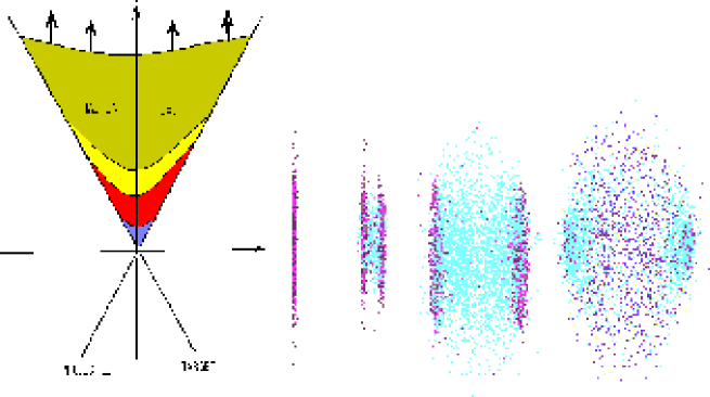
Figure 1: Schematic space–time view of a heavy ion collision that indicates four basic stages in the evolution of the collision fireball: initial overlap region, pre–equilibrium partonic system, equilibrated quark-gluon plasma and its subsequent hadronization to a hadron gas.

Both of these pieces of information can be obtained today from first principle calculations by formulating QCD on the lattice and performing Monte-Carlo simulations. In Fig. (2) we show the most recent results[77] of lattice gauge theory (LGT) for the temperature dependence of energy density and pressure. These results have been obtained in LGT for different numbers of dynamical fermions. The energy density is seen in Fig. (2) to exhibit the typical behavior of a system with a phase transition: an abrupt change in a very narrow temperature range. The corresponding pressure curve shows a smooth change with temperature. In the region below $T_{c}$ the basic constituents of QCD, quarks and gluons, are confined within hadrons and here the EoS is well parameterized[79] by a hadron resonance gas. Above $T_{c}$ the system appears in the QGP phase where quarks and gluons can travel distances that substantially exceed the typical size of hadrons. The most recent results of improved perturbative expansion of the thermodynamical potential in continuum QCD indicate[81, 83] that, at some distance above $T_{c}$, the EoS of QGP can be well described by a gas of massive quasi-particles with a temperature dependent mass. In the vicinity of $T_{c}$ the relevant degrees of freedom were argued[84, 85] to be described by Polyakov loops.

Lattice Gauge Theory predicts, in two–flavour QCD, a critical temperature $T_{c}=173\pm~{}8$MeV and corresponding critical energy density $\epsilon_{c}=0.6\pm 0.3$ GeV/fm³ for the deconfinement phase transition[77]. The value of $\epsilon_{c}$ is surprisingly low and corresponds quantitatively to the energy density inside the nucleon.

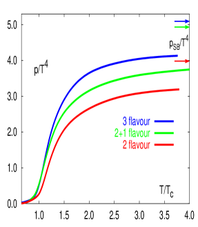
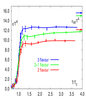
Figure 2: The pressure $P$ and energy density $\epsilon$ normalized to the temperature to the fourth power, versus temperature normalized to its critical value. The calculations[77] were performed within LGT for different numbers of flavors. The values of the corresponding ideal gas results are indicated by the arrows.

The initial energy density reached in heavy ion collisions can be estimated within the Bjorken model[78]. From the transverse energy $E_{T}$ measured in nucleus–nucleus collisions the initial energy density $\epsilon_{0}$ is determined as

$$\epsilon_{0}(\tau_{0})={1\over{\pi R^{2}}}{1\over\tau_{0}}{{dE_{T}}\over{dy}},$$ (1)

where the initially produced collision fireball is considered as a cylinder of length $dz=\tau_{0}dy$ and transverse radius $R\sim A^{1/3}$. Inserting for $\pi R^{2}$ the overlap area of colliding Pb nuclei together with an assumed initial time of $\tau_{0}\simeq 1$ fm, and using an average transverse energy at midrapidity measured[86] at the SPS ($\sqrt{s}=17.3$ GeV) to be 400 GeV, one obtains

$$\epsilon_{0}^{SPS}(\tau_{0}\simeq 1~{}{\rm fm})\simeq 3.5\pm 0.5~{}{\rm GeV/{\rm fm}^{3}}.$$ (2)

Increasing the collision energy to $\sqrt{s}=130$ A$\cdot$GeV for Au–Au at RHIC and keeping the same initial thermalization time as at the SPS, would increase $\epsilon_{0}$ by only 50–60 $\%$. However, at RHIC the thermalization time was argued in terms of different models[10, 90] to be shorter by a factor of 3–5.

In the context of saturation models[10, 87]^-[89] the thermalization time can be possibly related with the saturation scale[8, 10]. The basic concept of the saturation models is the conjecture that there is some transverse momentum scale $p_{\rm sat}$ where the gluon and quark phase space density saturates[10, 87]^-[89]. For an isentropic expansion of the collision fireball, the transverse energy at $p_{\rm sat}$ was related in Ref. (r28) to that measured in nucleus–nucleus collisions in the final state. The saturation scale was also used to fix the thermalization time as $\tau_{eq}\simeq 1/p_{\rm sat}$. Taking the value of $p_{\rm sat}$ predicted in Ref. (r28) for RHIC energy, $p_{\rm sat}\simeq 1.13$ GeV, one gets $\tau_{eq}\simeq 0.2$ fm and a corresponding energy density $\epsilon_{eq}\simeq 98$ GeV/fm³. This is a larger value than expected for the initial energy density at RHIC in the McLerran–Venugopalan model[88] where $\epsilon_{0}^{RHIC}\sim 20$ GeV/fm³, also in agreement with the prediction of Ref. (r30).

At SPS energy the saturation model described in Ref. (r28) leads to $\epsilon_{eq}^{SPS}\sim 16$ GeV/fm³, a much higher value than that obtained from Eq. (2). The estimate of $\epsilon_{eq}$ and initial thermalization time strongly depends on the value of $p_{\rm sat}$ and the model assumptions. In a $"$ bottom–up $"$ equilibration scenario[8] the thermalization time in Au–Au collisions at RHIC energy was estimated to be as large as 3.2–3.6 fm and the temperature $T\simeq$(210–230) MeV. Nevertheless, this initial temperature still corresponds to an energy density by factor of 2–3 larger then that required for deconfinement. In A–A collisions at the LHC the initial energy density of the equilibrated partonic medium is expected[10, 92] to be in the range $400<\epsilon_{eq}^{LHC}<1300$ GeV/fm³.

The dominant constituents of the partonic medium produced in ultrarelativistic heavy ion collisions at LHC, RHIC and even at SPS energy are gluons. The energy density of gluons in thermal equilibrium scales with the fourth power of the temperature $\epsilon=gT^{4}$, where $g$ is related to the number of degrees of freedom. For an ideal gluon gas, $g=16\pi^{2}/30$; in an interacting system, the effective number of degrees of freedom $g$ is smaller. The results of LGT shown in Fig. 2 indicate deviations from the Boltzmann limit by 20–25 $\%$. Relating the thermal energy density with the initial energy density discussed above, one can make an estimate of the initial temperature reached in heavy ion collisions. For the SPS, RHIC and LHC energies this gives a temperature in the range: $200~{}{\rm MeV}<T^{SPS}<330$ MeV, $210~{}{\rm MeV}<T^{RHIC}<600$ MeV and $1000~{}{\rm MeV}<T^{LHC}<1200$ MeV, respectively.

Comparing the initial energy density expected in heavy ion collisions with LGT results, it is clear, that the initial energy density at LHC and RHIC by far exceeds the critical value. A large energy density is, however, still not sufficient to create a QGP. The distribution of initially produced gluons is very far from being thermal, thus the system needs enough time to equilibrate. Recently it was shown[8], in the framework of perturbative QCD and kinetic theory, that the equilibration of partons should definitely happen at LHC and most likely at RHIC energy.

A previous microscopic study[93] within the Parton Cascade Model has led to the conclusion that thermalization can also be reached even at the lower SPS energy. Here, however, due to the relatively low collision energy, it is not clear whether a model inspired by perturbative QCD is indeed applicable.

Assuming QGP formation in the initial state in heavy ion collisions one expects that the thermal nature of the partonic medium could be preserved during hadronization. Consequently, the particle yields measured in the final state should resemble a thermal equilibrium population.

2 Statistical approach - general remarks

In the approach of Gibbs (see, e.g., Ref. (huang)) the equilibrium behavior of thermodynamical observables can be evaluated as an average over statistical ensembles (rather than as a time average for a particular state). The equilibrium distribution is thus obtained by an average over all accessible phase space. Furthermore, the ensemble corresponding to thermodynamic equilibrium is that for which the phase space density is uniform over the accessible phase space. In this sense, filling the accessible phase space uniformly is both a necessary and sufficient condition for equilibrium. Consequently, the agreement between observables and predictions using the statistical operator imply equilibrium (to the accuracy with which agreement is observed). ”Filling phase space” is not a different statement, although it is often and erroneously used in the literature.

In our further analysis we use in the statistical operator as Hamiltonian that leading to the full hadronic mass spectrum. In some sense this is synonymous with using the full QCD Hamiltonian. The only parameters in the statistical operator describing the grand-canonical ensemble are temperature $T$ and baryon chemical potential $\mu_{B}$. There is no room here for strangeness suppression ($\gamma_{s}$) factors. So the interpretation is that agreement between data and theoretical predictions implies statistical equilibrium at temperature T and chemical potential $\mu_{B}$. If an additional factor $\gamma_{s}$ is needed to describe the data this implies a clear deviation from chemical equilibrium: a state in which e.g. strangeness is suppressed compared to the equilibrium value implies additional dynamics not contained in the statistical operator and not consistent with uniform phase space density. Similar arguments, of course, apply if one uses canonical phase space. If, in this regime, canonically calculated particle ratios agree with those measured, this implies equilibrium at temperature $T$ and over the canonical volume $V$. To the extent that this describes data for e+e- or pp collisions, the same conclusions on thermodynamic equilibrium apply. However, we note that, in this approach e.g., particles ratios involving particles with hidden strangeness are generally not well predicted, again implying non-equilibrium behavior.

2.1 Statistical approach - grand canonical formalism

The basic quantity required to compute the thermal composition of particle yields measured in heavy ion collisions is the partition function $Z(T,V)$. In the Grand Canonical (GC) ensemble,

$$Z^{GC}(T,V,\mu_{Q})={\rm Tr}[e^{-\beta(H-\sum_{i}\mu_{Q_{i}}Q_{i})}],$$ (3)

where $H$ is the Hamiltonian of the system, $Q_{i}$ are the conserved charges and $\mu_{Q_{i}}$ are the chemical potentials that guarantee that the charges $Q_{i}$ are conserved on the average in the whole system. Finally $\beta=1/T$ is the inverse temperature. The Hamiltonian is usually taken such as to describe a hadron resonance gas. For practical reasons, the hadron mass spectrum contains contributions from all mesons with masses below $\sim$1.5 GeV and baryons with masses below $\sim$2 GeV. In this mass range the hadronic spectrum is well established and the decay properties of resonances are reasonably well known[91]. This mass cut in the contribution of resonances to the partition function limits, however, the maximal temperature to $T_{\rm max}\simeq 200$ MeV, up to which the model predictions may be considered trustworthy[37, 38, 42, 58]. For higher temperatures the contributions of ( in general poorly known) heavier resonances are not negligible. The interaction of hadrons and resonances are usually only included by implementing a hard core repulsions, i.e. a Van der Waals–type interaction. Details of such a implementation are discussed below. The main motivation of using the Hamiltonian of a hadron resonance gas in the partition function is that it contains all relevant degrees off freedom of the confined, strongly interacting medium and implicitly includes interactions that result in resonance formation. Secondly, this model is consistent with the equation of state obtained from the LGT below the critical temperature[79, 80]. In a strongly interacting medium, one includes the conservation of electric charge, baryon number and strangeness. The GC partition function (3) of a hadron resonance gas can then be written as a sum of partition functions $\ln Z_{i}$ of all hadrons and resonances

$$\ln Z(T,V,\vec{\mu})=\sum_{i}\ln Z_{i}(T,V,\vec{\mu}),$$ (4)

where $\epsilon_{i}=\sqrt{p^{2}+m_{i}^{2}}$ and $\vec{\mu}=(\mu_{B},\mu_{S},\mu_{Q})$ with the chemical potentials $\mu_{i}$ related to baryon number, strangeness and electric charge, respectively. For particle $i$ of strangeness $S_{i}$, baryon number $B_{i}$, electric charge $Q_{i}$ and spin–isospin degeneracy factor $g_{i}$,[2]

$$\ln Z_{i}(T,V,\vec{\mu})={{Vg_{i}}\over{2\pi^{2}}}\int_{0}^{\infty}\pm p^{2}dp\ln[1\pm\lambda_{i}\exp(-\beta\epsilon_{i})],$$ (5)

with (+) for fermions, (-) for bosons and fugacity

$$\lambda_{i}(T,\vec{\mu})=\exp({{B_{i}\mu_{B}+S_{i}\mu_{S}+Q_{i}\mu_{Q}}\over T})$$ (6)

Expanding the logarithm and performing the momentum integration in Eq. (5) we obtain

$$\ln Z_{i}(T,V,\vec{\mu})={{VTg_{i}}\over{2\pi^{2}}}\sum_{k=1}^{\infty}{{(\pm 1)^{k+1}}\over{k^{2}}}\lambda_{i}^{k}m_{i}^{2}K_{2}({{km_{i}}\over T}),$$ (7)

where $K_{2}$ is the modified Bessel function and the upper sign is for bosons and lower for fermions. The first term in Eq. (7) corresponds to the Boltzmann approximation. The density of particle $i$ is obtained from Eq. (7) as

$$n_{i}(T,\vec{\mu})={{{\langle N_{i}\rangle}\over V}}={{Tg_{i}}\over{2\pi^{2}}}\sum_{k=1}^{\infty}{{(\pm 1)^{k+1}}\over{k}}\lambda_{i}^{k}m_{i}^{2}K_{2}({{km_{i}}\over T}),$$ (8)

Figure 3: The ratio of the total density of positively charged pions that includes all resonance contributions to the density of thermal pions. The calculations are done in the hadron resonance gas model for $\mu_{B}=$250, 550 MeV and for different temperatures.

The partition function (4) is the basic quantity that allows to describe all thermodynamical properties of a fireball composed of hadrons and resonances being in thermal and chemical equilibrium. In view of further application of this statistical operator to the description of particle production in heavy ion collisions we write explicitly the results for particle density obtained from Eq. (4). Of particular importance here is to account for resonances and their decay into lighter particles. The average number $\langle N_{i}\rangle$ of particles $i$ in volume $V$ and temperature $T$, that carries strangeness $S_{i}$, baryon number $B_{i}$, and electric charge $Q_{i}$, is obtained from Eq. (4) as

$$\langle N_{i}\rangle(T,\vec{\mu})~{}=~{}\langle N_{i}\rangle^{th}(T,\vec{\mu})+{\sum}_{j}\Gamma_{j\to i}\langle N_{j}\rangle^{th,R}(T,\vec{\mu})$$ (9)

where the first term describes the thermal average number of particles of species $i$ and second term describes overall resonance contributions to particle multiplicity of species $i$. This term is taken as a sum of all resonances that decay into particle $i$. The $\Gamma_{j\to i}$ is the corresponding decay branching ratio of $j\to i$. The corresponding multiplicities in Eq. (9) are obtained from Eq. (8). The importance of the resonance contribution to the total particle yield in Eq. (9) is illustrated in Fig. (3) as the ratio of total to thermal number of $\pi^{+}$. From this figure it is clear that at high temperature (or density) the overall multiplicity of light hadrons is indeed dominated by resonance decays. In the high-density regime, that is for large $T$ and/or $\mu_{B}$, the repulsive interactions of hadrons should be included in the partition function (4). To incorporate the repulsion at short distances one usually uses a hard core description by implementing excluded volume corrections[58]. In a thermodynamically consistent approach[82] these corrections lead to a shift of the baryon–chemical potential. . We discuss below how this is implemented in our calculations. The repulsive interactions are important when discussing observables of density type. Particle density ratios, however, are only weakly affected[38] by the repulsive corrections. The partition function (4) depends in general on five parameters. However, only three are independent, since the isospin asymmetry in the initial state fixes the charge chemical potential and the strangeness neutrality condition eliminates the strange chemical potential. Thus, on the level of particle multiplicity ratios we are only left with temperature $T$ and baryon chemical potential $\mu_{B}$ as independent parameters. In Fig. (4) we show the relation of $\mu_{S}=\mu_{S}(T,\mu_{B})$ obtained from the strangeness neutrality condition. For low temperature this relation is highly non-linear. For larger $T$, however, $\mu_{S}$ shows an almost linear dependence on $\mu_{B}$. One sees by inspection of Fig. (4) that, at $T\sim 200$ MeV and $\mu_{B}\sim 300$ MeV, $\mu_{S}\sim{1\over 3}\mu_{B}$. This relation is obtained in a QGP from strangeness neutrality conditions. In the present context of a hadron resonance gas this is a pure accident with no dynamical information.

Figure 4: The strange chemical potential $\mu_{S}$ as a function of baryon–chemical potential for T=120,170 and 200 MeV. The results are obtained by imposing the strangeness neutrality condition in a hadron resonance gas.

At lower energies, in practise for $T<100$ MeV, the widths of the resonances have to be included[49, 25] in Eq. (9). This is because the number of light particles coming from the decay of resonances is increased by the finite resonance width. In practice, the width of the $\Delta$ resonance is most important[25, 27]. Thus, the approximation of the resonance width by a $\delta$ function is not justified. Assuming the validity of Boltzmann statistics one replaces the partition function in equation (7) by:

$$\ln Z_{R} = N\,{{Vd_{R}}\over{2\pi^{2}}}\,T\,\exp[(B_{R}\mu_{B}+Q_{R}\mu_{Q}+S_{R}\mu_{S})/T]\,$$ (10)

$$\int_{s_{min}}^{s_{max}}ds\,s\,K_{2}(\sqrt{s}/T)\,{1\over\pi}\,{{m_{R}\Gamma_{R}}\over{(s-m_{R}^{2})^{2}+m_{R}^{2}\Gamma_{R}^{2}}}$$

where $s_{min}$ is chosen to be the threshold value for the resonance decay and $\sqrt{s_{max}}\sim m_{R}+2\Gamma_{R}$. The normalization constant $N$ is adjusted such that the integral over the Breit-Wigner factor gives 1.

The statistical model, outlined above, was applied[34]^-[75, 76] to describe particle yields in heavy ion collisions. The model was compared with all available experimental data obtained in the energy range from AGS up to RHIC energy. Hadron multiplicities ranging from pions to omega baryons and their ratios were used to verify that there is a set of thermal parameters $(T,\mu_{B})$ which simultaneously reproduces all measured yields. In the following Section we present the most recent analysis of particle production in A–A collisions at RHIC, SPS and AGS energies.

2.2 Thermal analysis of particle yields from AGS to RHIC energies

For the analysis of data in the energy range of 40 GeV/nucleon and upwards we use a grand canonical ensemble to describe the partition function and hence the density of the particles following Eqs. (4 -9). As discussed above the temperature $T$ and the baryochemical potential $\mu_{B}$ are the two independent parameters of the model, while the volume of the fireball $V$, the strangeness chemical potential $\mu_{S}$, and the charge chemical potential $\mu_{Q}$ are fixed by the following additional conditions. First, overall strangeness conservation fixes $\mu_{S}$. Note that this applies strictly for data integrated over 4$\pi$. For slices near mid-rapidity this condition is, however, also appropriate as the flow of strangeness in and out of the rapidity slice under consideration very nearly cancels. Charge conservation implies a condition on $I^{3}$ according to:

$$V\sum_{i}n_{i}I^{3}_{i}=\frac{Z-N}{2}.$$ (11)

Here, Z and N are the proton and neutron numbers of the colliding nuclei, $I^{3}$ and $I^{3}_{i}$ are the third component of the total isospin and that of particle i. This condition is appropriate (and relevant) at lower beam energies where there is full stopping and 4$\pi$ yields are used. For details see Refs. (r12,diplomarbeit). At higher energies and for data analyzed in rapidity slices the right hand side of Eq. ( 11) has to be replaced by the neutron excess of baryons transported into the rapidity slice under consideration. This number is clearly smaller than the full neutron excess entering Eq.  (11) but in general not well known. However, its precise knowledge is less relevant for higher beam energies since the isospin balance is dominated by pions. For practical purposes isospin conservation is important for AGS energies and below but its effect is small (on the 10 % level) already at 40 GeV/nucleon beam energy (where we have used as an upper limit the full neutron excess of the colliding nuclei, leading to a slight overestimate of the pion charge asymmetry) and negligible at top SPS and RHIC energies. Finally, the volume (which drops out anyway for particle ratios) can be obtained from total baryon number conservation (for full stopping and quantities which are evaluated over the complete phase space) or is fixed by using the measured pion multiplicity in the rapidity slice under consideration. As discussed above the hadronic mass spectrum used in the calculations extends over all mesons with masses below 1.5 GeV and baryons with masses below 2 GeV. To take into account a more realistic equation of state we incorporate the repulsive interaction at short distances between hadrons by means of the excluded volume correction discussed above. A number of different corrections have been discussed in the literature. Here we choose that proposed in Refs. (diplomarbeit,exclv2,r79):

$$p^{excl.}(T,\mu)=p^{id.gas}(T,\hat{\mu});\quad\mbox{with }\hat{\mu}=\mu-v_{eigen}\;p^{excl.}(T,\mu).$$ (12)

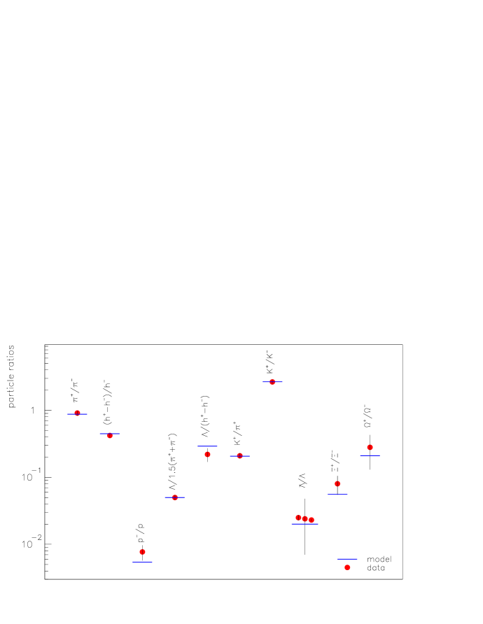
Figure 5: Comparison between thermal model predictions and experimental particle ratios for Pb–Pb collisions at 40 GeV/nucleon. The thermal model calculations are obtained with $T=148$ MeV and $\mu_{B}=400$ MeV.

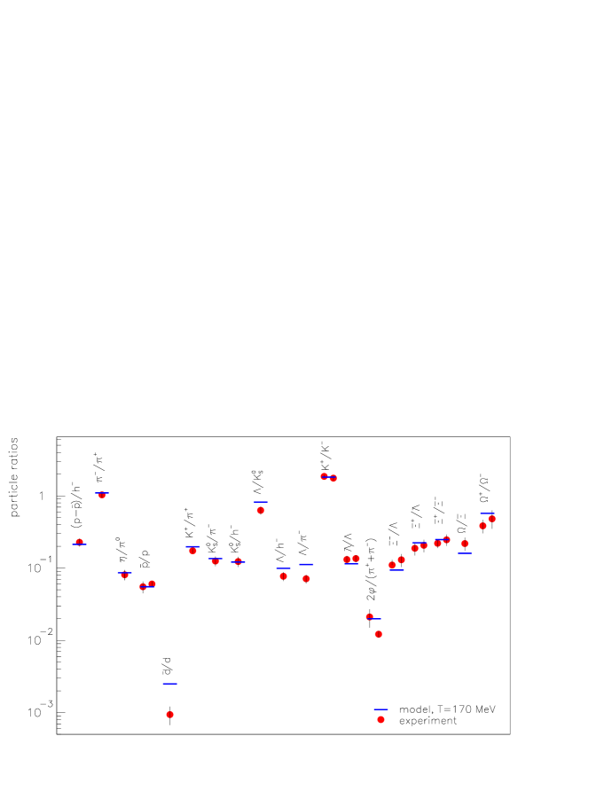
Figure 6: Comparison between thermal model predictions and experimental particle ratios for Pb–Pb collisions at 158 GeV/nucleon. The thermal model calculations are obtained with $T=170$ MeV and $\mu_{B}=255$ MeV.

This thermodynamically consistent approach to simulate interactions between particles by assigning an eigenvolume $v_{eigen}$ to all particles modifies the pressure $p$ within the fireball. Equation (12) is recursive, as it uses the modified chemical potential $\hat{\mu}$ to calculate the pressure, while this pressure is also used in the modified chemical potential, and the final value is found by iteration. Particle densities are calculated by substituting $\mu$ in Eq.  (8) by the modified chemical potential $\hat{\mu}$. The eigenvolume has to be chosen appropriately to simulate the repulsive interactions between hadrons, and we have investigated the consequences for a wide range of parameters for this eigenvolume in Ref. (r12,diplomarbeit). Note that the eigenvolume is $v_{eigen}=4\frac{4}{3}\pi R^{3}$ for a hadron with radius R. Assigning the same eigenvolume to all particles can reduce particle densities drastically but hardly influences particle ratios. Ratios may differ strongly, however, if different values for the eigenvolume are used for different particle species. Our approach here is, to determine, for nucleons, the eigenvolume according to the hard-core volume known from nucleon-nucleon scattering[62]. Consequently, we assigned 0.3 fm as radius for all baryons. For mesons we expect the eigenvolume not to exceed that of baryons. For lack of better theoretical guidance we chose also for the mesons a radius of 0.3 fm. For a discussion of the implications of varying these radius parameters see Ref. (r12,diplomarbeit). After thermal “production”, resonances and heavier particles are allowed to decay, therefore contributing to the final particle yield of lighter mesons and baryons, as indicated above. Decay cascades, where particles decay in several steps, are also included. Systematic parameters regulate the amount of decay products resulting from weak decays. This allows to simulate the different reconstruction efficiencies for particles from weak decays in different experiments. In the following we compare predictions of the model with results of measured particle ratios for central Pb-Pb collisions at SPS energies (40 and 158 GeV/nucleon) and for central Au-Au collisions at RHIC energies $\sqrt{s_{nn}}=$ 130 and 200 GeV. An important issue in this context is whether to use data at mid-rapidity or data integrated over the full phase space. While it is clear that full 4$\pi$ yields should be used at low beam energies, this is not appropriate any more as soon as fragmentation and central regions can be distinguished. In that case the aim is to identify a boost-invariant region near mid-rapidity and to choose a slice in rapidity within that region. For RHIC energies this implies that an appropriate choice, given the available data, is a rapidity interval of width $\Delta y=1$ centered at midrapidity. The anti-proton/proton ratio stays essentially constant within that interval, but drops rather strongly for larger rapidities and similar results are observed[63] for other ratios. Furthermore, the rapidity distribution exhibits a boost-invariant plateau near mid-rapidity[64]. As has been demonstrated in Ref. (cleymans), effects of hydrodynamic flow cancel out in particle ratios under such conditions. At SPS energies a boost-invariant plateau is not fully developed but stopping is not complete, either. In addition, the proton and anti-proton rapidity distributions differ rather drastically, especially near the fragmentation regions, implying that particle ratios depend on rapidity (see. e.g., Ref. (appels1)). Under those circumstances we have decided to use, wherever available, data in a slice of $\pm 1$ unit of rapidity centered at mid-rapidity. This is slightly different from the analysis performed in Ref. (r12), where both mid-rapidity and fully integrated data were used. We note, however, see below, that the fit parameters T and $\mu_{B}$ obtained at 158 A GeV are very close to those determined earlier. The criterion for the best fit of the model to data was a minimum in

$$\chi^{2}=\sum_{i}\frac{({\cal R}_{i}^{\rm exp.}-{\cal R}_{i}^{\rm model})^{2}}{\sigma_{i}^{\rm 2}}.$$ (13)

In the above equations ${\cal R}_{i}^{\rm model}$ and ${\cal R}_{i}^{\rm exp.}$ are the $i$th particle ratio as calculated from our model or measured in the experiment, and $\sigma_{i}$ represent the errors (including systematic errors where available) in the experimental data points as quoted in the experimental publications. For the data we used all information available including that presented at the QM2002 conference in July 2002. Details on the data selection, corrections for the weak-decay reconstruction efficiency, as well relevant references are found in Ref. (magestro3). Under the conditions discussed above the data can all be well described, as is detailed below, by a thermal distribution with T and $\mu_{B}$ as independent parameters. There is no need to introduce additional parameters such as as strangeness suppression factors.

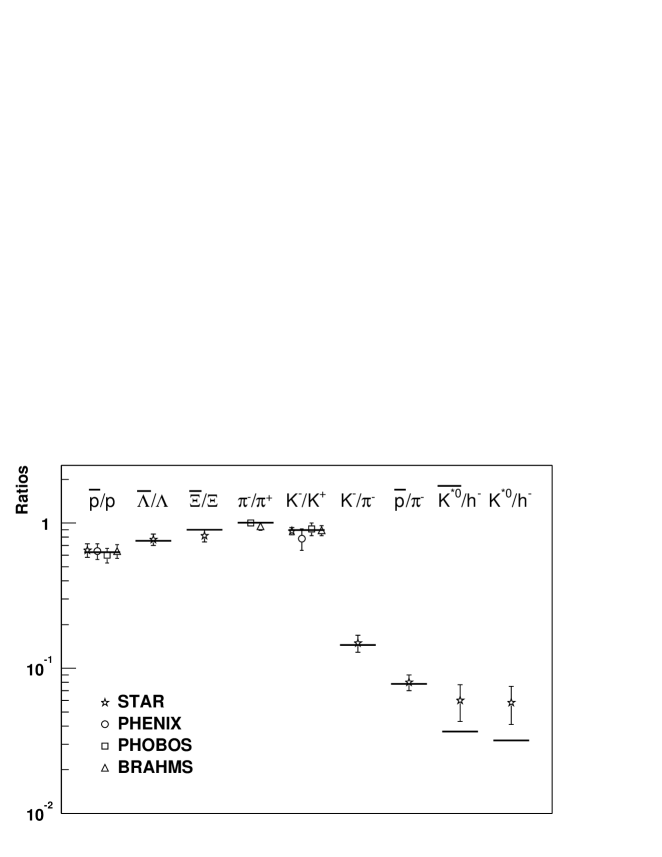
Figure 7: Comparison between thermal model predictions[35] and experimental particle ratios for Pb–Pb collisions at $\sqrt{s_{nn}}$ = 130 GeV. Calculations were performed for $T=174$ MeV and $\mu_{B}$ = 46 MeV.

The results of the fits for central Pb-Pb collisions at 40 and 158 GeV per nucleon are presented in Figs. (5,6). At 40 GeV/nucleon 11 particle ratios are included in the fit, while the number is 24 at 158 GeV/nucleon. We obtain values for (T,$\mu_{B}$) of (148$\pm 5$, 400$\pm 10$) and (170$\pm 5$, 255$\pm 10$), respectively, with reduced $\chi^{2}$ values of 1.1 and 2.0. Obviously the fits are quite good. A possible exception is the $\phi/(\pi^{+}+\pi^{-})$ ratio at top SPS energy, where there are conflicting data from NA49 and NA50. This is already discussed in detail in Ref. (r12) and no new information on this problem has appeared since. Note that this ratio has not been used in the $\chi^{2}$ minimization. The somewhat larger values of $\chi^{2}$ at full SPS energy and the remaining uncertainty in $\mu_{B}$ are due to a systematic problem not yet sufficiently addressed by the experiments. The contribution of weak decays of strange baryons to final baryons has been discussed and cuts are applied to reduce this contribution in the data. However, there is also a contribution from weak decays to charged pions (or, more generally) charged hadrons which is up to now poorly quantified by the experiments. If, e.g., in the ratio $\Lambda/h^{-}$, feeding of the $\Lambda$ by decays of $\Xi$’s is suppressed due to cuts, but the $\pi^{-}$ measurement has a 50 % efficiency for detection of pions from weak decays, the ratio would drop by 15-20 %, compared to the case with 0 % eficiency for weak decays. With this option the reduced $\chi^{2}$ value for the 158 GeV fit would drop from 2.0 to 1.5. This discussion indicates that there are sources of systematic uncertainties not included in the data. The corrections for weak decays are, consequently, of utmost importance when discussing the “precision” of fits.

Figure 8: Comparison of the experimental data on different particle multiplicity ratios obtained at RHIC at $\sqrt{s}_{NN}=130$ and 200 GeV with thermal model calculations. The thermal model analysis is from Refs. (r10,r10n) and recent update by D. Magestro.

The results for RHIC energies are shown in Figs. (7, 8). In Fig. (7) we present the results as published in Ref. (r10) in the summer of 2001. Since then, the data at $\sqrt{s_{nn}}=130$ GeV have been consolidated and extended and first (in some cases still preliminary) results have been provided for $\sqrt{s_{nn}}=200$ GeV. The current state of affairs in summarized in Fig. (7). The results demonstrate quantitatively the high degree of equilibration achieved for hadron production in central Au-Au collisions at RHIC energies. We obtain values for (T,$\mu_{B}$) of (174$\pm 7$, 46$\pm 5$) and (177$\pm 7$, 29$\pm 6$), respectively, with reduced $\chi^{2}$ values of 0.8 and 1.1. We note that ratios involving multi-strange baryons are well reproduced as is the $\phi/h^{-}$ ratio. Even relatively wide resonances such as the K^∗’s fit well into the picture of chemical freeze-out. This obviates the need for quark coalescence models as proposed in Ref. (biro1) and non-equilibrium models as proposed in Ref. (rafelski).

Very recently, the STAR collaboration has provided[69] first data, with about 30 - 50 % accuracy, on the $\rho^{0}/\pi$ and $f^{0}(980)/\pi$ ratios in semi-central Au-Au collisions. These mesons have been reconstructed in STAR via their decay channel in 2 charged pions. Comparing the preliminary results from STAR with our thermal model prediction reveals that the measured ratios exceed the calculated values by about a factor of 2. This is quite surprising, especially considering that we use a chemical freeze-out temperature of 177 MeV for the calculation, while one might expect these wide resonances to be formed near to thermal freeze-out, i.e. at a temperature of about 120 MeV. At this temperature, the equilibrium value for the $\rho^{0}/\pi$ ratio is about $4\cdot 10^{-4}$, while it is 0.11 at 177 MeV. Even with a chemical potential for pions of close to the pion mass and taking into account the apparent (downwards) mass shift of 60 - 70 MeV for the $\rho^{0}$ it seems difficult to explain the experimentally observed value of about 0.2.

We finally note that the model discussed here was also applied to the AGS data collected in Ref. (r11). The best fit, obtained for R_baryon=R_meson=0.3 fm, yields T = 125 (+3-6) MeV and $\mu_{B}$ = 540 $\pm 7$ MeV, well in line with the calculations reported in Ref. (r11).

In summary, hadron multiplicities produced in central nucleus-nucleus collisions in the range of AGS to full RHIC energy can be quantitatively described with a grand-canonical partition function based on the full hadron resonance spectrum, assuming complete chemical equilibrium. There is no need to introduce non-equilibrium parameters or strangeness suppression factors if data near mid-rapidity are considered. The physical relevance of the two model parameters T and $\mu_{B}$ is described in detail in our discussions below concerning the phase boundary between hadrons and the quark-gluon plasma.

2.3 Comparison of measured particle densities with thermal model predictions

As discussed below, the value for the energy density predicted by the presently used thermal model, including the excluded volume correction, agrees well with results from the lattice for temperatures below the critical temperature. It makes therefore sense to compare the densities for pions and nucleons predicted by the model with values determined from experiments. The CERES collaboration has recently performed an analysis of 2-pion correlation experiments for the energy range between AGS and RHIC, from which values for these densities have been determined[70, 71] from data taken at mid-rapidity. For the nucleon density (at thermal freeze-out) the experimental numbers are, at 40 and 158 GeV/nucleon and at $\sqrt{s_{nn}}=130$ GeV, 0.077 $\pm 0.005$/fm³, 0.063 $\pm 0.005$/fm³ and 0.06 $\pm 0.009$/fm³. From the model we deduce, at chemical freeze-out, values of 0.10/fm³, 0.10/fm³ and 0.08/fm³. This would imply a volume increase of about 40 % from chemical to thermal freeze-out. For pions the situation could be more complicated since yield ratios involving pions are (apparently) fixed at chemical freeze-out, implying the build-up of a pion chemical potential between chemical and thermal freeze-out. From the data one deduces[70, 71] a pion density at (thermal) freeze-out of 0.28 $\pm 0.03$/fm³, 0.43 $\pm 0.03$/fm³, and 0.49 $\pm 0.1$/fm³, at 40 and 158 GeV/nucleon and at $\sqrt{s_{nn}}=130$ GeV. These values should be contrasted with the calculated (chemical) freeze-out values of 0.35/fm³, 0.59/fm³ and 0.62/fm³. From these numbers one would conclude a 30 % volume increase between chemical and thermal freeze-out, assuming that the pion chemical potential fixes the pion number to the value obtained at chemical freeze-out. This rather small volume increase indicates that the time between chemical and thermal freeze-out cannot be very long at SPS and RHIC energies. At AGS energy, the corresponding $\pi^{+}$ and proton densities of 0.051/fm³ and 0.053/fm³ agree well with those estimated[73, 74] from particle interferometry (0.058/fm³ and 0.063/fm³, respectively) implying that, at AGS energy, thermal and chemical freeze-out take place at nearly identical times and temperatures.

2.4 Statistical model and composite particles

An often overlooked aspect of the thermal model is the possibility to compute also the yields of composite particles. For example, the d/p and $\bar{\rm{d}}/\bar{\rm{p}}$ ratios measured at SPS and AGS energies are well reproduced[97] with the same parameters which are used to describe[37, 38] baryon and meson ratios. Furthermore, the AGS E864 Collaboration has recently published[95] yields for composite particles (light nuclei up to mass number 7) produced in central Au-Au collisions at AGS energy near mid-rapidity and at small $p_{t}$. In this investigation, an exponential decrease of composite particle yield with mass is observed over 7–8 order of magnitude, yielding a penalty factor $P_{p}$ of about 48 for each additional nucleon. Extrapolation of the data to large transverse momentum values, considering the observed mass dependence of the slope constants, reduces this penalty factor to about 26, principally because of transverse flow. In the thermal model, this penalty factor can be related with thermal particle phase–space. In the relevant Boltzmann approximation, we obtain

$$R_{p}\approx\exp{\frac{m\pm\mu_{b}}{T}},$$ (14)

where m is the nucleon mass and the negative sign applies for matter, the positive for anti-matter. Small corrections due to the spin degeneracy and the A^3/2 term in front of the exponential in the Boltzmann formula for particle density are neglected. Using the freeze–out parameters T=125 MeV and $\mu_{b}=$ 540 MeV appropriate[37] for AGS energy one gets[97] R${}_{p}\approx 23$, in close agreement with the data for the production of light nuclei. It was also noted that the anti-matter yields measured[96] by the E864 Collaboration yield penalty factors of about 2$\cdot 10^{5}$, again close to the predicted[97] value of 1.3$\cdot 10^{5}$ .

This rather satisfactory quantitative agreement between measured relative yields for composite particles and thermal model predictions provides some confidence in the predictions for yields of exotic objects produced in central nuclear collisions. We briefly comment here on the results obtained in Ref. (col3).

In this investigation, the production probabilities for exotic strange objects and, in particular, for strangelets were computed in the thermal model. The results are reproduced in Table 2.4 for temperatures relevant for beam energies between 10 and 40 GeV/nucleon. We first note that predictions of the thermal model and, where available, the coalescence model of Ref. (col4) agree (maybe surprisingly) well particularly for lighter clusters. Secondly, inspection of Table 2.4 also shows that, in future high statistics experiments which will be possible at the planned[180] new GSI facility, multi-strange objects such as ${}_{\Xi^{0}\Lambda\Lambda}^{~{}~{}~{}~{}~{}7}$He should be experimentally accessible with a planned sensitivity of about 10^-13 per central collision in a years running, should they exist and be produced with thermal yields. Investigation of yields of even the lightest conceivable strangelets will be difficult, though.

Produced number of nonstrange and strange clusters and of strange quark matter per central Au+Au collision at AGS energy, calculated in a thermal model for two different temperatures, baryon chemical potential $\mu_{b}$= 0.54 GeV and strangeness chemical potential $\mu_{s}$ such that overall strangeness is conserved.             Thermal Model Parameters Particles $T$=0.120 GeV $T$=0.140 GeV Coalescence d 15 19 11.7 t+³He 1.5 3.0 0.8 $\alpha$ 0.02 0.067 0.018 $H_{0}$ 0.09 0.15 0.07 ${}_{\Lambda\Lambda}^{~{}~{}~{}5}$H 3.5 $\cdot 10^{-5}$ 2.3 $\cdot 10^{-4}$ 4$\cdot 10^{-4}$ ${}_{\Lambda\Lambda}^{~{}~{}~{}6}$He 7.2 $\cdot 10^{-7}$ 7.6 $\cdot 10^{-6}$ 1.6$\cdot 10^{-5}$ ${}_{\Xi^{0}\Lambda\Lambda}^{~{}~{}~{}~{}~{}7}$He 4.0 $\cdot 10^{-10}$ 9.6 $\cdot 10^{-9}$ 4 $\cdot 10^{-8}$ ${}^{10}_{1}$St^-8 1.6 $\cdot 10^{-14}$ 7.3 $\cdot 10^{-13}$ ${}^{12}_{1}$St^-9 1.6 $\cdot 10^{-17}$ 1.7 $\cdot 10^{-15}$ ${}^{14}_{1}$St^-11 6.2 $\cdot 10^{-21}$ 1.4 $\cdot 10^{-18}$ ${}^{16}_{2}$St^-13 2.4 $\cdot 10^{-24}$ 1.2 $\cdot 10^{-21}$ ${}^{20}_{2}$St^-16 9.6 $\cdot 10^{-31}$ 2.3 $\cdot 10^{-27}$ [Source] The Coalescence model predictions in the last column are from Table 2 of Ref. (col4).

3 Exact Implementation of the conservation laws in the statistical models

The analysis of particle yields obtained in central heavy ion collisions from AGS up to LHC energy has shown that hadron multiplicities are very well described by assuming a complete thermalized state at fixed $T$ and $\mu_{B}$ . In this broad energy range, particle yields and their ratios are, within experimental error, well reproduced by the statistical hadron resonance gas model that accounts for the conservation laws of baryon number, strangeness and electric charge in the grand canonical ensemble. The natural question arising here is whether this statistical order is a unique feature of high energy central heavy ion collisions or is it also there at lower energies as well as in hadron–hadron and peripheral heavy ion collisions. To address this question one needs, however, to stress that when going beyond high energy central heavy ion collisions the grand canonical statistical operator (3) has to be modified.

Within the statistical approach, particle production can only be described using the grand canonical ensemble with respect to conservation laws, if the number of produced particles that carry a conserved charge is sufficiently large. In view of the experimental data this also means that the event-averaged multiplicities are controlled by the chemical potentials. In this description the net value of a given charge (e.g. electric charge, baryon number, strangeness, charm, etc.) fluctuates from event to event. These fluctuations can be neglected (relative to the squared mean particle multiplicity) only if the particles carrying the charges in question are abundant. Here, the charge will be conserved on the average and the grand canonical description developed in the last section is adequate. In the opposite limit of low production yield the particle number fluctuation can be as large as its event averaged value. In this case charge conservation has to be implemented exactly in each event[99, 101].

The exact conservation of quantum numbers introduces a constraint on the thermodynamical system. Consequently, the time dependence and equilibrium distribution of particle multiplicity can differ from that expected in the grand canonical limit. To see these differences one needs to perform a detailed study of particle equilibration in a thermal environment. To discuss equilibration from the theoretical point of view one needs to formulate the kinetic equations for particle production and evolution. In a partonic medium this requires, in general, the formulation of a transport equation[102, 103, 104] involving colour degrees of freedom and a non-Abelian structure of QCD dynamics. In the hadronic medium, on the other hand, one needs[99, 100, 101, 105, 107] to account for the charge conservations related with the U(1) internal symmetry.

3.1 Kinetics of time evolution and equilibration of charged particles

In this section we will discuss and formulate the kinetic equations that include constraints imposed by the conservation laws of Abelian charges related with U(1) internal symmetry. We will indicate the importance of the conservation laws for the time evolution and chemical equilibration of produced particles and their probability distributions. In particular, we demonstrate that the constraints imposed by the charge conservation are of crucial importance for rarely produced particle species such as for particles with hidden quantum numbers like e.g. for $J/\psi$.

To study chemical equilibration in a hadronic medium we introduce first a kinetic model that takes into account the production and annihilation of particle–antiparticle pairs $c\bar{c}$ carrying U(1) quantum numbers like strangeness or charm. It is also assumed that particles $c$ and $\bar{c}$ are produced according to a binary process $ab\to c\bar{c}$ and that all particle momentum distributions are thermal and described by the Boltzmann statistics. The charge neutral particles $a$ and $b$ are constituents of a thermal fireball with temperature $T$ and volume $V$. We will consider the time evolution and equilibration of particles $c$ and $\bar{c}$ inside this fireball, taking into account the constraints imposed by the U(1) symmetry. First, we formulate a general master equation for the probability distribution of particle multiplicity in a medium with vanishing net charge and consider its properties and solutions. Then we will discuss two limiting cases of abundant and rare particle production. Finally, the rate equation will be extended to a more interesting situation where there are different particle species carrying the conserved quantum numbers inside a thermal fireball that also has a non vanishing net charge.

3.1.1 Kinetic master equation for probabilities

Consider $P_{N_{c}}(\tau)$ as the probability to find $N_{c}$ particles $c$, where $0\leq N_{c}\leq\infty$. This probability will obviously change in time owing to the production $ab\to c\bar{c}$ and absorption $c\bar{c}\to ab$ processes. The equation for the probability $P_{N_{c}}$ contains terms which increase in time, following the transition from $N_{c}-1$ and $N_{c}+1$ states to the $N_{c}$ state, as well as terms which decrease since the state $N_{c}$ can make transitions to $N_{c}+1$ and $N_{c}-1$ (see Fig. 9).

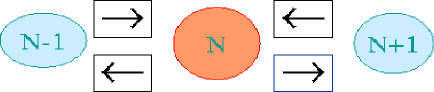
Figure 9: A schematic view of the master equation for the probability $P_{N}(\tau)$ due to $ab\leftrightarrow c\bar{c}$ and the inverse process.

The rate equation is determined by the magnitude of the transition probability per unit time due to the production $G/V$ and the absorption $L/V$ of $c\bar{c}$ pairs through $ab\leftrightarrow c\bar{c}$ process. The gain $(G=<\sigma_{ab\to c\bar{c}}v_{ab}>)$ and the loss $(L=<\sigma_{c\bar{c}\to ab}v_{c\bar{c}}>)$ terms represent the momentum average of particle production and absorption cross sections.

The transition probability per unit time from $N_{c}+1\to N_{c}$ is given by the product of the probability $L/V$ that the single reaction $c\bar{c}\to ab$ takes place multiplied by the number of possible reactions which is formally, $(N_{c}+1)(N_{\bar{c}}+1)$. In the case when the charge carried by particles $c$ and $\bar{c}$ is exactly and locally conserved, that is if $(N_{c}+N_{\bar{c}}=0$), this factor is just $(N_{c}+1)^{2}$. Similarly, the transition probability from $N_{c}\to N_{c}+1$ is described by $G\langle N_{a}\rangle\langle N_{b}\rangle/V$, where one assumes that particles $a$ and $b$ are not correlated and their multiplicity is governed by the thermal averages. One also assumes that the multiplicity of $a$ and $b$ is not affected by the $ab\to c\bar{c}$ process. The master equation for the time evolution of the probability $P_{N_{c}}(\tau)$ can be written[99] in the following form:

$$\frac{dP_{N_{c}}}{d\tau} = {G\over V}\langle N_{a}\rangle\langle N_{b}\rangle P_{N_{c}-1}+\frac{L}{V}(N_{c}+1)^{2}P_{N_{c}+1}$$ (15)

$$- {G\over V}\langle N_{a}\rangle\langle N_{b}\rangle P_{N_{c}}~{}~{}~{}-\frac{L}{V}N_{c}^{2}P_{N_{c}}.$$

The first two terms in Eq. (15) describe the increase of $P_{N_{c}}(\tau)$ due to the transition from $N_{c}-1$ and $N_{c}+1$ to the $N_{c}$ state. The last two terms, on the other hand, represent the decrease of the probability function due to the transition from $N_{c}$ to the $N_{c}+1$ and $N_{c}-1$ states, respectively.

For a thermal particle momentum distribution and under the Boltzmann approximation the thermal averaged cross sections are obrained[32, 31] from

$$<\sigma_{ab\to c\bar{c}}v_{ab}>={\beta\over 8}{{\int_{t_{0}}^{\infty}dt\sigma_{ab\to c\bar{c}}(t)[t^{2}-(m_{ab}^{+})^{2}][t^{2}-(m_{ab}^{-})^{2}]K_{1}(\beta t)}\over{m_{a}^{2}m_{b}^{2}K_{2}(\beta m_{a})K_{2}(\beta m_{b})}},$$ (16)

where $K_{1}$, $K_{2}$ are modified Bessel functions of the second kind, $m_{ab}^{+}=m_{a}+m_{b}$ and $m_{ab}^{-}=m_{a}-m_{b}$, $t=\sqrt{s}$ is the center-of-mass energy, $\beta$ the inverse temperature, $v_{ab}=((k_{a}k_{b})^{2}-m_{a}^{2}m_{b}^{2})/E_{a}E_{b}$ is the relative velocity of incoming particles and the integration limit is taken to be $t_{0}=max[(m_{a}+m_{b}),(m_{c}+m_{\bar{c}})]$.

The rate equation for probabilities (15) provides the basis to calculate the time evolution of the momentum averages of particle multiplicities and their arbitrary moments. Indeed, multiplying the above equation by $N_{c}$ and summing over $N_{c}$, one obtains the general kinetic equation for the time evolution of the average number $\langle N_{c}\rangle=\sum_{N_{c}=0}^{\infty}N_{c}P_{N_{c}}(\tau)$ of particles $c$ in a system. This equation reads:

$$\frac{d\langle N_{c}\rangle}{d\tau}={G\over V}\langle N_{a}\rangle\langle N_{b}\rangle-\frac{L}{V}\langle N_{c}^{2}\rangle.$$ (17)

The above equation cannot be solved analytically as it connects particle multiplicity $\langle N_{c}\rangle$ with its second moment $\langle N_{c}^{2}\rangle$. However, solutions can be obtained in two limiting situations: i) for an abundant production of $c$ particles, that is when $\langle N_{c}\rangle\gg 1$ or ii) in the opposite limit of rare particle production corresponding to $\langle N_{c}\rangle\ll 1$. Indeed, since

$${\langle N_{c}^{2}\rangle}=\langle N_{c}\rangle^{2}+\langle\delta N_{c}^{2}\rangle,$$ (18)

where $\langle\delta N_{c}^{2}\rangle$ represents the fluctuations of the number of particles $c$, one can make the following approximations:

i) for $\langle N_{c}\rangle\gg 1$ one has a $\langle N_{c}^{2}\rangle\approx\langle N_{c}\rangle^{2},$ and Eq. (17) obviously reduces to the well known[31] form:

$$\frac{d\langle N_{c}\rangle}{d\tau}\approx{G\over V}\langle N_{a}\rangle\langle N_{b}\rangle-\frac{L}{V}\langle N_{c}\rangle^{2}.$$ (19)

ii) however, for the rare production, particles $c$ and $\bar{c}$ are strongly correlated and thus, for $\langle N_{c}\rangle\ll 1$ one takes $\langle N_{c}^{2}\rangle\approx\langle N_{c}\rangle$, consequently Eq. (17) takes the form:

$$\frac{d\langle N_{c}\rangle}{d\tau}\approx{G\over V}\langle N_{a}\rangle\langle N_{b}\rangle-\frac{L}{V}\langle N_{c}\rangle,$$ (20)

where the absorption term depends only linearly, instead of quadratically, on the particle multiplicity.

From the above it is thus clear that, depending on the thermal conditions in the system (that is its volume and temperature), we are getting different results for the equilibrium solution and the time evolution of the number of produced particles $c$. This is very transparent when solving the rate equations (19) and (20).

In the limit when $\langle N_{c}\rangle\gg 1$, the standard Eq. (19) is valid and has the well known solution[99, 31]:

$$\langle N_{c}(\tau)\rangle=\langle N_{c}\rangle_{\rm eq}\tanh\left(\tau/\tau_{0}\right),$$ (21)

where the equilibrium value $\langle N_{c}\rangle_{\rm eq}$ of the number of particles $c$ and the relaxation time constant $\tau_{0}$ are given by:

$$\langle N_{c}\rangle_{\rm eq}=\sqrt{\epsilon}~{}~{},~{}~{}\tau_{0}=\frac{V}{L\sqrt{\epsilon}},$$ (22)

respectively, with $\epsilon=G\langle N_{a}\rangle\langle N_{b}\rangle/L$.

In the particular case when the particle momentum distribution is thermal, the ratio of the gain ($G$) to the loss ($L$) terms can be obtained [99] from Eq. (16) as

$$\frac{G}{L}=\frac{d_{c}m_{c}^{2}K_{2}(m_{c}/T)d_{\bar{c}}m_{\bar{c}}^{2}K_{2}(m_{\bar{c}}/T)}{d_{a}m_{a}^{2}K_{2}(m_{a}/T)d_{b}m_{b}^{2}K_{2}(m_{b}/T)},$$ (23)

where we have employed the detailed balance relation between the cross sections for production $\sigma_{ab}$ and for absorbtion $\sigma_{c\bar{c}}$ for $ab\leftrightarrow c\bar{c}$ processes

$$\sigma_{ab\to c\bar{c}}(t)={{d_{a}d_{b}}\over{d_{c}d_{\bar{c}}}}{{[t^{2}-(m_{c\bar{c}}^{+})^{2}][t^{2}-(m_{c\bar{c}}^{-})^{2}]}\over{[t^{2}-(m_{ab}^{+})^{2}][t^{2}-(m_{ab}^{-})^{2}]}}\sigma_{c\bar{c}\to ab}(t)$$ (24)

with $d_{i}$ being the spin-isospin degeneracy factor and $m^{\pm}_{ij}$ as in Eq. (16).

In Boltzmann approximation, the equilibrium average number of particles $c$ in Eq. (22) reads:

$$\langle N_{c}\rangle_{\rm eq}={{d_{c}}\over{2\pi^{2}}}VTm_{c}^{2}K_{2}(m_{c}/T).$$ (25)

This is a well known result for the average number of particles in the Grand Canonical (GC) ensemble with respect to the U(1) internal symmetry of the Hamiltonian. The chemical potential, which is usually present in the GC ensemble, vanishes in this case, because of the requirement of charge neutrality of the system. Thus, the solution of Eq. (19) results in the expected value for the equilibrium limit in the GC formalism where a charge is conserved on the average.

In the opposite limit, where $\langle N_{c}\rangle\ll 1$, the time evolution of a particle abundance is described by Eq. (20), that has the following solution:

$$\langle N_{c}(\tau)\rangle^{\rm C}=\langle N_{c}\rangle_{\rm eq}^{\rm C}\left(1-e^{-\tau/\tau_{0}^{\rm C}}\right),$$ (26)

with the equilibrium value and relaxation time given by

$$\langle N_{c}\rangle_{\rm eq}^{\rm C}=\epsilon,~{}\tau_{0}^{\rm C}=\frac{V}{L}.$$ (27)

The above result, as will be shown in the next section, is the asymptotic limit of the particle multiplicity obtained in the canonical (C) formulation of the conservation laws[99, 100]. Here the charge related with the U(1) symmetry is exactly and locally conserved, contrary to the GC formulation where this conservation is only valid on the average.

Comparing Eq. (22) with Eq. (27), we first find that, for $\langle N_{c}\rangle\ll 1$, the equilibrium value is by far smaller than what is obtained in the grand canonical limit, i.e.

$$\langle N_{c}\rangle_{\rm eq}^{\rm C}={\langle N_{c}\rangle_{\rm eq}}^{2}\ll{\langle N_{c}\rangle_{\rm eq}}.$$ (28)

Secondly, we can conclude that the relaxation time for a canonical system is shorter than the grand canonical value, i.e.

$$\tau_{0}^{\rm C}=\tau_{0}\langle N_{c}\rangle_{\rm eq}\ll\tau_{0},$$ (29)

since in the limit $\bf(ii)$ the equilibrium value $\langle N_{c}\rangle_{\rm eq}\ll 1$.

We note that the $(\bf i)$ and the $(\bf ii)$ limits are essentially determined by the size of $\langle\delta N_{c}^{2}\rangle$, the fluctuations of the number of particles $c$. The grand canonical results correspond to small fluctuations, i.e. $\langle\delta N_{c}^{2}\rangle/\langle N_{c}\rangle^{2}\leq 1$, while large fluctuations $\langle\delta N_{c}^{2}\rangle/\langle N_{c}\rangle^{2}$ $\geq 1$ require a canonical description.

The volume dependence of particle density obviously differs in the C and in the GC limit. The particle density in the GC limit is $V$-independent whereas in the canonical approach it can even scale linearly with $V$.

The difference between the C and asymptotic GC result already seen on the level of the rate equations (17,19), is even more transparent when comparing master equations for probabilities. In the following we formulate this equation for the GC description of quantum number conservation.

In case of abundantly produced particles $c$ and $\bar{c}$ through the $ab\to c\bar{c}$ process we do not need to worry about strong particle correlations due to charge conservation. This also means that, instead of imposing charge neutrality conditions through $N_{c}-N_{\bar{c}}=0$, one assumes conservation on the average, that is $\langle N_{c}\rangle-\langle N_{\bar{c}}\rangle=0$. In this case the master equation (15) can be simplified.

In the derivation of Eq. (15) the absorption terms proportional to $L$ were obtained by constraining the charge conservation to be local and exact. For the conservation on the average, the transition probability from $N_{c}$ to the $(N_{c}-1)$ state is no longer proportional to $(L/V)N_{c}^{2}$ but rather to $(L/V)N_{c}\langle N_{\bar{c}}\rangle$, since the exact conservation condition $N_{c}=N_{\bar{c}}$ is no longer valid and the number of $\bar{c}$ particles can only be determined by its average value. In the GC limit, the master equation for the time evolution of the probability $P_{N_{c}}(\tau)$ takes the following form:

$$\frac{dP_{N_{c}}}{d\tau} = {G\over V}\langle N_{a}\rangle\langle N_{b}\rangle P_{N_{c}-1}+\frac{L}{V}(N_{c}+1)\langle N_{\bar{c}}\rangle P_{N_{c}+1}$$ (30)

$$- {G\over V}\langle N_{a}\rangle\langle N_{b}\rangle P_{N_{c}}~{}~{}~{}-\frac{L}{V}N_{c}\langle N_{\bar{c}}\rangle P_{N_{c}}.$$

Multiplying the above equation by $N_{c}$, summing over $N_{c}$ and using the condition that $\langle N_{c}\rangle=\langle N_{\bar{c}}\rangle$, one recovers Eq. (19), the rate equation for $\langle N_{c}\rangle$ in the GC ensemble. The above equation is thus indeed the general master equation for the probability function in the GC limit. Comparing this equation with the more general Eq. (15), one can see that the main difference is contained in the absorption terms that are linear in particle number instead of being quadratic .

Eq. (30) can be solved exactly. Indeed, introducing the generating function $g(x,\tau)$ for $P_{N_{c}}$,

$$g(x,{\tau})=\sum_{N_{c}=0}^{\infty}x^{N_{c}}P_{N_{c}}(\tau),$$ (31)

the iterative equation (30) for the probability can be converted into a differential equation for the generating function:

$$\frac{\partial g(x,\tau)}{\partial\tau}={{L}\over V}\sqrt{\epsilon}(1-x)[g^{\prime}-{\sqrt{\epsilon}}g],$$ (32)

with the general solution[99]:

$$g(x,\tau)=g_{0}(1-xe^{-\tilde{\tau}})\exp[{\sqrt{\epsilon}(1-x)(e^{-\tilde{\tau}}-1)}],$$ (33)

where $g^{\prime}=\partial g/\partial x$, $\tilde{\tau}=(L\sqrt{\epsilon}/V)\tau$ and $\sqrt{\epsilon}=\langle N_{c}\rangle_{eq}$ given by Eq. (9).

One can readily find out an equilibrium solution to the above equation. Taking the limit $\tau=\infty$ in the Eq. (33) leads to

$$g_{\rm eq}(x)=\exp[{-\sqrt{\epsilon}(1-x)}],$$ (34)

with the corresponding equilibrium multiplicity distribution:

$$P_{N_{c},{\rm eq}}=\frac{(\sqrt{\epsilon})^{N_{c}}}{{N_{c}}!}e^{-\sqrt{\epsilon}}.$$ (35)

This is the expected Poisson distribution with average multiplicity $\sqrt{\epsilon}$.

3.1.2 The equilibrium solution of the general rate equation

The master equation (30), that describes the evolution of the probability function in the GC limit, could be solved analytically. The general equation (15), however, because of the quadratic dependence of the absorption terms, requires a numerical solution. Nevertheless, the equilibrium result for the particle multiplicity can be given.

Converting Eq. (15) for $P_{N_{c}}$ into a partial differential equation for the generating function

$$g(x,\tau)=\sum_{N_{c}=0}^{\infty}x^{N_{c}}P_{N_{c}}(\tau).$$ (36)

one finds[99]

$$\frac{\partial g(x,\tau)}{\partial\tau}=\frac{L}{V}(1-x)\left(xg^{\prime\prime}+g^{\prime}-\epsilon g\right).$$ (37)

The equilibrium solution $g_{\rm eq}(x)$ thus obeys the following equation:

$$xg_{\rm eq}^{\prime\prime}+g_{\rm eq}^{\prime}-\epsilon g_{\rm eq}=0.$$ (38)

By a substitution of variables ($x=y^{2}\epsilon/4$), this equation is reduced to the Bessel equation, with the following solution:

$$g_{\rm eq}(x)=\frac{1}{I_{0}(2\sqrt{\epsilon})}I_{0}(2\sqrt{\epsilon x}),$$ (39)

where the normalization is fixed by $g(1)=\sum P_{N_{c}}=1$.

The equilibrium value for the probability function $P_{N_{c}}$ is now written from Eqs. (36–39) as:

$$P_{N_{c},\rm eq}=\frac{\epsilon^{N_{c}}}{I_{0}(2\sqrt{\epsilon})(N_{c}!)^{2}}.$$ (40)

We note that the equilibrium distribution of the particle multiplicity is not Poissonian. This fact was indicated first in equilibrium studies in Ref. (r39). In our case this is a direct consequence of the quadratic dependence on the multiplicity in the loss terms of the master equation (15). The Poisson distribution is obtained from Eq. (40) if $\sqrt{\epsilon}\gg 1$, that is for large particle multiplicity where the C ensemble coincides with the GC asymptotic approximation. In Fig. (10) we compare the Poisson distribution from Eq. (35) with the distribution from Eq. (40) for two values of $\sqrt{\epsilon}$.

Figure 10: The probability function from Eqs. (35,40) for two values of $\epsilon=4$ and 16. The full lines represent Poisson distribution.

The result for the equilibrium average number of particles $c$ can be obtained as:

$$\langle N_{c}\rangle_{\rm eq}=g^{\prime}(1)=\sqrt{\epsilon}\frac{I_{1}(2\sqrt{\epsilon})}{I_{0}(2\sqrt{\epsilon})}.$$ (41)

The above expression will be shown in the next section to coincide with the one expected for the particle multiplicity in the canonical ensemble with respect to U(1) charge conservation[105, 106]. The rate equation formulated in Eq. (15) is valid for arbitrary values of $\langle N_{c}\rangle$ and obviously reproduces (see Eqs. (101 - 104)) the standard grand canonical result for a large $\langle N_{c}\rangle$. Thus, within the approach developed above one can study the chemical equilibration of charged particles following Eq. (15), independent of thermal conditions inside the system.

3.1.3 The master equation in the presence of the net charge.

So far, in constructing the evolution equation for probabilities, we have assumed that there is no net charge in the system under consideration. For the application of the statistical approach to particle production in heavy ion and hadron–hadron collisions, the above assumption has to be extended to the more general case of non–vanishing initial values of conserved charges. In the following we construct the evolution equation for $P_{N_{c}}^{S}(t)$ in a thermal medium assuming that its net charge $S$ is non–vanishing.

The presence of a non–zero net charge requires modification of the absorption terms in Eq. (15). The transition probability per unit time from the $N_{c}$ to the $N_{c}-1$ state was proportional to $(L/V)N_{c}N_{\bar{c}}$. Admitting an overall net charge $S\neq 0$ the exact charge conservation implies that $N_{c}-N_{\bar{c}}=S$. The transition probability from $N_{c}$ to $N_{c}-1$ due to pair annihilation is thus $(L/V)N_{c}(N_{c}-S)$. Following the same procedure as in Eq. (15) one can formulate the following master equation for the probability $P_{N_{c}}^{S}(t)$ to find $N_{c}$ particles $c$ in a thermal medium with a net charge $S$:

$$\frac{dP_{N_{c}}^{S}}{d\tau} = {G\over V}\langle N_{a}\rangle\langle N_{b}\rangle P_{N_{c}-1}^{S}+\frac{L}{V}(N_{c}+1)(N_{c}+1-S)P_{N_{c}+1}^{S}$$ (42)

$$- {G\over V}\langle N_{a}\rangle\langle N_{b}\rangle P_{N_{c}}^{S}~{}~{}~{}-\frac{L}{V}N_{c}(N_{c}-S)P_{N_{c}}^{S},$$

which obviously reduces to Eq. (15) for $S=0$.

To get the equilibrium solution for the probability and multiplicity, we again convert the above equation to the differential form for the generating function $g^{S}(x,\tau)=\sum_{N_{c}=0}^{\infty}x^{N_{c}}P_{N_{c}}^{S}(\tau)$:

$$\frac{\partial g^{S}(x,\tau)}{\partial\tau}=\frac{L}{V}(1-x)\left(xg_{S}^{\prime\prime}+g_{S}^{\prime}(1-S)-\epsilon g_{S}\right).$$ (43)

In equilibrium, ${\partial g^{S}(x,\tau)}{\partial\tau}=0$ and the solution for $g^{S}_{\rm eq}$ can be found as follows:

$$g^{S}_{\rm eq}(x)=\frac{x^{S/2}}{I_{S}(2\sqrt{\epsilon})}I_{S}(2\sqrt{\epsilon x}),$$ (44)

where the normalization is fixed by $g(1)=\sum P_{n}=1$.

The master equation for the probability to find $N_{\bar{c}}$ antiparticles $\bar{c}$, its corresponding differential form and the equilibrium solution for the generating function can be obtained by replacing $S$ with $-S$ in Eqs. (42–44)

The result for the equilibrium average number of particles $\langle N_{c}\rangle_{\rm eq}$ and antiparticles $\langle N_{\bar{c}}\rangle_{\rm eq}$ is obtained from the generating function using the relation: $\langle N_{c}\rangle_{\rm eq}=g^{\prime}(1)$. The final expressions read:

$$\langle N_{c}\rangle_{\rm eq}=\sqrt{\epsilon}\frac{I_{S-1}(2\sqrt{\epsilon})}{I_{S}(2\sqrt{\epsilon})}~{}~{},~{}~{}\langle N_{\bar{c}}\rangle_{\rm eq}=\sqrt{\epsilon}\frac{I_{S+1}(2\sqrt{\epsilon})}{I_{S}(2\sqrt{\epsilon})}.$$ (45)

The charge conservation is explicitly seen by taking the difference of these equations that results in the net value of the charge $S$.

The thermal average values of the particle number given through Eq. (45) will be later derived from the equilibrium partition function by using the projection method[106, 107].

3.1.4 The kinetic equation for different particle species

The rate equations discussed until now were derived assuming that there is only one kind of particle $c$ and its antiparticle $\bar{c}$ that carry conserved charge. To study equilibration of particles in a strongly interacting environment one also needs to include processes that involve different species. In low energy heavy ion collisions e.g. the $K^{+}$ mesons are not only produced in pairs together with $K^{-}$ but also with the strange hyperon $\Lambda$ or $\Sigma^{0}$ due to the $\pi N\to\Lambda K^{+}$ process. The contribution of $K^{0}$ and $\bar{K^{0}}$ has to be also included as these particles are produced with similar strength as charged kaons. To account for this situation one generalizes the rate equations described in the last sections.

Consider $P_{N_{K},N_{\Lambda}}(\tau)$ as the probability to find $N_{K}$ and $N_{\Lambda}$ number of $K^{-}$ mesons and $\Lambda$ baryons. Including the production and absorption processes such as: $m\bar{m}\to K^{+}K^{-}$ and $mN\to K^{+}\Lambda$ this probability will obviously change in time. Here $m(N)$ denotes a meson (nucleon).

Following a similar procedure as was explained in Fig. (9) the master equation for the time evolution of the probability $P_{N_{K},N_{\Lambda}}(\tau)$ can be written as:[100, 101]

$$\frac{P_{N_{K},N_{\Lambda}}}{d\tau} = {G_{m}\over V}\langle N_{m}\rangle\langle N_{\bar{m}}\rangle P_{N_{K}-1,N_{\Lambda}}+\frac{L_{m}}{V}(N_{K}+1)(N_{K}+1+N_{\Lambda})$$

$$\times P_{N_{K}+1,N_{\Lambda}}$$

$$- {G_{m}\over V}\langle N_{m}\rangle\langle N_{\bar{m}}\rangle P_{N_{K},N_{\Lambda}}~{}~{}~{}-\frac{L_{m}}{V}N_{K}(N_{K}+N_{\Lambda})P_{N_{K},N_{\Lambda}}$$

$$+ {G_{N}\over V}\langle N_{m}\rangle\langle N_{N}\rangle P_{N_{K},N_{\Lambda}-1}+\frac{L_{N}}{V}(N_{\Lambda}+1)(N_{\Lambda}+1+N_{K})$$

$$\times P_{N_{K},N_{\Lambda}+1}$$

$$- {G_{N}\over V}\langle N_{m}\rangle\langle N_{N}\rangle P_{N_{K},N_{\Lambda}}~{}~{}~{}-\frac{L_{N}}{V}N_{\Lambda}(N_{\Lambda}+N_{K})P_{N_{K},N_{\Lambda}}.$$

with $G_{m}$ and $L_{m}$ being the production and absorption terms for the $m\bar{m}\rightleftharpoons K^{+}K^{-}$ reaction and $G_{N}$ and $L_{N}$ denote equivalent terms for the $mN\rightleftharpoons K^{+}\Lambda$ process.

The equilibrium solution for the probability function $P_{N_{K}N_{\Lambda}}$ can be found as follows[101]:

$$P_{N_{K},N_{\Lambda}}=\frac{\epsilon_{tot}^{N_{K}+N_{\Lambda}}}{I_{0}(2\sqrt{\epsilon_{tot}})((N_{K}+N_{\Lambda})!)^{2}}\frac{(N_{K}+N_{\Lambda})!\epsilon_{m}^{N_{K}}\epsilon_{N}^{N_{\Lambda}}}{\epsilon_{tot}^{N_{K}+N_{\Lambda}}N_{K}!N_{\Lambda}!}$$ (47)

with $\epsilon_{tot}=\epsilon_{m}+\epsilon_{N}$ and $\epsilon_{m(N)}=G_{m(N)}\langle N_{m_{1}(m)}\rangle\langle N_{m_{2}(N)}\rangle/L_{m(N)}$.

The equilibrium probability distribution is thus, according to Eq. (47), the product of the distribution of the number of pairs $(N_{K}+N_{\Lambda})$ and a binomial distribution that determines the relative weight of the individual particles, in our case the $K^{-}$ and $\Lambda$.

The probability $P_{i,j}$ is obviously normalized such that $\sum_{i,j}P_{i,j}=1$. The equilibrium value for the multiplicity $\langle N_{i}\rangle$ with $i=K^{-}$ or $i=\Lambda$ can be obtained as:

$$\langle N_{K^{-}}\rangle_{\rm eq}={{\epsilon_{m}}\over\sqrt{\epsilon}_{tot}}\frac{I_{1}(2\sqrt{\epsilon_{tot}})}{I_{0}(2\sqrt{\epsilon_{tot}})}~{}~{},~{}~{}\langle N_{\Lambda}\rangle_{\rm eq}={{\epsilon_{N}}\over\sqrt{\epsilon}_{tot}}\frac{I_{1}(2\sqrt{\epsilon_{tot}})}{I_{0}(2\sqrt{\epsilon_{tot}})}$$ (48)

with $\epsilon_{m},\epsilon_{N}$ and $\epsilon_{tot}$ defined as above.

The average value of $K^{+}$ can be obtained applying strangeness conservation leading to:

$$\langle N_{K^{+}}\rangle_{eq}=\langle N_{K^{-}}\rangle_{eq}+\langle N_{\Lambda}\rangle_{eq}.$$ (49)

The results presented here can be extended[101] to an even more general case where there is an arbitrary number of different particle species carrying the quantum numbers related with U(1) symmetry of the Hamiltonian.

3.2 The canonical description of an internal symmetry - projection method

Using the above kinetic analysis of charged particle production probabilities we have demonstrated that equilibrium distributions does not necessarily coincide with the GC value. It is thus natural to ask what is the corresponding partition function that can reproduce the kinetic results obtained in Eqs. (41,45,48). The main step in deriving these equations was an assumption of an exact conservation of quantum numbers in the kinetic master equations (15,42,3.1.4). Thus, one should account for this important constraint in constructing the partition function.

The exact treatment of quantum numbers in statistical mechanics has been well established[105, 106] for some time now. It is in general obtained[107, 108] by projecting the partition function onto the desired values of the conserved charge by using group theoretical methods. In this section we develop these methods and show how one gets the partition function that accounts for exact conservation of quantum numbers. The derivation will be not only restricted to the charge conservation related with an Abelian U(1) internal symmetries and their direct products, but it will include also symmetries that are imposed by any semi-simple compact Lie group.

The usual way of treating the problem of quantum number conservation in statistical physics is by introducing the grand canonical partition function, as in Eq. (3). For only one conserved charge, e.g. strangeness $S$,

$$Z(\mu_{S},T)={\rm Tr}[e^{-\beta(\hat{H}-\mu_{S}\hat{S})}]$$ (50)

The chemical potential $\mu_{S}$ is then fixed by the condition that the average value of strangeness of a thermodynamical system is conserved and has the required value $\langle S\rangle$ such that:

$$\langle S\rangle=T{{\partial\ln Z(\mu_{S},T)}\over{\partial\mu_{S}}}$$ (51)

This method, as shown in the previous sections, is only adequate if the number of particles carrying strangeness is very large and their fluctuations can be neglected.

In order to derive a partition function that is free from the above requirements let us first reorganize Eq. (50). Denoting the states under the trace as $\vline s\rangle$ such that $\hat{H}\vline s\rangle=E_{s}\vline s\rangle$ and $\hat{S}\vline s\rangle=s\vline s\rangle$ one writes

$$Z(\mu_{S},T)=\sum_{s=-\infty}^{s=+\infty}e^{-\beta E_{s}}e^{s\beta\mu_{S}}=\sum_{s=-\infty}^{s=+\infty}Z_{S}\lambda_{S}^{s}$$ (52)

where we have introduced the fugacity $\lambda_{S}=e^{\beta\mu_{S}}$ and where

$$Z_{S}={\rm Tr_{S}}[e^{-\beta\hat{H}}]$$ (53)

is just the partition function that is restricted to a specific total value $S$ of the conserved charge. This is the canonical partition function with respect to strangeness conservation. Thus, $Z_{S}$ is a coefficient in the Laurent series in the fugacity. Our goal is to calculate $Z_{S}$. This is an easy task: starting from Eq. (52) we apply the Cauchy formula and take an inverse transformation to obtain

$$Z_{S}(T,V)={{1}\over{2\pi i}}\oint{{d\lambda_{S}}\over{\lambda_{S}^{s+1}}}Z(\lambda_{S},T,V)$$ (54)

Choosing the integration path as the unit circle and parameterizing it as $\lambda_{S}=\exp{(i\phi)}$ we can convert the contour integral into the angular one as

$$Z_{S}(T,V)=\int_{-\pi}^{+\pi}{{d\phi}\over{2\pi}}\tilde{Z}(\phi,T,V)$$ (55)

where the generating function $\tilde{Z}(\phi,T,V)=Z(\lambda_{S}=e^{i\phi},T,V)$ is obtained from the grand canonical partition function by a Wick rotation of the chemical potential $\mu_{S}\to i\phi$. This generating function is the same for all canonical partition functions with an arbitrary but fixed value of the conserved charge. Eq. (55) is the projection formula onto the canonical partition function that accounts for the exact conservation of an Abelian charge. This is a projection procedure as $Z_{S}$ is obtained from

$$Z_{S}(T,V)={\rm Tr_{S}}[e^{-\beta\hat{H}}]={\rm Tr}[e^{-\beta\hat{H}}P_{S}]$$ (56)

where $P_{S}=P_{S}^{2}$ is the projection operator on the states with the exact value of $S$. For an Abelian symmetry, $P_{S}$ is the $\delta$–function $P_{S}=\delta_{\hat{S},S}$. Introducing the Fourier decomposition of delta into Eq. (56) one can reproduce the projected result (55).

The conservation of additive quantum numbers like baryon number, strangeness, electric charge or charm is related to the invariance of the Hamiltonian under the U(1) Lie group. In many applications it is important to generalize the projection method to symmetries that are related with a non-Abelian Lie group $G$. An example is the special unitary group SU(N) that plays an essential role in the theory of strong interactions. Generalization of the projection method would require to specify the projection operator or generating function. Consequently, the partition function obtained with the specific eigenvalues of the Casimir operators that fixes the multiplet of the irreducible representation of the symmetry group $G$ could be determined.

To find the generating function for the canonical partition function with respect to the symmetry group $G$, let us introduce the quantity $\tilde{Z}(g)$ via

$$\tilde{Z}(g)={\rm Tr}[U(g)e^{-\beta\hat{H}}].$$ (57)

This expression is a function on the group $G$ with U(g) being the unitary representation of the group with $g\subset G$. The quantity U(g) can be decomposed into irreducible representations $U_{\alpha}(g)$

$$U(g)=\sum_{\alpha}^{\bigoplus}U_{\alpha}(g)$$ (58)

where $\alpha$ is labelling these representations. From Eq. (57) and (58) one has

$$\tilde{Z}(g) = \sum_{\alpha}{\rm Tr_{\alpha}}[U_{\alpha}(g)e^{-\beta\hat{H}}]$$ (59)

$$= \sum_{\alpha}\sum_{\nu_{\alpha},\xi_{\alpha}}\langle\nu_{\alpha},\xi_{\alpha}\mid U_{\alpha}(g)e^{-\beta\hat{H}}\mid\nu_{\alpha},\xi_{\alpha}\rangle$$

where $\nu_{\alpha}$ labels the states within the representation $\alpha$ and $\xi_{\alpha}$ are degeneracy parameters.

Introducing the unit operator $1=\mid\rangle\langle\mid$ into the above equation the expression factorizes

$$\tilde{Z}(g) = \sum_{\alpha}\sum_{\nu_{\alpha},\xi_{\alpha}}\langle\nu_{\alpha},\xi_{\alpha}\mid U_{\alpha}(g)\mid\nu_{\alpha},\xi_{\alpha}\rangle\langle\nu_{\alpha},\xi_{\alpha}\mid e^{-\beta\hat{H}}\mid\nu_{\alpha},\xi_{\alpha}\rangle$$ (60)

$$= \sum_{\alpha}\sum_{\nu_{\alpha},\xi_{\alpha}}\langle\nu_{\alpha}\mid U_{\alpha}(g)\mid\nu_{\alpha}\rangle\langle\xi_{\alpha}\mid e^{-\beta\hat{H}}\mid\xi_{\alpha}\rangle,$$

where we have used that, due to the exact symmetry, the only non–vanishing matrix elements of $e^{-\beta\hat{H}}$ are those diagonal in $\nu_{\alpha}$. The matrix elements of $U_{\alpha}(g)$ are only non-zero if they are diagonal in $\xi_{\alpha}$. Finally, the matrix elements of the Hamiltonian are independent of the states within representation (since due to symmetry they are dynamically equivalent) and those of $U(g)$ of degeneracy factors (since $U(g)$ does not distinguish dynamically different states that transform under the same representation).

The last two sums in Eq. (60) can be further simplified as

$$\sum_{\nu_{\alpha}}\langle\nu_{\alpha}\mid U_{\alpha}(g)\mid\nu_{\alpha}\rangle={\rm Tr_{\alpha}}[U_{\alpha}(g)]=\chi_{\alpha}(g).$$ (61)

The quantity $\chi_{\alpha}$ is by definition the character of the irreducible $U_{\alpha}(g)$ representation and

$$\sum_{\xi_{\alpha}}\langle\xi_{\alpha}\mid e^{-\beta\hat{H}}\mid\xi_{\alpha}\rangle={{1}\over{d(\alpha)}}{\rm Tr_{\alpha}}e^{-\beta\hat{H}}={{1}\over{d(\alpha)}}Z_{\alpha}(T,V),$$ (62)

where $Z_{\alpha}$ is the canonical partition function with respect to the $G$ symmetry of the Hamiltonian and $d(\alpha)$ is the dimension of the representation $\alpha$. Calculating $Z_{\alpha}$ one considers under the trace only those states that transform with respect to a given irreducible representation of the symmetry group.

We have thus connected, through Eq. (60) and (61–62), the canonical partition function with the generating functional on the group

$$\tilde{Z}(g)=\sum_{\alpha}{{\chi_{\alpha}(g)}\over{d(\alpha)}}Z_{\alpha}(T,V)$$ (63)

The canonical partition function is the coefficient in the cluster decomposition of the generating function with respect to the characters of the representations.

The character functions satisfy the orthogonality relation

$${1\over{d(\alpha})}\int d\mu(g)\chi_{\alpha}^{*}(g)\chi_{\gamma}(g)=\delta_{\alpha,\gamma}$$ (64)

where $d\mu(g)$ is an invariant Haar measure on the group.

The orthogonality relation for characters allows to find the coefficients, the canonical partition function, in this cluster decomposition. From Eq. (63) and (64) one gets

$$Z_{\alpha}(T,V)=d(\alpha)\int d\mu(g){\chi_{\alpha}^{*}(g)}\tilde{Z}(g)$$ (65)

This result is a generalization of Eq. (55) to an arbitrary symmetry group that is a compact Lie group. The formula holds for any dynamical system described by the Hamiltonian $H$.

To find the canonical partition function we have to determine first the generating function $\tilde{Z}(g)$ defined on the symmetry group $G$. If the symmetry group is of rank $r$, then the character of any irreducible representation are the functions of $r$ variables $\{\gamma_{1},_{....},\gamma_{r}\}$. Denoting as $J_{k}$ the commuting generators of $G$ with $k=1,...,r$ the character function

$$\chi_{\alpha}(\gamma_{1},..,\gamma_{r})=\sum_{\nu_{\alpha}}\langle\nu_{\alpha}\mid e^{i\sum_{i=1}^{i=r}\gamma_{i}J_{i}}\mid\nu_{\alpha}\rangle$$ (66)

is obtained. Here, $\nu_{\alpha}$ labels the state within the representation $\alpha$. With the above form of the characters we can write Eq. (63) as

$$\tilde{Z}(\gamma_{1},..,\gamma_{r})={\rm Tr}[e^{-\beta\hat{H}+i\sum_{i=1}^{i=r}\gamma_{i}J_{i}}]$$ (67)

Through the Wick rotation $\gamma_{i}=-i\beta\mu_{i}$ the generating function $\tilde{Z}$ is just the GC partition function with respect to the conservation laws given by all commuting generators of the symmetry group $G$.

The equations (65) and (67) are the basis that permits to obtain the canonical partition function for systems restricted to any symmetry. The simplicity of the projection formula (65) is that the operators that appear in the generating function are additive they are generators of the maximal Abelian subgroup of $G$. Thus, the problem of extracting the canonical partition function with respect to an arbitrary semi-simple compact Lie group $G$ is reduced to the projection onto a maximal Abelian subgroup of $G$.

The calculation of the generating function from the Eq. (67) can be done applying standard perturbative diagrammatic methods or a mean field approach. However, if interactions can be omitted or effectively described by a modification of the particle dispersion relations by implementing an effective mass, then the trace in Eq. (67) can be worked out[107] exactly, leading to

$$\tilde{Z}(\vec{\gamma})=\exp[{\sum_{\alpha}{{\chi_{\alpha}(\vec{\gamma})}\over{d(\alpha)}}Z^{1}_{\alpha}}]$$ (68)

where $\vec{\gamma}=(\gamma_{1},_{.}.,\gamma_{r})$ and $Z^{1}_{\alpha}=\int(gVdp/2\pi^{2})p^{2}\exp{(-\sqrt{p^{2}+m_{\alpha}^{2}}/T)}$ is just the thermal particle phase–space in Boltzmann approximation belonging to a given irreducible multiplet of a symmetry group $G$. The sum is taken over all particle representations that are constituents of the thermodynamical system.

3.2.1 Canonical models with a non-Abelian symmetry

To illustrate how the projection method described above works, we discuss a statistical model that accounts for the canonical conservation of non-Abelian charges related with the $SU_{c}$(N)$\times U_{B}(1)$ symmetry with $N=3$ and $B$ being the baryon number and $c$ denoting the global gauge colour symmetry.

Let us consider a thermal fireball that is composed of quarks and gluons at temperature T and volume V . We describe the canonical partition function that is projected on the global color singlet and exact value of the baryon number. The interactions between quarks and gluons are implemented effectively, resulting in dynamical particle masses that are temperature dependent, e.g. through $m_{q,(g)}\sim gT$. Since the interactions are only trivially modifying the dispersion relations one can still use the free particle momentum phase-space. Thus, under this assumption, Eq. (68) provides the correct description of the generating function. The sum in the exponents in (68) gets contributions from quarks, antiquarks and gluons that transform under the fundamental (0,1), their conjugate (1,0) and adjoint (1,1) representation of the $SU_{c}(N)\times U_{B}(1)$ symmetry group. Thus,

$$\ln\tilde{Z}(T,V,\vec{\gamma},\gamma_{B})={{\chi_{Q}}\over{d_{Q}}}Z_{Q}^{1}+{{\bar{\chi}_{Q}}\over{d_{Q}}}Z_{\bar{Q}}^{1}+{{\chi_{G}}\over{d_{G}}}Z_{G}^{1}$$ (69)

where $\vec{\gamma}=(\gamma_{1},..,\gamma_{N-1})$ are the parameters of the $SU_{c}(N)$ and $\gamma_{B}$ of the $U_{B}(1)$ symmetry group.

Through an explicit calculation of one-particle partition functions for massive quarks and gluons the corresponding generating function is obtained as

$$\ln\tilde{Z}_{Q}(T,V,\vec{\gamma},\gamma_{B}) = \frac{g_{Q}}{d_{Q}}\frac{m_{Q}^{2}VT}{2\pi^{2}}\sum_{n=0}^{\infty}\frac{(-1)^{n+1}}{{n^{2}}}K_{2}(m_{Q}/T)$$ (70)

$$[ e^{i\gamma_{B}n/T}\chi_{Q}(n\vec{\gamma})+e^{-i\gamma_{B}n/T}\chi_{Q}^{*}(n\vec{\gamma})]$$

where the two terms in the bracket represent the contribution of quarks and antiquarks, respectively. The corresponding result for massive gluons reads

$$\ln\tilde{Z}_{G}(T,V,\vec{\gamma},\gamma_{B})=\frac{g_{G}}{d_{G}}\frac{m_{G}^{2}VT}{2\pi^{2}}\sum_{n=0}^{\infty}\frac{1}{{n^{2}}}K_{2}(m_{G}/T)[\chi_{G}(n\vec{\gamma})+\chi_{Q}^{*}(n\vec{\gamma})]~{}~{}~{}~{}$$ (71)

where $g_{G},g_{Q}$ and $d_{Q}=N,d_{G}=N^{2}-1$, are respectively, the quark and gluon degeneracy factors and dimensions of the representations.

Now we can apply this generating function in the projection formula (65) to get the canonical partition function. Of particular interest is the color singlet partition function that represents global colour neutrality (phenomenological confinement) of a quark-gluon plasma droplet. The conjugate character for the $SU_{c}(N)$ singlet representation is particulary simple, $\chi^{(0,0)}=1$. The baryon number be treated grand canonically requiring a substitution $\gamma_{B}=-i\mu_{B}/T$ in Eq. (70). To find $\tilde{Z}$ one still needs an explicit form of the fundamental and adjoint characters and the Haar measure on the $SU_{c}(N)$ group. Here we quote their structure for the $SU_{c}(3)$ group. The real $L_{R}$ and the imaginary $L_{I}$ parts of the character in the fundamental (quark) representation are

$$L_{R}=\cos\gamma_{1}+\cos\gamma_{2}+\cos(\gamma_{1}+\gamma_{2})$$

$$L_{I}=\sin\gamma_{1}+\sin\gamma_{2}-\sin(\gamma_{1}+\gamma_{2}).$$

For the adjoint (gluon) representation

$$\chi_{G}=2[\cos(\gamma_{1}-\gamma_{2})+\cos(2\gamma_{1}+\gamma_{2})+\cos(2\gamma_{2}+\gamma_{1})+1].$$ (72)

The invariant Haar measure on the $SU_{c}(3)$ internal symmetry group

$$d\mu(\gamma_{1},\gamma_{2})=\frac{8}{3\pi^{2}}\sin^{2}(\frac{\gamma_{1}-\gamma_{2}}{2})\sin^{2}(\frac{2\gamma_{1}+\gamma_{2}}{2})\sin^{2}(\frac{2\gamma_{2}+\gamma_{1}}{2}).~{}~{}$$ (73)

From Eqs. (70)-(73) and (65) we write the final result for the $SU_{c}(3)$ color singlet partition function that for non-vanishing baryon chemical potential $\mu_{B}$ reads

$$Z^{0}(\mu_{B},T,V)=\int d\mu(\gamma_{1},\gamma_{2}) \exp\{c_{1}\chi_{G}+$$ (74)

$$c_{2}[L_{R}\cosh(\beta\mu_{B})+iL_{I}\sinh(\beta)]\}$$

where the constants $c_{1}$ and $c_{2}$ can be extracted from Eqs. (70–71).

The above partition function shows a complex structure of the integrand. However, due to its symmetry it is straightforward to show that the partition function is real. The thermodynamical properties of this color singlet canonical partition function and other thermodynamical observables can be studied[110, 111, 112] by a numerical analysis.

In finite temperature gauge theory the zero component of the gauge field $A_{0}$ takes on the role of the Lagrange multiplier guaranteeing that all states satisfy Gauss law. In Euclidean space one can choose a gauge in such a way that $A_{0}^{\nu}(x,\tau)\lambda_{\nu}$ is a constant in space-time. In such a gauge the Wilson loop defined as

$$L(x)={1\over N}{\rm Tr}P\exp[ig\int_{0}^{\beta}A_{0}(x,\tau)d\tau]$$ (75)

represents the character of the fundamental representation of the $SU_{c}(N)$ group[110].

The effective potential of the $SU(N)$ spin model for the Wilson loop in the above gauge coincides[110, 113] essentially with the generating function given in Eq. (74). In addition, this generating function could be also related to the strong coupling effective free energy of the lattice gauge theory with a finite chemical potential[110]. Thus, the effective model formulated above connects the colored quasi-particle degrees of freedom with the Wilson loop.

3.2.2 The canonical partition function for Abelian charges

In this section we show how the projection method described above leads to a description of particle yields under the constraints imposed by the Abelian $U_{B}(1)$ symmetry. In this case the formalism is particularly transparent due to a simple structure of the symmetry group.

The U(1) group is of rank one, thus the characters of the representations, numbered by the eigenvalues of the conserved charge B, depend only on one parameter $\phi$. They are of the exponential type:

$$\chi^{B}_{U_{B}(1)}=e^{iB\phi}.$$ (76)

For the conservation of a few Abelian charges inside the system like strangeness (S), baryon number (B) or electric charge (Q) and charm (C) one needs to account for the products of the U(1) symmetries: $U_{S}(1)\times U_{B}(1)\times U_{Q}(1)\times U_{C}(1)$. In this case the characters are numbered by the values of all conserved charges and they are expressed as the products of the corresponding characters of U(1) groups. For simultaneous conservation of baryon number and strangeness the characters read:

$$\chi^{S,B}_{U_{S}(1)\times U_{B}(1)}=\chi^{S}_{U_{S}(1)}\cdot\chi^{B}_{U_{B}(1)}=e^{i(S\psi+B\phi}).$$ (77)

The invariant measure on the $U_{S}(1)\times U_{B}(1)$ group is just the product of the differentials $d\mu(\phi_{S},\phi_{B})=(d\phi_{S}/2\pi)\cdot(d\phi_{B}/2\pi)$.

In nucleus-nucleus collisions the absolute values of the baryon number, electric charge and strangeness are fixed by the initial conditions. Modelling the particle production using statistical thermodynamics, in general, requires a canonical formulation of all these quantum numbers. We restrict our discussion only to the case when at most two conserved charges can be simultaneously canonical (e.g. the strangeness and baryon number) and all others are treated using the GC formulation. The corresponding canonical partition functions can be obtained from Eqs. (65,68) as:

$$Z_{S}={1\over{2\pi}}\int_{0}^{2\pi}d\phi e^{-iS\phi}{\tilde{Z}}(T,V,\phi)$$ (78)

and

$$Z_{B,S}={1\over{4\pi^{2}}}\int_{0}^{2\pi}d\phi e^{-iQ\phi}\int_{0}^{2\pi}d\psi e^{-iS\psi}{\tilde{Z}}(T,V,\phi,\psi)$$ (79)

where $\tilde{Z}$ is obtained from the grand canonical (GC) partition function replacing the fugacity parameter $\lambda_{B}$, $\lambda_{S}$ by the factors $e^{i\phi}$ and $e^{i\psi}$ respectively,

$${\tilde{Z}}(T,V,\phi)=Z^{GC}(T,V,\lambda_{B}\to e^{i\phi},\lambda_{S}\to e^{i\psi})$$ (80)

The particular form of the generating function $\tilde{Z}$ in the above equation is model dependent. In applications of the above statistical partition function to the description of particle production in heavy ion and hadron-hadron collisions we calculate $\tilde{Z}$ in the hadron resonance gas model. In our analysis we neglect interactions between a hadron and resonances as well as any medium effects on particle properties. In general, however, already in the low-density limit, the modifications of the resonance width or particle dispersion relation could be of importance[4, 19, 51, 115]. For the sake of simplicity, we use a classical statistics, i.e. we assume a temperature and density regime such that all particles can be treated using Boltzmann statistics.

Within the approximations described above and neglecting the contributions of multi-strange baryons, the generating function in Eq. (78), has the following form

$$\tilde{Z}(T,V,\mu_{Q},\mu_{B},\phi)=\exp(N_{s=0}+N_{s=1}e^{i\phi}+N_{s=-1}e^{-i\phi})$$ (81)

where $N_{s=0,\pm 1}$ is defined as the sum over all particles and resonances having strangeness $0,\pm 1$,

$$N_{s=0,\pm 1}=\sum_{k}Z_{k}^{1}$$ (82)

and $Z^{1}_{k}$ is the one-particle partition function defined as

$$Z_{k}^{1}={{Vg_{k}}\over{2\pi^{2}}}\,m_{k}^{2}\,T\,K_{2}(m_{k}/T)\,\exp(B_{k}\mu_{B}+Q_{k}\mu_{Q})$$ (83)

with the mass $m_{k}$, spin-isospin degeneracy factor $Q_{k}$, particle baryon number $B_{k}$ and electric charge $Q_{k}$. The volume of the system is $V$ and the chemical potentials related to the charge and baryon number are determined by $\mu_{Q}$ and $\mu_{B}$, respectively.

With the particular form of the generating function (81) the canonical partition function $Z_{S}$ is obtained from Eqs. (78–80) as

$$Z_{S}=Z_{0}{1\over{2\pi}}\int_{0}^{2\pi}d\phi e^{-iS\phi}e^{S_{1}e^{i\phi}+S_{-1}e^{-i\phi}},,$$ (84)

where $Z_{0}=\exp{(N_{S=0})}$ is the partition function of all particles having zero strangeness and where we introduce $S_{\pm 1}=N_{s=\pm 1}$ with $N_{s=\pm 1}$ defined as in Eq. (82).

To calculate the canonical partition function (84) one can expand each term in the power series and then perform the $\phi$ integration[116]. Rewriting the above equation as

$$Z_{S}=Z_{0}{1\over{2\pi}}\int_{0}^{2\pi}d\phi e^{-iS\phi}e^{\sqrt{S_{1}S_{-1}}(\sqrt{{S_{1}}\over S_{-1}}e^{i\phi}+\sqrt{{S_{-1}}\over S_{1}}e^{-i\phi})},$$ (85)

and using the following relation for the modified Bessel functions $I_{S}(x)$,

$$e^{{x}\over 2}(t+{1\over t})=\sum_{-\infty}^{+\infty}t^{S}I_{S}(x),$$ (86)

one gets after the $\phi$-integration the canonical partition function for a gas with the net strangeness $S$:

$$Z_{S}(T,V,\mu_{B},\mu_{Q})=Z_{0}(T,V,\mu_{B},\mu_{Q})({{S_{1}}\over S_{-1}})^{S/2}I_{S}(x)$$ (87)

where the argument of the Bessel function

$$x=2\sqrt{S_{1}S_{-1}}.$$ (88)

The calculation of the particle density $n_{k}$ of species $k$ in the canonical formulation is straightforward. It amounts to the replacement

$$Z_{k}^{1}\mapsto\lambda_{k}\,Z_{k}^{1}$$ (89)

of the corresponding one-particle partition function in equation (81) and taking the derivative of the canonical partition function (84) with respect to the particle fugacity $\lambda_{k}$

$$n_{k}^{C}=\lambda_{k}\left.{{\partial}\over{\partial\lambda_{k}}}\ln Z_{S}(\lambda_{k})\right|_{\lambda_{k}=1}$$ (90)

As an example, we quote the canonical result for the density of kaons $K^{+}$ and anti-kaons $K^{-}$ in an environment with a net overall strangeness $S$,

$$n_{K^{+}}^{C}={{Z_{K^{+}}^{1}}\over V}{{S_{-1}}\over{\sqrt{S_{1}S_{-1}}}}{{I_{S-1}(x)}\over{I_{S}(x)}}~{}~{}~{}~{}n_{K^{-}}^{C}={{Z_{K^{-}}^{1}}\over V}{{S_{1}}\over{\sqrt{S_{1}S_{-1}}}}{{I_{S+1}(x)}\over{I_{S}(x)}},$$ (91)

where $x=\sqrt{S_{1}S_{-1}}$ and $Z^{1}$ are as in (83) and (84).

For the particular case when $S_{1}=S_{-1}$ the above equation coincide with (45). Thus, the master equation (42) represents the rate for the time evolution of the probabilities for which the equilibrium limit corresponds to the canonical ensemble.

The partition function (85) and the corresponding results for particle densities (91) were derived neglecting the contribution of multistrange baryons to the generating functional (81). Multistrange baryons are, however, an important characteristics of the collision fireball created in heavy ion collisions. Thus, the canonical formalism described above should be extended to account for these particles. Under the constraints of the global strangeness neutrality condition $S=0$ and including hadrons with strangeness content $s=\pm 1,\pm 2,\pm 3$ the canonical partition function in Eq. (84) is replaced[48, 116] by

$$Z^{C}_{S=0}={1\over{2\pi}}\int_{-\pi}^{\pi}d\phi~{}\exp{\left(\sum_{n=-3}^{3}S_{n}e^{in\phi}\right)},$$ (92)

where $S_{n}=\sum_{k}Z_{k}^{1}$ and the sum is over all particles and resonances that carry strangeness $n$ with $Z_{k}^{1}$ defined as in Eq. (83).

The integral representation of the partition function in Eq. (92) is not convenient for a numerical analysis as the integrant is a strongly oscillating function. The partition function, however, after $\phi$ integration, can be obtained in a form that is free from oscillating terms. Indeed, rewriting Eq. (92) to

$$Z^{C}_{S=0}={1\over{2\pi}}e^{S_{0}}\int_{-\pi}^{\pi}d\phi~{}\prod_{n=1}^{3}\exp{\left[{{x_{s}}\over 2}\left(a_{n}e^{in\phi}+a_{n}^{-1}e^{-in\phi}\right)\right]},$$ (93)

and using the relation (86) one finds, after integration[53]

$$Z^{C}_{S=0}=e^{S_{0}}\sum_{n=-\infty}^{\infty}\sum_{p=-\infty}^{\infty}a_{3}^{p}a_{2}^{n}a_{1}^{{-2n-3p}}I_{n}(x_{2})I_{p}(x_{3})I_{-2n-3p}(x_{1}),$$ (94)

where

$$a_{i}=\sqrt{{S_{i}}/{S_{-i}}}~{}~{},~{}~{}x_{i}=2\sqrt{S_{i}S_{-i}}$$ (95)

and $I_{n}$ are the modified Bessel functions.

The expression for the particle density, $n_{i}$, can be obtained from Eq. (90) and Eq. (92). For a particle $i$ having strangeness $s$

$$n_{i}={{Z^{1}_{i}}\over{Z_{S=0}^{C}}}\sum_{n=-\infty}^{\infty}\sum_{p=-\infty}^{\infty}a_{3}^{p}a_{2}^{n}a_{1}^{{-2n-3p-s}}I_{n}(x_{2})I_{p}(x_{3})I_{-2n-3p-s}(x_{1}).$$ (96)

In the limit of $x_{2}\to 0$ and $x_{3}\to 0$ it is sufficient to take only terms with $n=0$ and $p=0$ in Eq. (94) and (96)[48]. In this case the density of particle $n_{s}^{C}$ and antiparticle $n_{\bar{s}}^{C}$ with strangeness content $s$ and $\bar{s}=-s$ respectively, reads

$$n_{s}^{C}\simeq{{Z_{s}^{1}}\over V}\langle{{S_{1}}\over{{S_{-1}}}}\rangle^{s/2}{{I_{s}(x)}\over{I_{0}(x)}}~{}~{},~{}~{}n_{\bar{s}}^{C}\simeq{{Z_{\bar{s}}^{1}}\over V}({{S_{-1}}\over{{S_{1}}}})^{{\bar{s}}/2}{{I_{\bar{s}}(x)}\over{I_{0}(x)}},$$ (97)

with $x=\sqrt{S_{1}S_{-1}}$ and $Z_{s}^{1}$ as in (83).

The above equation is an approximation and can be only used for a qualitative discussion. The quantitative description of multistrange particle production requires the exact result given in Eq. (94) and (96).

3.2.3 The equivalence of the canonical formalism in the grand canonical limit

Discussing the strangeness kinetics in Section 4.1 we have already indicated that the canonical description of the conservation laws is valid over the whole parameter range. The grand canonical formulation, on the other hand, is the asymptotic realization of the exact canonical approach. This can be indeed verified when directly comparing particle densities obtained in the C and GC ensemble. Consider first a thermal system that contains only strangeness 1 particles and their antiparticles. In such an environment the GC result for the strangeness $s=\pm 1$ hadrons is obtained from (15) as

$$n_{s=\pm 1}^{GC}={{Z_{s=\pm 1}^{1}}\over V}\lambda_{s}^{\pm 1}.$$ (98)

with the fugacity $\lambda_{s}=\exp{({{{\mu_{S}}/T}})}.$

Comparing the above GC and C result of Eq. (91) with $S=0$ one sees that

$$n_{s=\pm 1}^{C}=n_{s=\pm 1}^{GC}\left(\tilde{\lambda}_{s}\right).$$ (99)

where the effective fugacity parameter

$$\tilde{\lambda}_{s}={{S_{\mp 1}}\over{\sqrt{S_{1}S_{-1}}}}{{I_{1}(x)}\over{I_{0}(x)}}.$$ (100)

In the limit of large $x\to\infty$ the canonical and the grand canonical formulations are equivalent. In the opposite limit, however, the differences between these two descriptions are large. This can be seen in the most transparent way, when directly comparing the two limiting situations of the large and small $x$ in the Eq. (91). For $x\to\infty$

$$\lim_{x\to\infty}{{I_{1}(x)}\over{I_{0}(x)}}\to 1$$ (101)

and the ratio $S_{-1}/\sqrt{S_{1}S_{-1}}$ corresponds exactly to the fugacity $\lambda_{S}$ in the GC formulation (98). Indeed, a strangeness neutrality condition in the GC ensemble requires that $\langle S\rangle=0$, thus through Eqs. (80–81) one has:

$$\lambda_{s}S_{1}-{{\lambda_{s}^{-1}}{S_{-1}}}=0,$$ (102)

that is $\lambda_{s}=S_{-1}/\sqrt{S_{1}S_{-1}}$.

Thus, neglecting multistrange baryons in the generating functional (92) one gets

$$n_{s=\pm 1}^{C}=n_{s=\pm 1}^{GC}{{I_{1}(x)}\over{I_{0}(x)}}.$$ (103)

Comparing Eq.  (97) with the GC result (98) for the density $n_{s}$ of multistrange particles one finds that

$$n_{s}^{C}\simeq n_{s}^{GC}{{I_{s}(x)}\over{I_{0}(x)}}.$$ (104)

However, one needs to remember that the above relation is only valid if a thermal phase space of all multistrange hadrons is negligibly small. This assumption is, however, questionable particularly when approaching the thermodynamical limit.

Figure 11: The canonical strangeness suppression factor (see text for the explanation). The SPS and the AGS values are shown for Pb–Pb and Au–Au collisions, respectively.

From Eq. (103) one concludes that the relevant parameter $F_{S}$ that describes deviations of particle multiplicities from their grand canonical value reads

$$F_{S}={{I_{1}(x)}\over{I_{0}(x)}}.$$ (105)

The largest differences appear in the limit of a small $x$ where

$$\lim_{x\to 0}{{I_{1}(x)}\over{I_{0}(x)}}\to{x/2}$$ (106)

This limit reproduces the solution of our kinetic equation (27) for large particle number fluctuations.

The argument of the Bessel functions in Eq. (106) describes the size of the thermal phase-space that is available for strange particles. For a system free of multistrange hadrons the argument $x$ can be also identified as being proportional to the total number of strange particle-antiparticle pairs in the GC limit.

The canonical suppression factor $F_{S}(x)$ is quantified in Fig. (11). Typical values of $x$ expected for the SIS, AGS and SPS energies for central collisions of different nucleus are also indicated in this figure. Fig. (11) shows the importance of the canonical suppression of particle phase-space at SIS energies where it can even exceed an order of magnitude. In central heavy ion collisions at the AGS and particularly at higher energies (SPS, RHIC, LHC), the canonical suppression is seen in Fig. (11) to be negligible. Thus, here the GC formalism is adequate. In general, the canonical statistical interpretation of the particle production in central heavy ion collisions is important if the CMS collisions energy per nucleon pair becomes less than about $(2-4)$ GeV. However, as we show later, the canonical suppression effect can also be important at high energy for non-central heavy ion collisions or for the description of heavy quark production.

At the end of this section we also formulate thermodynamics of the canonical ensemble with strangeness and baryon number being exactly conserved. The corresponding partition function was already presented in Eq. (79). Neglecting the contribution from multistrange baryons and the particle-antiparticle charge asymmetry, the generating functional ${\tilde{Z}}(T,V,\phi,\psi)$ in Eq. (80) reads

$$\ln{\tilde{Z}_{S}(T,V,\mu_{Q}=0,\phi,\psi)} = N_{s=0,b=0}+2N_{s=1,b=0}\cos{\psi}$$

$$+ 2N_{s=0,b=1}\cos{\phi}+2N_{s=1,b=1}\cos(\phi-\psi)$$

where $N_{s,b}$ is defined as the sum over all particles and resonances having the strangeness $s$ and baryon number $b$,

$$N_{s,b}=\sum_{k}Z_{k}^{1}$$ (108)

and $Z_{k}^{1}={{Vg_{k}}\over{2\pi^{2}}}\,m_{k}^{2}\,T\,K_{2}(m_{k}/T)\$ is the thermal phase–space available for a particle that carries strangeness $s$ and baryon number $b$.

The above generating functional can be applied in Eq. (79) to get the canonical partition function of the fireball with net value of strangeness $S$ and baryon number $B$

$$Z_{B,S}(T,V) = {{Z_{0}(T,V)}\over{4\pi^{2}}}\int_{0}^{2\pi}d\phi e^{-iB\phi}\exp[z_{N}\cos\phi]$$

$$\int_{0}^{2\pi}d\psi e^{-iS\psi}\exp[z_{K}\cos\psi+z_{Y}\cos(\phi-\psi)]d\phi d\psi$$

where $Z_{0}=\exp(N_{s=0,b=0})$, $z_{K}=N_{s=1,b=0}$, $z_{N}=N_{s=0,b=1}$ and $z_{Y}=N_{s=1,b=1}$. This notation indicates the type of particles that carry corresponding quantum numbers: charge neutral hadrons, strange mesons, non-strange and strange baryons. In the exponent of the $\psi$ integral we write

$$z_{K}\cos\psi+z_{Y}\cos(\phi-\psi)=z(\phi)\cos(\psi-\alpha(\phi))$$ (110)

where $\alpha(-\phi)=-\alpha(\phi)$ and

$$z(\phi)=(z_{K}^{2}+2z_{K}z_{Y}\cos\phi+z_{Y}^{2})^{1/2}$$

$$e^{i\alpha(\phi)}={{z_{K}}\over{z(\phi)}}+{{z_{Y}}\over{z(\phi)}}e^{i\phi}.$$ (111)

Since the $\psi$ integral goes over the whole period, we may shift the integration by $\alpha$ and perform the $\psi$ integral exactly to yield

$$Z_{B,S}(T,V)={{Z_{0}(T,V)}\over{\pi}} \int_{0}^{\pi} \cos(B\phi+S\alpha(\phi))\exp[2z_{N}\cos\phi]$$

$$I_{S}(2z(\phi))d\phi$$

However, the $\phi$ integration cannot be solved analytically.

Starting from the above partition function one can find the mean multiplicity of particle species $i$. To get it one simply (i) separates for these species the particle and anti-particle term in Eq. (3.2.3), (ii) multiplies the relevant one by $\lambda$, (iii) differentiates with respect to $\lambda$ following Eq. (90) and puts $\lambda=1$ afterwards. The result for the particle $i$ with the strangeness $sS_{i}$ and baryon number $B_{i}$ reads[106]

$$\langle N_{i}\rangle_{B_{i},S_{i}}=Z_{i}^{1}(m_{i},T,V){{Z_{B-B_{i},S-S_{i}}(T,V)}\over{Z_{B,S}(T,V)}}$$ (113)

In view of further applications of these results in heavy ion collisions we restrict the discussion only to non-strange systems, that is these with overall strangeness $S=0$.

The results of Eq. (113) should coincide with the GC value in the limit of large $B$ and $V$, however, with a fixed baryon density $B/V$. This can be shown[106] explicitly using a Chebyshev approximation of the corresponding integrals.

4 The canonical statistical model and its applications

The results discussed in the last section indicate that the major difference between the C and GC treatment of the conservation laws appears through a strong suppression of thermal particle phase–space in the canonical approach[48, 53, 99, 100, 105, 106, 107, 117] as well as in an explicit volume dependence of particle densities. Deviations from the asymptotic GC limit are thus expected to be large for low temperature and/or small volume. In a thermal fireball created in heavy ion collisions these parameters are related to the CMS collision energy and the number of participating (wounded) nucleons, respectively. It is thus clear that the canonical formulation of quantum number conservation should be of importance in low energy central and high energy peripheral heavy ion collisions as well as in hadron–hadron collisions. In the following section the applications of the canonical statistical model in the above collision scenarios and for different conserved quantum numbers will be discussed. A special case is the production of hadrons containing charm quarks. This will be dealt with in Section 5.3.

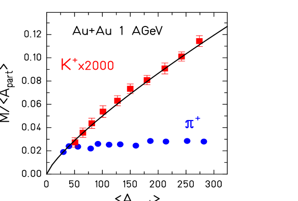
Figure 12: The yield of kaons and pions measured in Au–Au collisions at beam kinetic energy of 1 A GeV from Ref. (r57) versus centrality given by the number of participants $A_{part}$. The line represents the $A_{part}^{\alpha}$ fit[118] to experimental data

.

4.1 Central heavy ion collisions at SIS energies

The number of strange particles produced in heavy ion collisions depends on the energy and centrality of the collision. In low energy A–A collisions in the SIS/GSI energy range from 1 to 2 A$\cdot$GeV, the average number of strange particles produced in an event is of the order of $10^{-3}$. Thus, following the kinetic analysis presented in Section 4.1, a statistical description would require the canonical treatment of strangeness conservation. However, the conservation of baryon number and isospin can be treated grand canonically. Consequently, one expects a different centrality dependence of strange and non-strange particle yields. Fig. (12) shows experimental data on $K^{+}$ and $\pi^{+}$ yields divided by the number of participants $A_{\rm part}$ as a function of $A_{\rm part}$ measured[118] in Au–Au collisions at beam kinetic energy of 1 A$\cdot$GeV. The data indeed exhibit the behavior expected in the canonical statistical model: a strong increase of the $K^{+}$ yield per participant and an almost constant $\pi^{+}$ yield per participant with centrality.

In the canonical model the particle densities depend on four parameters: the chemical potentials, $\mu_{Q}$ and $\mu_{B}$, related with the GC description of the electric charge and baryon number conservation, the temperature $T$ and the volume parameter appearing through the canonical treatment of the strangeness conservation. Constraints on these variables arise from the isospin asymmetry measured by the baryon number divided by twice the charge, $B/2Q$. For an isospin symmetric system this ratio is simply 1, for Ni+Ni it is 1.04 while for Au+Au this ratio is 1.25. When considering particle multiplicity ratios we are thus left with three independent parameters. The volume parameter $V$ that is responsible for the canonical suppression, the freeze–out temperature $T$ and freeze–out baryon-chemical potential $\mu_{B}$ of the fireball.

Figure 13: Lines of a constant $\pi^{+}/{\rm proton}$ ratio in the $T$–$\mu_{B}$ plane obtained[49] in the statistical model.

Figure 14: Lines of constant deutron/proton ratio in the $T$–$\mu_{B}$ plane obtained[49] in the statistical model.

Figs. (14 - 16) show the location and sensitivity of the freeze–out parameters for different particle ratios in the $(T-\mu_{B})$ plane when varying these ratios in the range obtained at SIS energy. The deuteron to proton $d/p$ and the $\pi^{+}/p$ ratios provide a good determination of the range of thermal parameters. The $\pi^{+}/p$ curve in the $(T-\mu_{B})$ plane shows temperature saturation for a large $\mu_{B}$ that establishes the upper limit of the freeze–out temperature $T$. On the other hand, the $d/p$ ratio fixes the range of the freeze–out value for $\mu_{B}$ as it shows a steep dependence on the temperature. The $K^{+}/K^{-}$ ratio in Fig. (16) exhibits a similar behavior as $d/p$ and is also independent of the volume parameter as is evident from Eq. (45) when requiring that $S=0$.

Figure 15: Lines of a constant $K^{+}/K^{-}$ ratio in the $T$–$\mu_{B}$ plane obtained[49] in the statistical model.

Figure 16: The freeze–out parameters in the $T$–$\mu_{B}$ plane calculated[49] for a fixed value of the ratio $K^{+}/\pi^{+}=0.003$ and for different correlation volumes $V=4\pi R^{3}/3$ with $R=4,6,12$ fm and $R=\infty$.

The variation of thermal parameters with the system size is shown in Fig. (16) using as an example the $K^{+}/\pi^{+}$ ratio. For a given system size the $K^{+}/\pi^{+}$ ratio clearly determines a lower limit of the freeze–out temperature as it saturates for a large $\mu_{B}$. Changing the volume parameter $V=4/3\pi R^{3}$ implies a substantial modification of the line in the $(T-\mu_{B})$ plane calculated for a fixed value of the $K^{+}/\pi^{+}$ yields. Thus, in the canonical model, the strange to non-strange particle ratio requires an additional consideration of the range of correlation of strange particles that is quantified by the volume parameter $V$. This parameter is assumed to be related to the number of nucleons participating in A–A collisions. From a detailed analysis of experimental data from SIS up to AGS energies it was shown that $V$ can be identified[49] as the initial overlap volume of the system created in A–A collisions. Thus, it is obtained from the atomic number of the colliding nuclei and from the impact parameter by simple geometric arguments. In heavy ion collisions at SIS energies a good description of Ni–Ni and Au–Au data was obtained[49]^, when choosing $V\simeq V_{0}A_{part}/2$ with $V_{0}\simeq 7$fm³ i.e. of the same order as the volume of the nucleon.

Figure 17: The lines in the $T$–$\mu_{B}$ plane calculated[49] in the statistical model for different particle ratios obtained in central Ni–Ni collisions at 1.8 A$\cdot$GeV .

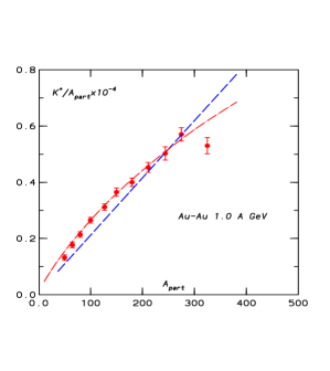
Figure 18: A comparison of the statistical model results[49] for the $K^{+}/A_{part}$ ratio with the data from Fig. (12). The dashed and dashed–dotted lines represent predictions of the statistical model without and with a small $A_{part}$ dependence of $\mu_{B}$ and $T$. For more details see text.

The comparison of the thermal model with experimental data from AGS, SPS up to RHIC energy was discussed in Section 3 and it was shown that there are common freeze–out parameters which describe simultaneously all measured particle multiplicity ratios. In order to illustrate that this is also the case in low energy heavy ion collisions we show in Fig. (18) the lines in the $(T-\mu_{B})$ plane corresponding to different particle multiplicity ratios measured[119] in Ni-Ni collisions at 1.8 $A\cdot$GeV. The experimental errors are for simplicity not shown in the figure. All lines, except the one for $\eta/\pi^{0}$, have a common crossing point around $T\sim 70$ MeV and $\mu_{B}\sim 760$ MeV. A value of $R\sim 4$ fm is needed to describe the measured $K^{+}/\pi^{+}$ ratio with the freeze–out parameters extracted from $\pi^{+}/p$ and $d/p$ ratios. This radius is compatible with that expected for a central Ni–Ni collision and was found[49] to be the same in the whole energy range from 0.8 up to 1.8 A$\cdot$GeV.

The corresponding results for a thermal description of Au-Au collisions at two different incident kinetic energies 1.0 and 1.5 $A\cdot$GeV can be found in Ref. (r31). As for Ni–Ni data, the particle ratios, $\pi^{+}/p$, $K^{+}/\pi^{+}$, $\pi^{+}/\pi^{-}$, $K^{+}/K^{-}$ and $d/p$, with exception of $\eta/\pi^{0}$, could be described with the same value of the freeze–out parameters. The temperature $T\sim 53$ MeV and $\mu_{B}\sim 822$ MeV were found in Au–Au collisions at 1.0 A$\cdot$GeV. Thus, the freeze–out temperature is obviously decreasing whereas the baryon chemical potential is an increasing function of the collision energy. A small variation of freeze–out parameters with A in central A–A collisions for the same collisions energy was also extracted from the data[49].

The observed scaling of the volume parameter that determines the canonical suppression of the strange particle phase–space with the number of participants was also found to be valid in Au–Au collisions. Here, in the most central collisions a radius of $\sim 6.2$ fm is required to reproduce the measured $K^{+}/A_{part}$ and $K^{-}/A_{part}$ yields. The larger radius value obtained for Au compared to Ni data is compatible with the larger size of Au and corresponds to $A_{part}\sim 330$ in the most central Au–Au collisions.

The importance of strangeness suppression due to canonical treatment of the conservation laws is particularly transparent in the comparison of the thermal model with the Au-Au data at 1 $A\cdot$GeV . Using the grand canonical formulation of the strangeness conservation one would get a value of $K^{+}/\pi^{+}\sim 0.04$ that overestimates the data by more than an order of magnitude. This shows that the thermal particle phase–space at SIS energies is far from the grand canonical limit and that the exact and local treatment of strangeness conservation is of crucial importance.

The multiplicity of $K^{+}$ per participant ($K^{+}/A_{part}$) was indicated in Fig. (12) to increase strongly with centrality while the corresponding ratio for pions $\pi^{+}/A_{part}$, is constant with $A_{part}$[119]. Consequently, the pion yield is proportional to the number of participants while the multiplicity of $K^{+}$ scales with $A_{part}$ as $K^{+}\sim A_{part}^{\alpha}$ with $\alpha\sim 1.8$. The canonical treatment of the strangeness conservation predicts the yield of strange particles to increase quadratically with the number of participants, see e.g. Eq. (28). In Fig. (18) the experimental data from Fig. (12) are compared with the thermal model. The parameters were chosen to reproduce the $\pi/p$ and $d/p$ ratios. The dashed-line in Fig. (18) describes the results of a thermal model under the assumption that both $T$ and $\mu_{B}$ are independent of $A_{part}$. One sees that already under this approximation the agreement of the model and the experimental data is very satisfactory as the model describes the magnitude and the centrality dependence of these data. Some differences between the model and the data seen in Fig. (18) can be accounted for when including a small variation of the freeze–out parameters with $A_{part}$. A smooth and almost linear increase of the temperature with centrality by a few MeV and a corresponding decrease of $\mu_{B}$ from very peripheral to central collisions is sufficient to get a very good description of the data. In Fig. (18) the dashed–dotted line shows thermal model results that include the variation of thermal parameters with centrality. Such a small dependence of the freeze–out temperature on impact parameter comes at first glance as a surprise since the experimental result on the apparent inverse slope parameter $T_{app}$ of particle yields as a function of $p_{t}$ in Au–Au collisions shows a strong dependence on $A_{part}$[124, 123]. This difference, however, can be accounted for by including the concept of centrality dependent transverse collective flow of the collision fireball. A detailed analysis of particle spectra in Au–Au collisions at 1 A$\cdot$GeV has shown that keeping the chemical freeze–out temperature at $53$ MeV and including collective transverse flow reproduces the transverse momentum distributions of pions, protons and kaons as well as their centrality dependence[49]. This result indicates that chemical and thermal freeze–out coincide at SIS energy.

The canonical thermal model provides a consistent description of the experimental data in the GSI/SIS energy range. The abundances of $K^{+},K^{-}$, $p,d,$ $\pi^{+}$ and $\pi^{-}$ hadrons (with the notable exception of $\eta$ and possibly $\phi$) seem to come from a common hot source and with well defined temperature, $T\approx 50,54,70$ MeV, and baryon chemical potential $\mu_{B}\approx 825,805,750$ MeV for central Ni-Ni collisions at 0.8, 1.0, 1.8 $A\cdot$GeV and correspondingly $T\approx 53$ MeV and $\mu_{B}\approx 822$ MeV for central Au-Au collisions at 1.0 $A\cdot$GeV. These temperatures are lower than the ones observed in the particle spectra but here a common explanation is possible in terms of hydrodynamic flow. The flow differentiates between particles of different mass since they acquire the same boost in velocity but very different boosts in momentum.

The common freeze–out condition for almost all particle species is very strong evidence for chemical equilibrium in low energy heavy ion collisions. A satisfactory agreement of the model and the data could be only obtained when including a canonical description of the strangeness conservation. The relevant parameter that quantifies the canonical suppression of the particle phase–space was found to be the initial volume of the collision fireball that scales with the number of projectile participants. This volume parameter describes the range of strange particle correlations and is smaller than the radius of the fireball at chemical freeze–out. In central Au–Au collisions at 1 A$\cdot$GeV the correlation radius was found to be 6.2 fm roughly corresponding to the size of Au whereas the radius required to reproduce measured particle yields is almost two times larger[49]. The appearance of two different space–like scales in the canonical description of particle production can be possibly understood from the kinetics of strangeness production. Introducing the locality of strangeness conservation in the kinetic equation (15) implies that the volume parameter in the loss terms can be different (smaller) than in the gain terms. Consequently, strange particle yields depend on two volume parameters: (i) the volume of the fireball which is also an overall normalization factor that determines the total strange and non-strange particle yields originating from the collisions fireball and (ii) the volume that parameterizes the space-like correlations of strange particles that is required to satisfy exactly the strangeness conservation. The second parameter is also related with the initial number of nucleons participating in the collision.

The apparent chemical equilibration of particle yields measured at SIS energies and the kinetic theory developed in Section 4 has recently inspired a more complete dynamical study of the problem in terms of microscopic transport models[125]^-[128]. Recently the relativistic transport model was applied[129, 130] to describe the chemical equilibration of kaon and anti-kaon at energies that are below the N–N threshold. The results of these microscopic studies indicate that $K^{+}$ can possibly appear in chemical equilibrium during the lifetime of the collision fireball. The $K^{-}$, on the other hand, approaches chemical equilibrium even at a earlier times However, it may eventually fall out of equilibrium at a later time due to the large annihilation cross sections in nuclear matter[130]. Thus, the results of transport models do not exclude chemical equilibration in low energy heavy ion collisions. The level of equilibration in these models is strongly related to the magnitude of production and absorption cross section of kaons inside the nuclear medium[131]. Although significant progress has been made in the theoretical description and understanding of in-medium kaon cross sections, the results are still far from complete. In particular, recently it was suggested that the coupling of kaons with the p-wave $\Sigma(1385)$ resonance can substantially increase the $K^{-}$ production cross section that could influence[132] the approach of kaons towards an equilibrium.

4.2 Particle production in high energy p–p collisions

The success of the statistical approach in the description of particle production in heavy ion collisions discussed in Sections 3 and 4 prompts the question if a statistical order of the secondaries is also observed in elementary collisions such as high energy p–p interactions, to which we restrict our discussion. The results of Section 4 make it clear that one should in this case apply a model that accounts for the canonical conservation of the quantum numbers. This is particularly the case for strangeness since even in very high energy p–p collisions the number of produced strange particles per event is of the order of unity. Thus, large, event by event, strange particle multiplicity fluctuations prevent the applicability of the GC approach. Whether or not the GC treatment of the baryon number and electric charge is adequate, would require a detailed study of the relative error between the canonical and the grand canonical results.

The application of the statistical model to the elementary hadron–hadron reactions was first proposed by Rolf Hagedorn[105] in order to describe the exponential shape of the $m_{t}$-spectra of produced particles in p–p collisions. Hagedorn also pointed out phenomenologically the importance of the canonical treatment of the conservation laws for rarely produced particles. The first application of the canonical model to strangeness production in p–p collisions was done by Edward Shuryak[105] in the context of ISR data. Recently a complete analysis of hadron yields in p–p as well as in $\bar{\rm p}$–p, $e^{+}e^{-}$, $\pi$–p and in ${\rm K}$–p collisions at several center-of-mass energies has been done in Refs. (r17,becalast,r41). This detailed analysis has shown that particle abundances in elementary collisions can be also described by a statistical ensemble with maximized entropy. In fact, measured yields are consistent with the model assuming the existence of equilibrated fireballs at a temperature $T\approx$160-180 MeV.

Figure 19: A comparison[133] of the p–p multiplicity data at $\sqrt{s}=27.4$ with the statistical model that accounts for the exact conservation of baryon number, electric charge, strangeness and includes the strangeness undersaturation factor $\gamma_{s}\simeq 0.51$.

The most general partition function $Z_{B,Q,S}(V,T)$ that is applied to test the chemical composition of the secondaries in elementary collisions should account for the canonical conservation of baryon number $B$, strangeness $S$, and electric charge $Q$. It can be constructed applying the projection method (see Section 4.2) for the $U_{B}(1)\times U_{S}(1)\times U_{Q}(1)$ symmetry. Following Eq. (79) one has

$$Z_{B,Q,S}(V,T)= \int_{0}^{2\pi}{{d\phi_{B}}\over{2\pi}}e^{-iB\phi_{B}}\int_{0}^{2\pi}{{d\phi_{Q}}\over{2\pi}}e^{-iQ\phi_{Q}}$$ (114)

$$\int_{0}^{2\pi}{{d\phi_{S}}\over{2\pi}}e^{-iS\phi_{S}}e^{\ln\tilde{Z}(T,V,\phi_{B},\phi_{Q},\phi_{S})},$$

where $B,Q$, and $S$ are the initial values of the quantum numbers in hadron–hadron collisions which are in p–p scattering B=Q=2 and S=0.

The generating function $\tilde{Z}$ in Eq. (114) can be obtained from the grand canonical partition function of a hadron resonance gas (3) by a Wick rotation of all appropriate chemical potentials

$$\tilde{Z}(T,V,\phi_{B},\phi_{Q},\phi_{S})=$$

$$Z^{GC}(T,V,\mu_{B}\to-i\beta\phi_{B},\mu_{Q}\to-i\beta\phi_{Q},\mu_{S}\to-i\beta\phi_{S}).$$ (115)

Different particle multiplicities and their ratios are obtained from the partition function (114) following the procedure that was described in Section 4.2.3.

Fig. (19) shows an example of the comparison of the canonical model prediction (114) with the experimental data for different particle yields obtained[133] in p–p collisions at $\sqrt{s}=27.4$–$27.6$ GeV. The agreement of the model with most of the experimental data is reasonable.

Figure 20: A comparison of the p–p multiplicity obtained at $\sqrt{s}=27.4$ with the canonical models. The open symbols represent the result of the model that accounts for $S,B$ and $Q$ being exactly conserved[133]. The filled symbols are the statistical model results with only $S$ being exact whereas $B$ and $Q$ are treated grand canonically.

Figure 21: As in Figure (21) but the filled circle are obtained in the canonical model that accounts for the strangeness undersaturation to be controlled by the correlation volume, $V_{p}=4\pi R_{p}^{3}/3$ with $R_{p}\simeq 1.1$ fm instead of $\gamma_{s}$.

However, the yields of the resonances like $\Delta^{0},\rho^{0}$ and $\phi$ can differ by a few standard deviations from the data leading to rather large reduce $\chi^{2}$ values of $\simeq 5$.

The agreement of the model with the strange particle yields could only be, however, achieved in Ref. (r41) when introducing[105, 133] an additional parameter $\gamma_{s}$ into the canonical partition function (114). This parameter suppresses a thermal phase–space of particles composed of $n_{s}$ strange or antistrange quarks by a factor $(\gamma_{s})^{n_{s}}$. In p–p and $\bar{\rm p}$–p collisions and in a very broad energy range from $\sqrt{s}\sim 20$ up to $\sqrt{s}\sim 900$ GeV the same value of $\gamma_{s}\simeq 0.51$ was needed[133] to reproduce the measured strange particle yields.

In high energy p–p collisions the canonical effects due to the baryon number and isospin conservation are expected to be small. Fig. (21) shows the comparison of p–p data with the canonical model that accounts for only strangeness being conserved exactly. The baryon number and electric charge conservation are treated in the GC ensemble, thus are controlled by chemical potentials. A satisfactory description of experimental data with $\mu_{B}\sim 195$ MeV, $\mu_{Q}\sim 30$ MeV, $T\sim 165$ MeV and $\gamma_{s}\sim 0.53$ seen in Fig. (21) shows that canonical effects related with charge and baryon number conservation are indeed small[134]. This is, however, not the case in $\bar{\rm p}$–p and $e^{+}e^{-}$ collisions since the initial values of $B=Q=0$ are there obviously too small to use a GC approximation.

The experimental data shown in Fig. (19) can be also described in terms of the canonical model that was successfully applied in low energy heavy ion collisions (see Section 5.1). There, instead of the strangeness undersaturation factor $\gamma_{s}$, space-like correlations of strange particles were introduced. Consequently, there were two volume parameters that determined particle yields: (i) the volume of the fireball and, (ii) the correlation volume. Fig. (21) shows that choosing the correlation volume $V_{p}=4\pi R_{p}^{3}/3$ and $R_{p}\sim 1.1-1.2$ fm the p–p data are well reproduced with the exception of $\phi$. The $\phi$-meson is not canonically suppressed because it only carries zero strangeness. Taking the correlation volume instead of $\gamma_{s}$ gives a deviation of the measured $\phi$ abundance from a thermal fit of $12\sigma$, thus increasing even more the already large deviation of $4\sigma$ seen in Fig. (19). The canonical model that introduces a $\gamma_{s}\sim 0.5$ factor[133] is obviously better reproducing the yields of hidden strange particles obtained in elementary collisions.

The value of $\gamma_{s}$ extracted from p–p data is smaller than required[40] in central Pb–Pb at 160 A$\cdot$GeV where for fully integrated yields $\gamma_{s}=0.75\pm 0.05$ was fitted. This result shows that the undersaturation of strangeness in p–p and A–A collisions differs by almost $50\%$. This difference alone already indicates[9] that strangeness in A–A is enhanced relative to p–p collisions.

The temperature parameter extracted from particle yields in high energy elementary collisions is at first glance surprisingly compatible with the chemical freeze–out temperature extracted from heavy ion data[40, 133]. At SPS and RHIC energies, $T$ can be considered as a measure of thermal excitations of a non–perturbative QCD vacuum due to the particle scattering. Thus, $T$ should be mostly correlated with the collision energy and not with the system size. The charge chemical potential, however, due to the isospin asymmetry, differers substantially in p–p and A–A collisions. In Pb–Pb collisions at the SPS the $\mu_{Q}\sim-7$ MeV[38] whereas in p–p at $\sqrt{s}\simeq 27$ the $\mu_{Q}\sim 35$ MeV is required.

4.2.1 Statistical hadronization and string dynamics in p–p collisions

The apparent agreement of the canonical statistical model with experimental data on particle production in elementary collisions leads to the interpretation that hadronization in particle collisions is a statistical process. This result is difficult to reconcile with the popular picture that hadron production in hadron–hadron collisions is due to the decay of color flux tubes[135], a model that has explained many dynamical features of these collisions. In the following we address the question, how one can possibly distinguish the string hadronization via the break up of a color flux tube from the statistical hadronization. We argue following Ref. (markus) that the $\overline{\Omega}/\Omega=\Omega^{+}/\Omega^{-}$ ratio in elementary proton–proton collisions is a sensitive probe to differentiate possibly these two scenarios.

Color flux tubes, called strings, connect two SU(3) color charges [ $3$ ] and [ $\overline{3}$ ] with a linear confining potential. If the excitation energy of the string is high enough it is allowed to decay via the Schwinger mechanism[137], i.e. the rate of newly produced quarks is given by:

$$\frac{{\rm d}N_{\kappa}}{{\rm d}p_{\perp}}\sim{\rm\exp}\left[-\pi m_{\perp}^{2}/\kappa\right],$$ (116)

where $\kappa$ is the string tension and $m_{\perp}=\sqrt{p_{\perp}^{2}+m^{2}}$ is the transverse mass of the produced quark with mass $m$.

However, specific string models may differ in their philosophy and the types of strings that are created:

• In UrQMD[125] the projectile and target protons become excited objects due to the momentum transfer in the interaction. The resulting strings, with at most two strings being formed, are of the diquark–quark type.

• In NeXuS[126], the p–p interaction is described in terms of pomeron exchanges or ladder diagrams. Both hard and soft interactions take place in parallel. Energy is equally shared between all cut pomerons and the remnants. The endpoints of the cut pomerons (i.e. the endpoints of the strings) may be valence quarks, sea quarks or antiquarks.

• In PYTHIA[127], a scheme similar to that in UrQMD is employed. However, hard interactions may create additional strings from scattered gluons and sea quarks. Most strings are also of a diquark–quark form.

Fig. (22 -left) depicts the antibaryon to baryon ratio at midrapidity in proton–proton interactions at 160 GeV. The results of the calculations by NeXuS, UrQMD and PYTHIA are included in this figure[136]. In all these models, the $\overline{B}/B$ ratio increases strongly with the strangeness content of the baryon. For strangeness $|s|=3$ the ratio significantly exceeds the unity. In UrQMD and PYTHIA the hadronization of the diquark–quark strings leads directly to the overpopulation of $\overline{\Omega}$. In NeXuS, however, the imbalance of quarks and anti quarks in the initial state leads to the formation of $q_{\rm val}-\overline{s}_{\rm sea}$ strings (the $s_{\rm val}-\overline{q}_{\rm sea}$ string is not possible). These strings result then in the overpopulation of $\overline{\Omega}^{,}$s.

In order to understand the large $\overline{\Omega}/\Omega$ values predicted by string models we include in Fig. (23), the color flux tube break-up mechanism.

Fig. (23) shows the fragmentation of the color field into quark-antiquark pairs, which then coalesce into hadrons. While in large strings $\Omega^{,}$s and $\overline{\Omega}^{,}$s are produced in equal abundance (a), low-mass strings in UrQMD suppress $\Omega$ production at the string ends (b), while in NeXuS $\overline{\Omega}$^,s are enhanced (c). Thus, the microscopic method of hadronization leads to a strong imbalance in the $\overline{\Omega}/\Omega$ ratio in low-mass strings.

figure=rfig20.ps,width=3.2in

Figure 22: The left hand figure: the anti baryon to baryon ratio at $|y-y_{\rm cm}|<1$ in p–p interactions at 160 GeV as given by PYTHIA, NeXuS and UrQMD. The right hand figure: the anti baryon to baryon ratio for the same reaction as given by the statistical models. Stars depict preliminary NA49 data for the $\overline{B}/B$ ratio at midrapidity.

In Fig. (22) the string model results are compared with the predictions of two statistical models (SM)[135] and the preliminary experimental data obtained[138] by the NA49 Collaboration. The main difference between these models is the implementation of baryon number and electric charge conservation and the way an additional strangeness suppression is introduced. In model (i) the calculation[56] is a full canonical one with fixed baryon number, strangeness and electric charge identical to those of the initial state. An extra strangeness suppression is introduced to reproduce the experimental multiplicities. This is done by considering the number of newly produced $\langle s\overline{s}\rangle$ pairs as an additional charge to be found in the final hadrons. The $s\overline{s}$ pairs fluctuate according to a Poisson distribution and their mean number is considered as a free parameter to be fitted[56]. The parameters used for the prediction of the $\Omega^{+}/\Omega^{-}$ ratio ($T$, the global volume $V$ sum of single cluster volumes and $\langle s\overline{s}\rangle$) have been obtained by a fit to preliminary NA49 p–p data[138] yielding $T=183.7\pm 6.7$ MeV, $VT^{3}=6.49\pm 1.33$ and $\langle s\overline{s}\rangle=0.405\pm 0.026$ with a $\chi^{2}/{\rm dof}=11.7/9$. It must be pointed out that the $\Omega^{+}/\Omega^{-}$ ratio is actually independent of the $\langle s\overline{s}\rangle$ parameter and only depends on $T$ and $V$.

figure=rfig21.ps,width=3in

Figure 23: Fragmentation of a color field into quarks and hadrons. While in large strings $\Omega^{,}$s and $\overline{\Omega}^{,}$s are produced in an equal abundance (a), small di^,quark strings suppress $\Omega^{,}$s at the string ends (b), sea-$\overline{s}$ quarks enhance $\overline{\Omega}^{,}$s (c).

In model (ii) the conservation of the baryon number and electric charge is approximated by using the GC ensemble. The strangeness conservation is, however, implemented on the canonical level following the procedure that accounts for strong correlations of produced strange particles. In p–p collisions the strangeness is assumed not to be distributed in the whole volume of the fireball but to be locally strongly correlated. A correlation volume parameter $V_{0}=4\pi R_{0}^{3}/3$ is introduced, where $R_{0}\sim 1$ fm is a typical scale of QCD interactions. The temperature $T\simeq 158$ MeV and $\mu_{B}\simeq 238$ MeV were taken as obtained[40] from the SM analysis of a full phase-space Pb–Pb data of NA49 Collaboration. The volume of the fireball $V\sim 17$ fm³ and the charge chemical potential in p–p was then found to reproduce the average charge and baryon number in the initial state.

The predictions of the statistical models are shown in Fig. (22 -right). In these approaches the $\overline{B}/B$ ratio is seen to exhibit a significantly weaker increase with the strangeness content of the baryon than that expected in the string fragmentation models. For comparison, both figures include preliminary data on the $\overline{B}/B$ ratios obtained[138] at midrapidity by the NA49 Collaboration. Note that the predictions of the statistical models in Fig. (22) refer to full phase-space particle yields whilst measurements of $\overline{B}/B$ ratios in p–p collisions have been performed at midrapidity, where they are expected to be the largest. Therefore, sizeable deviations of the model results from the data seen in Fig. (22) are to be expected. However, admitting the applicability of SM for midrapidity one reproduces[141] the experimental data quite well.

In macroscopic string models the $\overline{\Omega}/\Omega$ ratio depends in a strongly non-linear fashion on the mass (energy) of the fragmenting string. All these models predict a strong enhancement of $\overline{\Omega}$ production at low energies, while for large string masses the ratio approaches the value of $\overline{\Omega}/\Omega=1$ (which should be reached in the limit of an infinitely long color flux tube).

Statistical models, on the other hand, are not able to yield a ratio of $\overline{\Omega}/\Omega>1$. This can be easily understood in the GC formalism, where the $\overline{B}/B$ ratio is very sensitive to the baryon chemical potential $\mu_{B}$. For finite baryon densities and including 100$\%$ feeding from resonances, the $\overline{B}/B$ ratio will always be $<1$ and only in the limit of $\mu_{B}=0$ may $\overline{\Omega}/\Omega=1$ be approached. These features survive in the canonical framework, where the GC fugacities are replaced by the ratios of partition functions[105, 106, 107].

From the above discussion and from Fig. (22) it is thus clear that within the fragmenting color flux tube models the $\overline{\Omega}/\Omega$ ratio is significantly above the unity. This is in strong contrast to statistical model results, that always imply that $\overline{B}/B$ ratios are below or equal to a unity in proton–proton reactions. Since this observable is accessible to NA49 measurements at the SPS it can provide an excellent test to distinguish the statistical model hadronization scenario from that of a microscopic color-flux tube dynamics.

We have to point out, however, that the classical string models considered above do not account for the so called string junction mechanism that allows for diffusion of baryon number towards midrapidity. This mechanism, recently included[139] in Dual Parton Model, was shown to be very important for (multi)strange baryon and antibaryon production. Thus, it would be of importance to study the energy dependence of $\bar{B}/B$ ratio in p–p collisions in terms of the model that includes this baryon number transport.

4.3 Heavy quark production

Charm quarks are heavy ($m_{c}\gg T_{c}$) thus, thermal production of charm quarks and charmed hadrons is strongly suppressed in ultra-relativistic heavy ion collisions[142]. The situation has been recently discussed[75, 76] with the conclusion that, compared to direct hard production, thermal production of charm quarks can be neglected at SPS energies and is small even at LHC energy. However, these investigations led to a new scenario for the production of hadrons which contain charm quarks in which production of heavy quarks through hard collisions is combined with a statistical procedure to produce open and hidden charm hadrons at hadronization. This idea of statistical hadronization of charm quarks[75, 76] has sparked an intense activity in this field[143, 144]. Initial interest focussed on the available SPS data on $J/\psi$ production and their interpretation in terms of a conventional statistical model[145]. As we show below, these data can be well described, but only assuming a charm cross section which is enhanced compared to predictions within the framework of perturbative QCD. However, the largest differences between results from the statistical coalescence scenario (or a similar[146] model) and more conventional models are expected at collider energies. For example, in the Satz-Matsui approach[28], one would expect very strong suppression compared to direct production of $J/\psi$ mesons (up to a factor[147] of 20) for central Au-Au collision at RHIC energy. In the present approach this suppression is overcome by statistical recombination of $J/\psi$ mesons from the same or different $c\bar{c}$ pairs, so that much larger yields are expected. We therefore focus in this section on predictions for open and hidden charm mesons at RHIC and LHC energy, with emphasis on the centrality dependence of rapidity densities.

4.3.1 Statistical Recombination Model

In this model it is assumed that all charm quarks are produced in primary hard collisions and (thermally) equilibrate in the quark-gluon plasma (QGP); in particular, no $J/\psi$ is preformed in QGP (complete screening) and there is no thermal production of charm quarks. For a description of the hadronization of the c and $\bar{\rm c}$ quarks, i.e. for the determination of the relative yields of charmonia, and charmed mesons and baryons, we employ the statistical model, with parameters as determined by the analysis of all other hadron yields[175]. The picture we have in mind is that all hadrons form within a narrow time range at or close to the phase boundary. All charmed hadrons (open and hidden) are formed at freeze-out (at SPS and beyond, freeze-out is at the phase boundary[175]) according to the statistical laws.

Another interesting point concerns the $\psi^{{}^{\prime}}$/(J/$\psi)$ ratio. As is well known, this ratio is, in hadron-proton and p-nucleus collisions, close to 12 %, independent[152] of collision system, energy, transverse momentum etc.. In the thermal model, the ratio is 3.7 %, including feeding of the J/$\psi$ from heavier charmonium states. A temperature of about 280 MeV would be necessary to explain the ratio found in pp and p-nucleus collisions in a thermal approach. Clearly, J/$\psi$ and $\psi^{{}^{\prime}}$ production in pp and p-nucleus collisions are manifestly non-thermal. This was previously realized in Refs. (gerschel,shuryak). Similar considerations apply for the $\chi$ states. In fact, feeding from $\chi_{1}$ to J/$\psi$ is less than 3 % if the production ratios are thermal.

The experimental situation concerning the evolution with participant number of the $\psi^{{}^{\prime}}$/(J/$\psi)$ ratio in nucleus-nucleus collisions, multiplied with the respective branching into muon pairs, is presented in Fig. (24). The data are from the NA38/50 collaboration[155, 156, 157, 158]. With increasing N_part the $\psi^{{}^{\prime}}$/(J/$\psi)$ ratio drops first rapidly (away from the value in pp collisions) but seems to saturate for high N_part values at a level very close to the thermal model prediction, both for S+U and Pb–Pb collisions

Figure 24: Comparison of the dependence of the measured $\psi^{{}^{\prime}}$/(J/$\psi)$ ratio on the number of participating nucleons with the prediction of the thermal model. The data of NA38 and NA50 Collaborations are from Refs. (na38_1,na50_4,na50_5,na38_2). See text and Refs. (r611,r612) for more details.

Taking this into account we note that predictions of the model should only be trusted from about N${}_{part}>150$ on, where also the $\psi^{\prime}/(J/\psi)$ ratio is close to the thermal value for Pb–Pb data. In our approach, ratios for all higher charmonia states including the $\chi_{c}$ should approach the thermal value from N${}_{part}>150$ on, implying that for those N_part values feeding to J/$\psi$ should be small. In this picture, there should thus not be different “thresholds” for the disappearance of different charmonia.

The total number of open charm hadrons expected in a purely thermal approach , $N_{oc}^{th}$, is then readjusted to the number of directly produced $c\bar{c}$ pairs, $N_{c\bar{c}}^{dir}$ as (neglecting charmonia): $N_{c\bar{c}}^{dir}=\frac{1}{2}g_{c}N_{oc}^{th}{I_{1}(g_{c}N_{oc}^{th})}/{I_{0}(g_{c}N_{oc}^{th})}$, from which the charm enhancement factor $g_{c}$ is extracted. Here, $I_{n}$ are modified Bessel functions. Note that we use here the canonical approach as, depending on beam energy, the number of charm quark pairs maybe smaller than 1. The grand-canonical limit will likely only be reached at LHC energy. For a detailed study of the transition from the canonical to the grand-canonical regime see Section 3.2 and Ref. (r612). The yield of a given species $X$ is then determined by $N_{X}=g_{c}N_{X}^{th}{I_{1}(g_{c}N_{oc}^{th})}/{I_{0}(g_{c}N_{oc}^{th})}$ for open charm mesons and hyperons and $N_{X}=g_{c}^{2}N_{X}^{th}$ for charmonia (see Refs. (r611,r612) for more details).

The inputs for the above procedure are: i) the total charged particles yields (or rapidity densities), which are taken from experiments at SPS[185, 159] and RHIC[184] and extrapolated for LHC; and ii) $N_{c\bar{c}}^{dir}$, which is taken from next-to-leading order (NLO) perturbative QCD (pQCD) calculations for pp[160] (the yield from MRST HO parton distributions was used here) and scaled to AA via the nuclear overlap function. A constant temperature of 170 MeV and the baryonic chemical potential $\mu_{b}$ according to the parameterization $\mu_{b}$(MeV)=$1270/(1+\sqrt{s_{NN}}/4.3$ have been used for the calculations[53].

4.3.2 Results

We first compare predictions[148, 149] of the model to 4$\pi$-integrated $J/\psi$ data[161] at the SPS from NA50 Collaboration replotted as outlined in Ref. (r612). In Fig. (25) we present the model results for two values of $N_{c\bar{c}}^{dir}$: from NLO calculations[160] (dashed–line) and scaled up by a factor of 2.8 (continuous line). The dashed–dotted line in Fig. (25) is obtained with the NLO cross section for charm production scaled–up by a factor 1.6, which is the ratio of the open charm cross section estimated[153] by NA50 for p–p collisions at 450 GeV/c and the NLO values from Ref. (andronic1). For this case the $N_{part}$ scaling is not the overlap function, but is taken according to measured[153] dimuon enhancement as a function of $N_{part}$.

The results of Fig. (25) indicate that the observed centrality dependence of $J/\psi$ for $100<N_{part}<$350 is well reproduced by the statistical model using the NLO cross sections for charm production scaled by the nuclear overlap function. However, to explain the overall magnitude of the data a $N_{c\bar{c}}^{dir}$ increase by a factor of 2.8 compared to NLO calculations is needed. The drop of the $J/\psi$ yield per participant observed in the data for $N_{part}>$350 ( see Fig. (25)) is currently understood[150] in terms of energy density fluctuations for a given overlap geometry.

We mention in this context that the observed enhancement of the dimuon yield at intermediate masses has been interpreted[163] by NA50 as possible indication for an anomalous increase in the charm cross section. We note, however, that other plausible explanations[13, 16] exist of the observed enhancement in terms of thermal radiation.

Figure 25: The centrality dependence of $J/\psi$ production at SPS. Model predictions are compared to 4$\pi$-integrated NA50 data[161, 162]. Two curves for the model correspond to values of $N_{c\bar{c}}^{dir}\sim 0.137$ from NLO calculations[160] (dashed line) and scaled up by a factor of 2.8 (continuous line). The dashed–dotted curve is obtained when considering the possible NA50 $N_{part}$–dependent charm enhancement[163] over their extracted[153] p–p cross section (see text).

We turn now to discuss model predictions for collider energies. For comparison we include in this study also results at SPS energy. The input parameters for these calculations for central collisions ($N_{part}$=350) are presented in Table 4.3.2. Notice that from now on we focus on rapidity densities, which are the relevant observables at the colliders. The results are compiled in Table 4.3.2 for a selection of hadrons with open and hidden charm. All predicted yields increase strongly with energy, reflecting the increasing charm cross section and the concomitant importance of statistical recombination. Also ratios of open charm hadrons evolve with increasing energy, reflecting the corresponding decrease in charm chemical potential.

Input parameters for model calculations at SPS, RHIC and LHC.            $\sqrt{s_{NN}}$ (GeV)            17.3            200            5500            $T$ (MeV)            170            170            170            $\mu_{b}$ (MeV)            253            27            1            $\mathrm{d}N_{ch}/\mathrm{d}y$            430            730            2000            $V_{\Delta y=1}$ (fm³)            861            1663            4564            $\mathrm{d}N_{c\bar{c}}^{dir}/\mathrm{d}y$            0.064            1.92            16.8            $g_{c}$            1.86            8.33            23.2 [Source] A. Andronic et al. from Ref. (andronic).

Results of model calculations at SPS, RHIC and LHC for $N_{part}$=350.           $\sqrt{s_{NN}}$ (GeV)          17.3          200          5500           $\mathrm{d}N_{\mathrm{D}^{+}}/\mathrm{d}y$          0.010          0.404          3.56           $\mathrm{d}N_{\mathrm{D}^{-}}/\mathrm{d}y$          0.016          0.420          3.53           $\mathrm{d}N_{\mathrm{D}^{0}}/\mathrm{d}y$          0.022          0.89          7.8           $\mathrm{d}N_{\Lambda_{c}}/\mathrm{d}y$          0.014          0.153          1.16           $\mathrm{d}N_{J/\psi}/\mathrm{d}y$          2.55$\cdot$10^-4          0.011          0.226           $\mathrm{d}N_{\psi^{\prime}}/\mathrm{d}y$          0.95$\cdot$10^-5          3.97$\cdot$10^-4          8.46$\cdot$10^-3 [Source] A. Andronic et al. from Ref. (andronic).

Figure 26: Centrality dependence of $J/\psi$ (upper figure) and of D+ (lower figure) rapidity density at SPS, RHIC and LHC energies.

Predictions for the centrality dependence of $J/\psi$ production are presented in Fig. (26). In addition to the dramatic change in magnitude (note the scale-up by factors of 10 and 100 for RHIC and SPS energy, respectively) the results exhibit a striking change in centrality dependence, reflecting the transition from a canonical to a grand-canonical regime (see Ref. (r612) for more details). The preliminary PHENIX results on $J/\psi$ production at RHIC[165] agree, within the still large error bars, with our predictions. A stringent test of the present model can only be made when high statistics $J/\psi$ data are available. Another important issue in this respect is the accuracy of the charm cross section, for which so far only indirect measurements are available[166]. In any case, very large suppression factors as predicted, e.g., by Ref. (vogt99) seem not supported by the data. In Fig. (26) we present the predicted centrality dependence of charged D⁺-meson production for the three energies. The expected approximate scaling of the ratio D⁺/$N_{part}$ like $N_{part}^{1/3}$ (dashed lines in lower Fig. (26)) is only roughly fulfilled due to departures of the nuclear overlap function from the simple $N_{part}^{4/3}$ dependence.

4.3.3 Charmonium Production from Secondary Collisions at LHC Energy

Another possibility to produce charmonium states is due to reactions among D mesons in the hadronic and mixed phase of the collision. This has been investigated in Refs. (krpbm,ko). As demonstrated there, this mechanism does not lead to appreciable charmonium production at SPS and RHIC energies. However, the large number of $c\bar{c}$ pairs and consequently $D$,$\bar{D}$ mesons produced in Pb-Pb collisions at LHC energy can lead to an additional production of charmonium bound states due to reactions such as: $D\bar{D^{*}}+D^{*}\bar{D}+D^{*}\bar{D^{*}}\to J/\psi+\pi$ and $D^{*}\bar{D^{*}}+D\bar{D}\to J/\psi+\rho$. These processes were studied within a kinetic model taking into account the space-time evolution of a longitudinally and transversely expanding medium. The results[142] demonstrate that secondary charmonium production appears almost entirely during the mixed phase and is very sensitive to the charmonium dissociation cross section with co-moving hadrons. Within the most likely scenario for the dissociation cross section of the $J/\psi$ mesons their regeneration in the hadronic medium will be negligible, even at LHC energy. Secondary production of $\psi^{,}$ mesons however, due to their large cross section above the threshold, can substantially exceed the primary yield.

4.3.4 Conclusions on Heavy Quark Production

We have demonstrated that the statistical coalescence approach yields a good description of the measured centrality dependence of $J/\psi$ production at SPS energy, albeit with a charm cross section increased by a factor of 2.8 compared to current NLO calculation. Rapidity densities for open and hidden charm mesons are predicted to increase strongly with energy, with striking changes in centrality dependence. First RHIC data on $J/\psi$ production support the current predictions, although the errors are too large to make firm conclusions. For LHC energies we predict cross sections for charm production in central Pb-Pb collisions significantly exceeding the values predicted by scaling results for N-N collisions with the nuclear thickness function. The statistical coalescence implies travel of charm quarks over significant distances in QGP. If the model predictions will describe consistently precision data then J/$\psi$ enhancement (rather than suppression) would be a clear signal for the presence of a deconfined phase.

Regeneration of charmonia in the mixed and hadronic phase has also been studied. For J/$\psi$ mesons this will likely only be a small effect, even at LHC energy. However, secondary production of $\psi^{,}$ mesons may be significant at LHC energy.

5 Unified conditions of particle freeze–out in heavy ion collisions

A detailed analysis of experimental data in heavy ion collisions from SIS through AGS, SPS up to RHIC energy discussed in Section 3 and 5 makes it clear that the canonical or grand canonical statistical model reproduces most of the measured hadron yields.

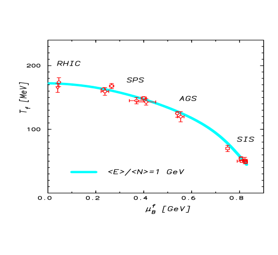
Figure 27: A compilation of chemical freeze–out parameters appropriate for A–A collisions at different energies: SIS results are from Ref. (r31), AGS from Ref. (r14), SPS at 40 A$\cdot$GeV from Refs. (r15,r16,r17,r80), SPS at 160 A$\cdot$GeV from Refs. (r12,r13,r14), and RHIC from Refs. (r10,r53,r54). The full line represents the phenomenological condition of a chemical freeze–out at the fixed energy/particle $\simeq 1.0$ GeV.[34]

Figure (27) is a compilation of chemical freeze–out parameters that are required to reproduce the measured particle yields in central A–A collisions at SIS, AGS, SPS and RHIC energy. The GSI/SIS results have the lowest freeze–out temperature and the highest baryon chemical potential. As the beam energy increases a clear shift towards higher $T$ and lower $\mu_{B}$ occurs. There is a common feature to all these points, namely that the average energy $\langle E\rangle$ per average number of hadrons $\langle N\rangle$ is approximately 1 GeV. A chemical freeze–out in A–A collisions is thus reached[34] when the energy per particle $\langle E\rangle$/$\langle N\rangle$ drops below 1 GeV at all collision energies.

In cold nuclear matter the $\langle E\rangle$/$\langle N\rangle$ is approximately determined by the nucleon mass. For thermally excited nuclear matter, in the non–relativistic approximation

$${{\langle E\rangle}\over{\langle N\rangle}}\simeq\langle m\rangle+{3\over 2}T.$$ (117)

with $\langle m\rangle$ being the thermal average mass in the collisions fireball. This result makes it clear why at SIS the energy/particle at chemical freeze–out is of the order of 1 GeV since $T\simeq 53$ MeV. At SPS and RHIC energy the leading particles in the final state (at thermal freeze–out) are pions. However, at chemical freeze–out most of the pions are still hidden in the mesonic and baryonic resonances. Thus, here the average thermal mass is larger than the pion mass and corresponds approximately to the $\rho$–meson mass. Consequently, since $\langle m\rangle>>T$, Eq. (117) can be still used to justify approximately that $\langle E\rangle/\langle N\rangle\simeq 1$ GeV at the SPS. Actually, this argument holds, to a large extent, in the whole energy range from SIS up to RHIC energy.

The physical origin of the phenomenological freeze–out condition of fixed energy/particle would require further dynamical justification and interpretation. Recently, this question has been investigated in central Pb–Pb collisions at the SPS in terms of the Ultra–relativistic Quantum Molecular Dynamics model (UrQMD)[169, 170]. A detailed study has shown that there is a clear correlation between the chemical break–up in terms of inelastic scattering rates and the rapid decrease in energy per particle. If $\langle E\rangle/\langle N\rangle$ approaches the value of 1 GeV the inelastic scattering rates drop substantially and further evolution is due to elastic and pseudo-elastic collisions that preserved the chemical composition of the collision fireball. Following the above UrQMD results and the previous suggestions[171] one could consider the phenomenological chemical freeze–out of $\langle E\rangle/\langle N\rangle\simeq 1$ GeV as the condition of inelasticity in heavy ion collisions.

Unified freeze–out conditions were also considered[172] in the context of hydrodynamical models for particle production and evolution in heavy ion collisions. There, it was suggested, that the condition for chemical freeze–out, $\langle E\rangle/\langle N\rangle\simeq 1$ GeV, selects the softest point of the equation of state, namely the point where the ratio of the thermodynamical pressure $P$ to the energy density $\epsilon$ has a minimum. The considerations were essentially based on the proposed[173] mixed phase model that seems to be consistent with the available QCD lattice data. The quantity $P/\varepsilon$ is closely related to the square of the velocity of sound and characterizes the expansion speed [174] of the reaction zone. Thus, the system lives for the longest time around the softest point that allows to reach the chemical equilibrium of its constituents. The above interpretation, however, crucially depends on the type of the equation of state used in the model.

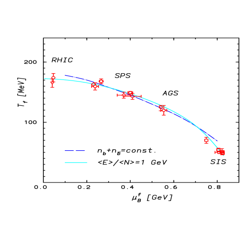
Figure 28: The broken line describes the chemical freeze–out conditions of fixed total density of baryons plus antibaryons, $n_{b}+n_{\bar{b}}=0.12/$fm³ from Ref. (r31). The full line represents the condition of the fixed energy/particle $\simeq 1.0$ GeV from Fig. (27). The freeze–out points are as in Fig. (27).

Chemical freeze–out in heavy ion collisions can also be determined[71, 187] by the condition of fixed density of the total number of baryons plus antibaryons. As it is seen in Fig. (28), within statistical uncertainties on the freeze–out parameters the above condition provides a good description of experimental data from the top AGS up to RHIC energy. However, in the energy range from SIS to AGS it slightly overestimates the freeze–out temperature for a given chemical potential. Consequently, e.g. the yield of the strange/non-strange particle ratios obtained at SIS turns out to be too large. The freeze–out conditions determined by the extensive thermodynamical observables are in addition very sensitive to the size and the model that describes repulsive interactions between hadronic constituents.

The condition of fixed $\langle E\rangle/\langle N\rangle\simeq 1$ GeV, is very insensitive to repulsive interactions. Independently on how the repulsive interactions are implemented, that is through a mean field potential[176], an effective hard core[58] or a thermodynamically consistent implementation [38, 82], the freeze–out line in Fig. (27) is hardly modified. However, the energy per particle is being sensitive to the composition of the collision fireball. Considering heavy fragments like e.g. the He or Li as being the constituents of a thermal fireball would change the line shown in Fig. (27). In general these fragments would make the line steeper below the AGS energy. This is an open question whether at the SIS energy, the multiplicity and the spectra of such composite objects are of thermal origin and can be reproduced with the same parameters as all other hadrons. For higher energies beyond AGS, however, the above is not excluded as discussed in Section 3.04 and in Ref.  (r80).

For the phenomenological determination of freeze–out parameters for different collision energies we use in the following the requirement $\langle E\rangle/\langle N\rangle\simeq 1$ GeV.

5.1 Chemical freeze–out and the QCD phase boundary

The chemical freeze–out temperature, found from a thermal analysis[38, 40, 35] of experimental data in Pb–Pb collisions at the SPS and in Au–Au collisions at RHIC energy is remarkably consistent, within errors, with the critical temperature $T_{c}\simeq 173\pm 8$ MeV obtained[77] from lattice Monte-Carlo simulations of QCD at a vanishing net baryon density. Thus, the observed hadrons seem to be originating from a deconfined medium and the chemical composition of the system is most likely to be established during hadronization of the quark-gluon plasma[6, 7, 9]. The observed coincidence of chemical and critical conditions in the QCD medium at the SPS and RHIC energy open the question if this property is also valid in heavy ion collisions at lower collision energies where the statistical order of the secondaries is phenomenologically well established.

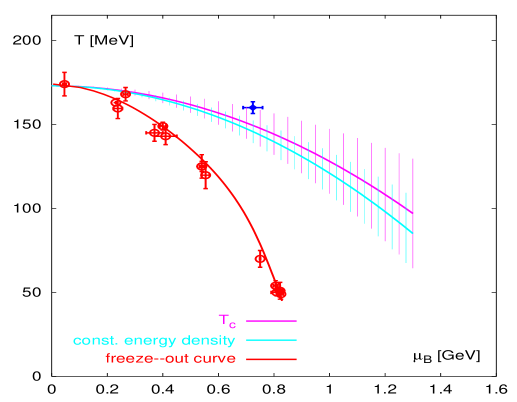
Figure 29: A Comparison of the chemical freeze–out curve from Fig. (27) with the phase boundary line. The upper thin line represents the LGT results obtained in Ref. (r81) and the lower thin line describes the conditions of constant energy density that was fixed at $\mu=0$. The upper point with crossed error bars denotes the end-point of the crossover transition from Ref. (r82).

Recently, first attempts have been made to extent lattice calculations into the region of finite $\mu_{B}$. This provided an estimate[177, 178] of the location of the phase boundary at finite baryon density. The generic problem of the Monte-Carlo simulation of QCD with the finite chemical potential, related with a complex structure of the fermionic determinant, was partly overcome. The reweighting method, in which the physical observables at finite $\mu_{B}$ are computed by simulating the theory at vanishing $\mu_{B}$[178] was successfully applied and first results on the phase boundary were obtained[178]. The region of applicability of this approach and uncertainties on the results due to a small lattice size and large strange quark mass are still, however, not well established. Another efficient method, at least for low baryon density, is based on the Taylor expansion in $\mu_{B}$ of any physical observable[177]. The coefficients of the series are calculated at vanishing $\mu_{B}$, and thus could be obtained using a standard Monte-Carlo method. This procedure was recently applied to get a series expansion of the critical temperature in terms of the critical $\mu_{B}$[177].

Fig. (29) shows the results on the position of the phase boundary that were obtained using the methods indicated above together with the freeze–out curve from Fig. (27). The upper thin-line represents an extrapolation of the leading, $(\mu_{B})_{c}^{2}$ order, term in the Taylor expansion of $T_{c}$ to a larger values of the chemical potential[177]. It is interesting to note that, within statistical uncertainties, the energy density along this line is almost constant and corresponds to $\epsilon_{c}\sim 0.6$GeV/fm³ (thin lower line in Fig. (29)), that is the same value as found on the lattice at $\mu_{B}=0$. It is thus, conceivable that the critical $(\mu_{B}^{c}-T_{c})$ surface is determined by the condition of fixed energy density. This can be also argued phenomenologically. The transition from a confined to deconfined phase could appear if the particle (like in percolation models) or energy density is so large that hadrons start to overlap. It should not be important if this density is achieved by heating or compressing the nuclear matter. Thus, since the percolation type argument[179] is well describing critical conditions at $\mu_{B}=0$ it could be also valid at finite $\mu_{B}$.

Fig. (29) shows that the chemical freeze–out points at SPS and RHIC energy are indeed lying on the phase boundary. The results of SPS at 40 A$\cdot$GeV and top AGS are already below the boundary line. However, it is not excluded that also at these lower energies the collision fireball in the initial state appears in the deconfined phase. The initial energy density expected at AGS is of the order of 1 GeV/fm³ (see Section 1.1) thus, it is larger than the critical energy density along the boundary line in Fig. (29).

The canonical suppression effects for strangeness production, were shown to be negligible already at the top AGS energies. Here, strangeness was uncorrelated and well described by the GC approach. It is quite possible that the asymptotic GC formulation and the maximal thermal phase space for strangeness is achieved if in the initial state the system was created in a deconfined, QGP phase. The abundant production of strangeness in the QGP[31] together with a long range correlations during a non-perturbative hadronization results in strangeness population that maximizes the entropy in the GC limit. In this context the energy range between SIS and 40 A$\cdot$GeV is of particular interest and it is expected to be covered by the planned[180] for the future heavy ion experiments at GSI.

6 Particle yields and their energy dependence

The hadronic composition in the final state obtained in heavy ion collisions is determined solely by an energy per hadron to be approximately 1 GeV per hadron in the rest frame of the system under consideration. This phenomenological freeze–out condition provides the relation between the temperature and the chemical potential at all collision energies.

Figure 30: The total number of pions per wounded nucleon ($\langle\pi\rangle/N_{\rm w}$) versus the center-of-mass energy. The data at lower energies in A–A as well as in p–p collisions are from Refs. (gr,na49aa). The RHIC results are from Ref. (rhic). The short-dashed and dashed lines are a fit to the data.

The above relation together with only one measured particle ratio, e.g. the ratio of pion/participant as shown in Fig. (30) establishes[48, 53] the energy dependence of the two thermal parameters $T$ and $\mu_{B}$. Consequently, predictions of particle excitation functions can be given in terms of the canonical statistical model. An alternative approach would be to interpolate and/or parameterize the energy dependence of the $\mu_{B}$ and then using the unified freeze–out condition of $\langle E\rangle/\langle N\rangle\simeq 1$ to get the energy dependence of $T$. The energy dependence of the chemical potential was shown[53] to be well parameterized as

$$\mu_{B}(s)\simeq{a~{}{\mathrm{}}\over(1+\sqrt{s}/b)}$$ (118)

where $a\simeq 1.27$ GeV and $b\simeq 4.3$ GeV. The result of this parameterization is shown by the full line in Fig. (31) together with the energy dependence of the freeze–out temperature.

In the statistical approach, the knowledge of $T(\sqrt{s})$ and $\mu_{B}(\sqrt{s})$ determines the energy dependence of different observables. Of particular interest are the ratios of strange to non-strange particle multiplicities as well as the relative strangeness content of the system that is measured by the Wròblewski factor[186].

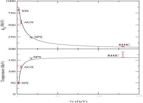
Figure 31: Behavior of the freeze–out baryon chemical potential $\mu_{B}$ (upper curve) and the temperature $T$ (lower curve) as a function of energy from Ref. (r42). The temperature $T$ as a function of beam energy is determined from the unified freeze–out conditions of fixed energy/particle.

We turn our attention first to a study of the energy dependence of the Wròblewski ratio defined as

$$\lambda_{s}\equiv{2\bigl{<}s\bar{s}\bigr{>}\over\bigl{<}u\bar{u}\bigr{>}+\bigl{<}d\bar{d}\bigr{>}},$$ (119)

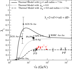
Figure 32: The Wròblewski ratio $\lambda_{s}$ as a function of $\sqrt{s}$. For the description of the lines see text. The points are the statistical model results calculated with thermal parameters obtained from the fit to measured particle yields.

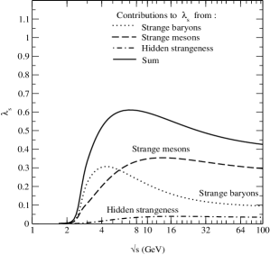
Figure 33: Contributions to the Wròblewski factor from strange baryons, strange mesons and hidden strange particles. Full line is a sum of all these contributions.

where the quantities in angular brackets refer to the number of newly formed quark-antiquark pairs, i.e., it excludes all the quarks that are present in the target and projectile.

The quark content used in this ratio is determined at the moment of chemical freeze–out, i.e. from hadrons and especially, hadronic resonances, before they decay. This ratio is thus not easily measurable unless one can reconstruct all resonances from the final-state particles.

The results are shown in Fig. (33) as a function of center of mass energy $\sqrt{s}$. The values calculated from the experimental data at chemical freeze–out in central A–A collisions have been taken from reference (r14). All values of $\lambda_{s}$ were extracted from fully integrated data besides RHIC where the STAR collaboration results

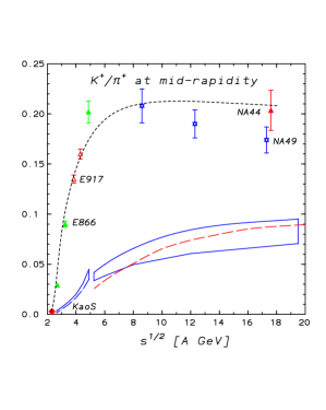
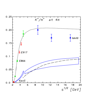
Figure 34: The ratio of kaon to pion measured in heavy ion collision at different collisions energies. The left-hand figure describes midrapidity data, whereas the right hand figure represents the ratio of fully integrated yields. Data at SIS, AGS, SPS and RHIC energy are taken from Refs. (na49aa,r85,r49). The short-dashed line describes the statistical model predictions along the unified freeze–out curve. The right hand figure also shows the parameterization of the p–p data (full-lines) from Ref. (ogilvie) and the canonical model results (dashed-line).

on particle ratios measured[190] at mid-pseudorapidity were used. The solid line in Fig. (33) describes the statistical model calculations[34] in complete equilibrium along the unified freeze–out curve and with the energy dependent thermal parameters shown in Fig. (31). From Fig. (33) one sees that around 30 $A\cdot$GeV lab energy the relative strangeness content in heavy ion collisions reaches a clear and well pronounced maximum. The Wròblewski factor decreases towards higher incident energies and reaches a limiting value of about 0.43.

The appearance of the maximum can be related to the specific dependence of $\mu_{B}$ on the beam energy. In Fig. (33) we also show $\lambda_{s}$ calculated under the assumption that only the temperature varies with collision energy but the baryon chemical potential is kept fixed at zero (dotted line). In this case the Wròblewski factor is indeed seen to be a smooth function of energy. The assumption of vanishing net baryon density is close to the prevailing situation in e.g. p–$\bar{\rm{p}}$ and e⁺–e^- collisions. In Fig. (33) the results for $\lambda_{s}$ extracted from the data in p–p, $\bar{\rm p}$–p and e⁺—e^- are also included[133]. The dashed line represents the results obtained with $\mu_{B}=0$ and a canonical radius of 1.2 fm. There are two important differences in the behavior of $\lambda_{s}$ in elementary compared to heavy ion collisions. Firstly, the strangeness content is smaller by a factor of two. This is mainly because in the elementary collisions particle multiplicities follow the values given by the canonical ensemble with radius 1.1-1.2 fm whereas in A-A collisions the grand canonical ensemble can be used, thus strangeness is uncorrelated and distributed in the whole fireball. Secondly, there is no evidence, at the moment, of a significant maximum in the behavior of $\lambda_{s}$ in elementary collisions.

The importance of finite net baryon density on the behavior of $\lambda_{s}$ is demonstrated in Fig. (33) showing separately the contributions to $\left<s\bar{s}\right>$ coming from strange baryons, strange mesons and from hidden strangeness, i.e., from hadrons like $\phi$ and $\eta$. As can be seen in Fig. (33), the origin of the maximum in the Wròblewski ratio can be traced to the contribution of strange baryons that is strongly enhanced in the energy range up to 30 A$\cdot$GeV.

The appearance of the maximum in the strangeness content of the collisions fireball can be also justified on the level of different ratios that includes strange particles. The measured[187, 190] $K^{+}/\pi^{+}$ ratio (see also Fig. (34)) is a very abruptly increasing function of the collision energy between SIS up to the top AGS energy. At higher energies it reaches a broad maximum between 20 A$\cdot$GeV - 40 A$\cdot$GeV and gradually decreases up to RHIC energy. In microscopic transport models[192] the increase of the kaon yield with collision energy is qualitatively expected as being due to a change in the production mechanism from associated to direct kaon emission. However, hadronic cascade transport models do not, until now, provide quantitative explanation of the experimental data in the whole energy range. This is evident in Fig. (35) where the comparisons of RQMD, URQMD and BUU microscopic transport

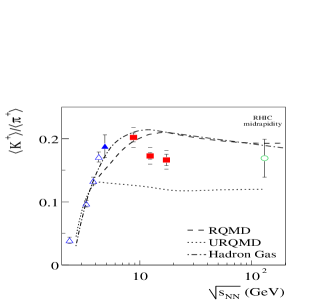
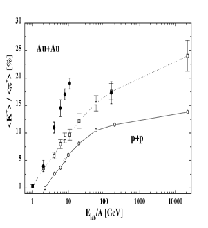
Figure 35: The ratio of kaon to pion measured in heavy ion collision at different collisions energies in comparison with microscopic transport models. The left-hand figure represents the RQMD[193], UrQMD[194, 125] and the statistical model predictions. The right hand figure shows the BUU results[192]. For the description of data see Refs. (r59,r48).

models with experimental data is presented. The RQMD provides a good description of the high energy data. The URQMD works quite well at the low energy, however, underestimates the yields at the SPS and RHIC energy. The BUU on the other hand is well suitable for SIS energy range, however, shows different energy dependence than that obtained in experiments. The statistical model in the canonical formulation[57],on the other hand, provides a good description of the $K/\pi$ midrapidity ratio from SIS up to AGS as seen in Fig. (34). The abrupt increase from SIS to AGS and the broad maximum of this ratio are consequences of the specific dependence of thermal parameters on the collision energy and the canonical strangeness suppression at SIS. A drop in the $K^{+}/\pi^{+}$ ratio for 4$\pi$ yields reported[187, 190] by the NA49 Collaboration at 158 A$\cdot$GeV (see Fig. (35) is, however, not reproduced by the statistical model without further modifications, e.g. by introducing an additional parameter $\gamma_{s}\sim 0.75$[40] that accounts for additional suppression of strangeness. We also note that an abrupt drop in the $K^{+}/\pi^{+}$ ratio is predicted[195] in a special model with particular conditions on the early stage of the collisions. This model, however, neglects completely the production of strange particles from the hadronization of gluons.

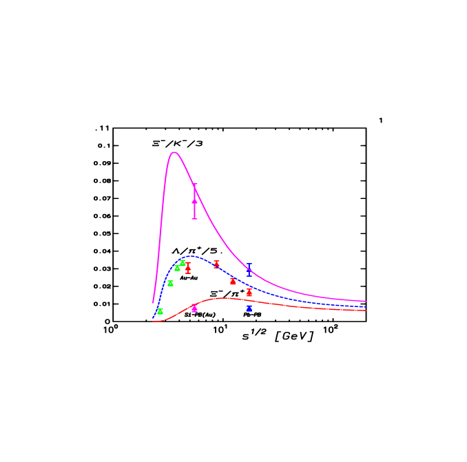
Figure 36: Particle ratios in A–A collisions versus the center-of-mass energy. Data at the SPS are fully integrated NA49 results. The corresponding ratio at the top AGS was obtained from E810 results on $\Xi^{-}$ measured[196] in Si–Pb collisions in the rapidity interval $1.4<y<2.9$, normalized to the full phase–space values of $\pi^{+}$ and $K^{-}$ yield obtained[197]in Si–Au collisions by E802 Collaboration. The lines represent statistical model results[53] along the unified freeze–out curve.

The appearance of the maximum in the relative strange/non-strange particle multiplicity ratios already seen in $K^{+}/\pi^{+}$ is even more pronounced[53] for strange baryon/meson ratios. Fig. (36) shows the energy dependence of $\Lambda/\pi^{+}$ and $\Xi^{-}/\pi^{+}$. There is a very clearly pronounced maximum, especially in the $\Lambda/\pi^{+}$ ratio. This maximum is related with a rather strong decrease of the chemical potential coupled with only a moderate increase in the associated temperature as the energy increases[53]. The relative enhancement of $\Lambda$ is stronger than that of $\Xi^{-}$. There is also a shift of the maximum to higher energies for particles with increasing number of strange quarks. This is because an enhanced strangeness content of the baryon suppresses the dependence of the corresponding ratio on $\mu_{B}$. This is also seen for $\Xi^{-}/K^{-}$ ratio that shows a substantially narrower maximum since the strangeness dilution effect is compensated by the strangeness content of the $K^{-}$. The actual experimental data for both $\Lambda/\pi^{+}$ and $\Xi^{-}/\pi^{+}$ ratios shown in Fig. (36) are following the predictions of the statistical model. However, as in the case of kaons, midrapidity results are better reproduced by the model than $4\pi$ data.

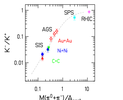
Figure 37: The left-hand figure, shows the ratio of $K^{+}/K^{-}$ as a function of $(\pi^{+}-\pi^{0})/A_{part}$. Points are the experimental results, a line is the statistical model result along the unified freeze-out curve. The right-hand figure shows $K^{-}/K^{+}$ ratio that appears to be constant as a function of centrality from SIS up to RHIC energy. Data are from the STAR, NA49, E866, and KaoS Collaborations. The broken lines are statistical model results.

The statistical model predicts that if at least two different ratios of non strange particles are constant with centrality then also strange particle/antiparticle ratio should be centrality independent. Dynamically this is a rather surprising result as strange particles and their antiparticles are generally produced and absorbed in the surrounding nuclear medium in a different way. This is particularly the case at lower energies (up to AGS) where e.g. $K^{+}$ and $K^{-}$ are predominantly produced due to $\pi N\to\Lambda K^{+}$ and $\pi\Lambda\to K^{-}N$ processes. In addition $K^{+}$, mesons feel a repulsive potential whereas $K^{-}$ mesons are attracted. Thus, the prediction of the thermal model that the $K^{+}/K^{-}$ ratio is centrality independent was dynamically unexpected. Figure (37) represents the energy and centrality dependence of the $K^{+}/K^{-}$ ratio from SIS to RHIC energy. The statistical model predictions are seen in Fig. (37 -right) to agree remarkably well with the data. The results of Fig. (37 -right) could be considered as the evidence of an apparent chemical equilibrium population of kaons in the final state. This behavior of data is also seen on a different level. The chemical equilibration of the associated production of $K^{+}$ with a hyperon and strangeness exchange production of $K^{-}$, indicated above, should result in a linear dependence of the $K^{+}/K^{-}$ ratio on $\pi/A_{part}$[198]. Fig. (37 - left) shows that, indeed, in the energy range from SIS up to AGS, and almost independently from the colliding system, the above prediction is valid. It is also clear from this figure that between AGS and SPS the production mechanism of strange mesons is changing.

The results for the $K^{+}$ and $K^{-}$ excitation function show an interesting behavior when expressed as a function of available energy $\sqrt{s}-\sqrt{s_{th}}$ (see Fig. (38 -left)[49]. The threshold energy $\sqrt{s_{th}}$ corresponds to the production threshold in N–N collisions. For $K^{+}$ mesons $\sqrt{s_{th}}$ = 2.548 GeV, whereas for $K^{-}$ the corresponding value is $\sqrt{s_{th}}$ = 2.87 GeV. It turned out that in this representation the measured yields of $K^{+}$ and $K^{-}$, close to threshold, in heavy ion collisions are about equal while they differ in p–p collisions by a factor of 10 – 100[199]. Fig. (38 -left) shows the experimental data together with the canonical statistical model results[49]. In the range where $\sqrt{s}-\sqrt{s_{th}}$ is less than zero, the excitation functions for $K^{+}$ and $K^{-}$, obtained in the model, cross each other, leading to the observed equality of $K^{+}$ and $K^{-}$ at SIS energies. The yields differ at AGS energies by a factor of five. The difference in the rise of the two excitation functions can be understood in the statistical model as being due to the different dependence of $K^{+}$ and $K^{-}$ yields on $\mu_{B}$. The $K^{+}$ yield is strongly $\mu_{B}$ dependent through associated production with $\Lambda$ whereas $K^{-}$ yield is not directly effected by $\mu_{B}$. Consequently, the excitation functions, i.e. the variation with $T$, exhibit a different rise for kaons and anti-kaons.

Figure 38: The left–hand figure: calculated $K^{+}/A_{part}$ and $K^{-}/A_{part}$ ratios of yield/participant in the statistical model as a function of $\sqrt{s}-\sqrt{s_{th}}$ for Ni+Ni collisions. The points are the results for Ni+Ni collisions at SIS[119, 120] and for Au+Au collisions at 10.2 $A\cdot$GeV (AGS)[121] energies. The right-hand figure: the yield of $\phi/K^{-}$ ratio in Ni–Ni and Au–Au collisions calculated[208] in the statistical model along the unified freeze–out curve. The data points are from Ref. (r99)

In the statistical model all particle species are considered to be on shell. Thus, the statistical model reproduces the kaon yields and their excitation functions with current particle masses. A transport calculation[130, 192, 128], on the other hand, required in–medium modifications (a reduction) of the $K^{-}$ mass (as expected for kaon in the nuclear medium) in order to describe the measured yields. These differences are, however not necessarily in contradiction, as the transport model describes a time evolution of particle production, whereas the statistical models are only valid for particles that are measured in the final state, where the on-shell conditions are to be expected. It is conceivable that the apparent chemical equilibration observed in the data at SIS energies could be a direct consequence of in–medium effects. One such possibility is an increase of the in–medium production cross section of strange particles.

In the context of particle production in heavy ion collisions a particular role has been attributed to the vector meson resonances. The measurements of these particles could possibly provide an information on the chiral symmetry restoration[4, 19, 24, 25, 27] and in medium effects due to the collision broadening[115] of their decay widths. The production of $\phi$ meson is of particular interest due to its $s\bar{s}$ content that could make it a very sensitive probe of strangeness production in the early stage. The yield of $\phi$ mesons at the SPS was found to be very different when it was reconstructed[201, 204] from the $K^{+}K^{-}$ or $\mu^{+}\mu^{-}$ decay channels. Possible scenarios of this difference were extensively discussed[205] in the literature. In view of the above problems it is interesting to check if the production of $\phi$ mesons follows the statistical order. Figure (38 -right) shows experimental values for the ratio of $\phi/K^{-}$ obtained at SIS[203, 206], AGS[200], SPS[201] and RHIC energies[202]. These results are compared[208] with the canonical model for Ni–Ni and Au–Au collisions. The $\phi/K^{-}$ ratio is seen in Fig. (38 -right) to exhibit a broad maximum as a function of collision energy that appears around 40 A$\cdot$GeV. Thus, the maximum strangeness content indicated in Fig. (36) is also visible here. It is surprising that the yield of $\phi/K^{-}$ within 40$\%$ is the same in a very broad energy range from AGS up to RHIC. The Ni–Ni results seems to follow this systematics. However, we have to point out that the most recent, still preliminary results[203] of the FOPI Collaboration indicate a much larger value of the ratio than it is shown in Fig. (38 -right). Also at the SPS the results[204] of the NA50 Collaboration, extrapolated with the measured slope to lower $p_{t}$, would give the value that is by a factor of $3-5$ larger then that obtained[201] by NA49 Collaboration. The above uncertainties notwithstanding, the statistical model follows the trend of data and reproduces their magnitude remarkably well. It is interesting to note the differences in the canonical model on the energy dependence of the $\phi/K^{-}$ for Ni–Ni and Au–Au collisions. The Ni–Ni line in Fig. (38 -right) shows a sharp minimum at $3<\sqrt{s}<4$ that appears due to a strong decrease of the $K^{-}$ yield through the canonical suppression. In the canonical model, applied here the $\phi$ meson yield is unconstraint. This would not be the case if the strangeness undersaturation factor, instead of the correlation volume, would be implemented.

Another interesting future of the $\phi$ yield is its centrality dependence. The ratio of $\phi/K^{-}$ measured at AGS[200], SPS[201] and RHIC[202] energies is centrality independent whereas both $\phi$ and $K^{-}$ are showing a strong centrality dependence that increases with decreasing beam energy. Thus, the $\phi$ meson shows a similar centrality dependence as kaons.

The centrality dependence of the $K/\pi$ ratio at the SPS was recently described[209, 210], in the context of a statistical model, as being due to centrality dependence of strangeness undersaturation parameter $\lambda_{s}$. This is quite a conceivable scenario. The $K^{+}/K^{-}$ as well as $\bar{p}/p$ ratios are only very weakly centrality dependent, thus the temperature and baryon chemical potential, should be rather constant with $A_{part}$. The change of the $K/\pi\sim\lambda_{s}$ with $A_{part}$ could be thus attributed to $\lambda_{s}$. The same arguments could be also applied to the AGS and RHIC results. However, the $\phi/K^{-}$ is to be proportional to $\lambda_{s}$, consequently the $\phi/K^{-}$ ratio should show similar $A_{part}$ dependence as $K/\pi$ ratio. The above, however, is not confirmed experimentally. This discrepancy calls into question the concept of a $\gamma_{s}$ factor as the relevant parameter characterizing strangeness production in heavy ion collisions (see also the discussion in Section 2).

7 Lifting of the strangeness suppression in heavy ion collisions

An enhanced production of strange particles compared to the suppressed strangeness yield observed in collisions between elementary particles was long suggested[31, 42, 43] as a possible signal of the QGP formation in heavy ion collisions. In the QGP the production and equilibration of strangeness is very efficient due to a large gluon density and a low energy threshold for dominant QCD processes of $s\bar{s}$ production[31, 32]. In hadronic systems the higher threshold for strangeness production was argued in Ref. (r34) to make the strangeness yield considerably smaller and the equilibration time much longer.

Based on such arguments predictions have been developed for experimental signatures of deconfinement. Key predictions are[31, 52]:

i) the disappearance of the strangeness suppression observed in collisions among elementary particles leading to e.g. an enhancement of multistrange baryons and anti-baryons in central A–A collisions, with respect to proton induced reactions.

ii) chemical equilibration of secondaries: the appearance of the QGP being close to a chemical equilibrium and subsequent phase transition should in general drive hadronic constituents produced from hadronizing QGP towards chemical equilibrium.

Heavy ion experiments at the CERN SPS reported[212, 213] actually a global increase of strangeness production from p-p, p-A to A-A collisions. This effect is seen e.g. in Fig. (34 -right) that shows the enhancement of the $K^{+}/\pi^{+}$ ratio in Pb–Pb relative to p+p collisions. There is indeed an increase by a factor of about two in strangeness content when going from p+p to heavy ion collisions. This is also seen on the level of the Wròblewski factor in Fig. (33).

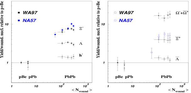
Figure 39: Particle yields per participant in Pb–Pb relative to p–Be and p–Pb collisions centrality dependence. The data are from WA97[212] and NA57[213] Collaborations.

A large strangeness content of the QGP plasma should, following (ii), be reflected in a very specific hierarchy of multistrange baryons[31]: implying an enhancement of $\Omega>\Xi>\Lambda$. Fig. (39) shows the yield/participant in Pb–Pb relative to p–Be and p–Pb collisions measured[212, 213] by the WA97 and NA57 Collaborations. Indeed the enhancement pattern of the antihyperon yields is seen to increase with strangeness content of the particle and in WA97 data there is a saturation of this enhancement for $N_{wound}>100$. The recent results of the NA57 collaboration are showing in addition an abrupt change of the anti-cascade enhancement for a lower centrality. Similar behavior was previously seen on the level of $K^{+}$ yield measured[214] at $\theta_{lab}=0$ by the NA52 experiment in Pb-Pb collisions. These results are very interesting as they might be interpreted as an indication of the onset of a new dynamics. However, a more detailed experimental study and theoretical understanding are still required here. Until now there is no quantitative understanding of this exceptional threshold behavior of $\bar{\Xi}$.

A number of different mechanisms were considered to describe the magnitude of the enhancement and centrality dependence of (multi)strange baryons measured[48, 189, 209, 215]^-[220] by the WA97 Collaboration. Studies using microscopic transport models make it clear that data shown in Fig. (39) can not be explained by pure final state hadronic interactions. The combination of the former with additional pre-hadronic mechanisms like sting formation and their subsequent hadronization, baryon junction mechanism, color ropes or a color flux tubes overlap improves the agreement with the measured enhancement pattern and the magnitude for the most central collisions. However, the detailed centrality dependence is still not well reproduced within the microscopic models.

The results of Section 2 have shown that the statistical model provides a satisfactory description of strange and multistrange particle yields in A–A collisions. The midrapidity data were argued in Section. 1 to be reproduced by the statistical model in a full equilibrium. The fully integrated results, on the other hand can be successfully reproduced when including a strangeness undersaturation parameter $\gamma_{s}\simeq 0.75$ that accounts, at the SPS, for a 25$\%$ deviation from equilibrium.

Strangeness production in p–p collisions was shown in Section 5 to be consistent with the canonical statistical model. The abundance of single-strange particles could be described by this model by including, as in heavy ion collisions, the strangeness undersaturation factor $\gamma_{s}\simeq 0.51$ or a correlation volume $V\sim V_{p}$ that accounts for the locality of strangeness conservation. Consequently, the enhancement from p–p to A–A collisions of strangeness 1 particles could be well described in terms of the statistical model as the transition from the canonical to the asymptotic GC limit[48].

Figure 40: The left hand figure: the canonical suppression factor $F_{s}\sim I_{s}(Vx)/I_{0}(Vx)$ as a function of $V\sim\langle N_{part}\rangle$ with the argument $x$ calculated for a hadron resonance gas at $T=168$ MeV and $\mu_{B}=266$ MeV. The right hand figure: statistical model results on centrality dependence of the relative enhancement of $4\pi$ particle yields/participant in central Pb–Pb to p–p collisions expected at $\sqrt{s}\simeq 17$ GeV.

One of the consequences of the canonical model is a very particular volume dependence of multistrange particle densities. In heavy ion collisions this volumes is usually assumed to scale with the number of participants. From Eq. (97) it is clear that the canonical suppression should increase with strangeness content of the particles. Indeed the approximate strangeness suppression factor $F_{s}\sim I_{s}(Vx)/I_{0}(Vx)$ for a fixed $Vx$ is a decreasing function of $s$. This is particularly evident in the limit of $(Vx)<<1$ where $I_{s}(Vx)/I_{0}(Vx)\sim(Vx)^{s}$. The suppression factor is quantified in Fig. (40 -left) that indicates the expected suppression pattern.

Fig. (41 -left) shows predictions[48] of the canonical model for the multiplicity/participant of $\Omega,~{}\Xi,$ and $\Lambda$ relative to their value in p–p collisions. Thermal parameters, $T=168$ MeV and $\mu_{B}=266$ MeV, that are appropriate[38] for a description of central Pb–Pb collisions at 160 A$\cdot$GeV, were used here and assumed to be centrality–independent. The canonical volume parameter was taken to be proportional to the number of projectile participants, $V\simeq V_{0}N_{\rm part}/2$ where $V_{0}=4\pi R_{p}^{3}/3$ with $R_{p}=1.15\pm 0.5$. The volume $V_{0}$ is then, depending on the particular choice of $R_{p}$, of the order of the volume of a nucleon. Figure (40 -right) indicates that the statistical model in the canonical ensemble reproduces the basic features of WA97 data: the enhancement pattern and enhancement saturation for large $A_{\rm part}$. The appearance of the saturation of the enhancement indicates that the grand canonical limit was reached. It is also clear from Fig. (41-left) that this saturation is shifted towards a larger centrality with increasing strangeness content of the particle.

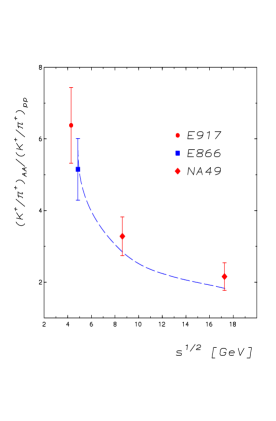
Figure 41: The left hand figure: the statistical model results on the centrality dependence of the relative enhancement of $\Lambda$, $\Xi$ and $\Omega$ yields/participant in central Pb–Pb to p–p collisions at $\sqrt{s}=8.73$ GeV. The right hand figure: $K^{+}/\pi^{+}$ ratio in A+A relative to p+p collisions. For the compilation of data, see Refs. (ogilvie,r49). The dashed line represents the statistical model results.

The essential prediction[44] of the canonical statistical model is that the strangeness enhancement from p–p to A–A collisions should increase with decreasing collision energy. This is a direct consequence of e.g. Eq. (97) where the canonical suppression factor is seen to be a decreasing function of temperature and thus also collision energy. Fig. (41 -right) shows the compilation of data on the $K^{+}/\pi^{+}$ ratio in A–A relative to p–p collisions from Ref. (ogilvie,r49). This double ratio could be referred to as a strangeness enhancement factor. The enhancement is seen in data to be the largest at the smallest beam energy and is decreasing towards higher energy. The line is a smooth interpolation between the canonical model results for $\sqrt{s}=17.3,12.3,8.73,5.56$ GeV, calculated with the thermal parameters $T$ and $\mu_{B}$ that were extracted from Fig. (27). The canonical volume parameter was taken the same as used in Fig. (16- right). The enhancement seen in Fig. ( 41 -right) is due to the suppression of the $K^{+}/\pi^{+}$ ratio in p–p collisions with decreasing energy and not due to a dilution of this ratio by excess pions in the A–A system. The $K^{+}/\pi^{+}$ ratio is known experimentally not to vary within $30\%$ in the energy range from $\sqrt{s}\sim 5$ GeV at AGS up to $\sqrt{s}=130$ GeV at RHIC[187, 190, 191]. Recent data of NA49[187] and CERES[168, 189] Collaborations on $\Lambda$ yields exhibit a similar energy dependence of the enhancement factor as is seen in Fig. (41- right) for kaons.

The canonical model (see Eq. (97)) also predicts that the multistrange baryon enhancement from p–p to A–A should be larger at lower collision energy. Fig. (41- left) shows the canonical model results for the strangeness enhancement and its centrality dependence for Au–Au collisions at 40 A$\cdot$GeV. The qualitative behavior of the enhancement is like that at the SPS. However, the strength of the enhancement is seen to be substantially larger. For $\Omega$ it can be as large as a factor of 100. The enhancement of $\Xi$ in A–A relative to p–p can be deduced from data. Indeed, combining the Si–Pb results for $\Xi^{-}$ production obtained[196] by E810 Collaboration and the Si–Au results for pion or $K^{-}$ yields obtained[197] by E802 Collaboration in collisions at the top AGS energy, one can estimate that $\Xi^{-}/\pi^{+}\sim 0.0076$. Within errors this agrees with the value of $\Xi^{-}/\pi^{+}\sim 0.0074$ obtained[138] by NA49 in Pb–Pb at $\sqrt{s}=17.3$ GeV, as seen in Fig. (36). In p–p collisions the $\Xi^{-}/\pi^{+}$ ratio is obviously a strongly decreasing function of beam energy. From the above one would therefore expect that the relative enhancement of $\Xi^{-}$ from p–p to A–A collisions should be larger at AGS than at SPS energy. This is seen in Fig. (41 -left). In addition ratios containing only newly produced particles, such as e.g. $\Xi^{-}/K^{-}$, are also larger at AGS than at SPS energy, see Fig. (36). The above heuristic argument should be, however, verified by more complete experimental data.

Recently, the production of $\Xi^{-}$ was study[218] in the relativistic transport model in the energy range from 2-11 A$\cdot$GeV . The authors discussed the equilibration and the influence of a phase transition on $\Xi$ yields in A–A collisions. There, it was argued that, for beam energies above 4 A$\cdot$GeV, there should be a sharp increase of the $\Xi^{-}$ yield if there is a deconfinement transition in the collisions fireball. This is an interesting conjecture. However, with the presently available experimental data this prediction cannot be tested. The canonical statistical model, predicts continuous increase of $\Xi$ yield with collisions energy as it is seen in Fig. (36).

The prediction of the statistical model on the energy dependence of strange particle yields is also in contrast with the UrQMD results[219]. There, the production of strangeness is very sensitive to the initial conditions. In UrQMD the early stage multiple scattering may imply an increase of the colour electric field strength due to an overlap of produced strings[219]. Consequently, according to the Schwinger mechanism, this should increase the production of (multi)strange baryons. Under similar kinematical conditions as at the SPS, the UrQMD model predicts[219] at RHIC an increase in relative strength of $\Omega$ yields from p–p to A–A by a factor of 5. A recent analysis of multistrange baryon yields in Au–Au collisions at RHIC energy in the context of Dual Parton Model, leads[139] to a smaller increase of the enhancement at RHIC energies.

The interpretation that the strangeness enhancement is explained by canonical effects is not necessarily in contradiction with the heuristic predictions[31] that strangeness enhancement and its pattern are due to a quark–gluon plasma formation in A–A collisions. This is particularly the case if one connects the asymptotic grand canonical description of strangeness production in A–A collisions with the formation of a QGP in the initial state.

8 Conclusions and outlook

This article has focussed almost exclusively on the use of the statistical approach to understand yields of different particle species that have been measured in heavy ion collisions. We have discussed a statistical description of the conservation laws and described their kinetic implementations. We have argued, both on the qualitative and quantitative level, that exact conservation of quantum numbers is of crucial importance when applying the methods of statistical physics in the context of heavy ion and particle collisions. We have presented the systematics of particle production in heavy ion collisions from SIS up to LHC energy and discussed particular properties of strangeness production. One of the most intriguing results that comes from these investigations is the observation that particles seem to be produced according to the principle of the maximal entropy. In a very broad energy range, from $\sqrt{s}\sim 2.5$ up to 200 GeV per nucleon pair, hadronic yields and their ratios observed in heavy ion collisions resemble a chemical equilibrium population along a unified freeze–out curve determined by the conditions of fixed energy/hadron $\simeq 1$GeV or complementary above SIS energy by fixed total density of baryons. Strangeness production follows this systematics from low to very high energy. However, there are some characteristic features of the system at chemical freeze–out in high energy central A+A collisions regarding strangeness production that are not present in low energy heavy ion and collisions among elementary particles. In nucleus–nucleus collisions, strangeness is un-correlated and redistributed in the macroscopic volume of a collision fireball and is conserved on the average. In hadron–hadron collisions the thermal phase space available for strange particles is strongly suppressed since, with only few particles produced per event, strangeness is strongly correlated in a volume that approximately coincides with the size of a nucleon, i.e. a distance over which color is confined. Thus, following the statistical kinetics, strangeness has to be conserved exactly and locally. The associated production and locality of strangeness conservation is, in the context of the statistical model, the origin of the suppression of the thermal phase space for produced particles. Within this context the strangeness suppression observed in collisions among elementary particles finds its natural explanation. We also note that the suppression increases with the strangeness content of the particle as well as, for A–A collisions, with decreasing collision energy. A further consequence of the transition from the canonical to the grand-canonical regime is that strangeness production should be enhanced in A–A collisions compared to p–p collisions.

At SPS and RHIC energies the freeze–out points approach the calculated QCD phase boundary. This fact lends strong support to the interpretation that the matter produced in nuclear collisions at SPS and RHIC energies was first thermalized in the deconfined quark-gluon plasma phase and subsequently expanded through the phase boundary into a thermal gas of mostly elastic and quasi–elastic interacting hadrons. The above connection between the QCD phase boundary and the observed chemical freeze–out points is sometimes called into question[221] since hadron production in $e^{+}e^{-}$ and p–p or p–$\bar{\rm{p}}$ can also be described in thermal models yielding a (apparently universal) temperature T${}_{e}\approx 170$ MeV. While the fact that T_e is close to T values determined for heavy ion collisions at top SPS and RHIC energies might indeed reflect the fundamental hadronization scale of QCD, we have already noted above that there is an essential difference between thermal descriptions of central heavy ion collisions and elementary particle reactions. Strange particle densities and their ratios can be, for heavy ion collisions at full AGS energy and higher, well described in the grand-canonical ensemble. In contrast, for a description of particle production in elementary collisions, local quantum number conservation, that is the canonical description is need. Consequently, in central nucleus-nucleus collisions at ultra-relativistic energies, strangeness percolates freely over volumes of thousands of fm³! whereas in elementary processes is approximately restricted to the size of nucleon. At top SPS and RHIC energies it is natural to conclude that in nucleus–nucleus collisions the percolation has its origin in the quark-gluon phase, lending further strong support to the interpretation that the ``coincidence'' between experimentally determined chemical freeze–out points and the calculated phase boundary implies that a deconfined phase was produced in such collisions.

In the context of statistical physics the fact that the measured particle yields coincides with a thermal multiplicities calculated with a given statistical operator is a necessary and sufficient conditions to maintained thermalization of the collisions fireball. In the sense of Gibbs interpretation of thermodynamics this implies that the parameters $T$ and $\mu_{B}$ reflect the thermal properties of the fireball. Furthermore in heavy ion collisions there are experimental observables indicating the appearance of thermodynamical pressure and correlations that are expected in a thermalized medium. The build–up of pressure and collectivity is seen in heavy ion collisions on the level of particle transverse momentum distributions and elliptic flow parameters. An increase of average particle transverse momentum with particle mass, seen from SIS up to RHIC energy, is a typical property of a transversally expanding thermal medium. The appearance of strong elliptic flow is an indication of thermodynamical pressure that develops in the early stage in the collision. Finally, the measured particle number fluctuations are consistent with thermal expectations. Taken together, these observations lend strong support to the thermodynamic interpretation of $T$ and $\mu_{B}$ with the concomitant QGP interpretation.

References

- [1] For a review see eg. H. Satz, Rep. Prog. Phys. 63 (2000) 1511; S.A. Bass, M. Gyulassy, H. Stöcker, and W. Greiner, J. Phys. G25 R1 (1999). E.V. Shuryak, Phys. Rep. 115 (1984) 151; M.G. Alford, hep-ph/0209287, H. Satz, hep-ph/0209181.
- [2] J. Cleymans, R.V. Gavai and E. Suhonen, Phys. Rep. 130 (1986) 217.
- [3] B. Alessandro, et al., CERN-ALICE-INTERNAL-NOTE-2002-025.
- [4] G.E. Brown and M. Rho, Phys. Rep. 363 (2002) 85.
- [5] W. Cassing and H. Bratkovskaya, Phys. Rep. 308 (1999) 65.
- [6] P. Braun-Munzinger, and J. Stachel, Nucl. Phys. A606 (1996) 320; Nucl. Phys. A683 (1998) 3; J. Stachel, Nucl. Phys. A654 (1999) 119c.
- [7] R. Stock, Phys. Lett. B456 (1999) 277.
- [8] R. Baier, A.H. Mueller, D. Schiff, and D.T. Son, Phys. Lett. B 502 (2001) 51; Nucl. Phys. A698 (2002) 217.
- [9] U. Heinz, Nucl. Phys. A685 (2001) 414 and A661 (1999) 349.
- [10] K. J. Eskola, K. Kajantie, P. Ruuskanen and K. Tuominen, Nucl. Phys. B570 (2000) 379.
- [11] J. Alam, et al., hep-th/010802; Ann. Phys. 286 (2001) 159.
- [12] D. K. Srivastava, Eur. Phys. J. 10 (1999) 487.
- [13] R. Rapp, Phys. Rev. C63 (2001) 054907.
- [14] V. Ruuskanen, Acta. Phys. Polon. B18 (1987) 551; R. Rapp, and E. Shuryak, Phys. Lett. B473200013; I. Krasnikova, Ch. Gale, and D.K. Srivastava, Phys. Rev. C65 (2002) 064903, hep-ph/0112139; Ch. Gale, Nucl.Phys. A698 (2002) 143c, hep-ph/0104235.
- [15] R. Rapp and J. Wambach, Phys. Rev. C55 (1998) 916; Nucl. Phys. A638 (1998) 171c; Eur. Phys. J. A6 (1999) 415.
- [16] K. Gallmeister, B. Kämpfer, and O.P. Pavlenko, Phys. Lett. B473 (2000) 20.
- [17] F. Karsch, K. Redlich, and L. Turko, Z. Phys. C60 (1993) 519.
- [18] K. Kajanie, J. Kapusta, L.D. McLerran, and A. Mekjian, Phys. Rev. D34 (1986) 2746 .
- [19] T. Hatsuda, Nucl. Phys. A698 (2002) 243; K. Yokokawa, et al., Phys. Rev. C66 (2002) 022201; D. Jido, et al., Phys. Rev. D63 (2001) 011901.
- [20] D. Teaney, J. Lauret, and E. Shuryak, Phys. Rev. Lett. 86 (2001) 4783.
- [21] U.A. Wiedemann and U. Heinz, Phys. Rep. 319 (1999) 145, and references therein.
- [22] B. Tomasik, U.A. Wiedemann and U. Heinz, Nucl. Phys. A663 (2000) 753; R. Nix, Phys. Rev. C58 (1998) 2303.
- [23] Nu Xu, nucl-ex/0211012.
- [24] V. Metag, Nucl. Phys. A690 (2001) 140.
- [25] W. Weinhold, B.L. Friman and W. Nörenberg, Acta. Phys. Polon. B27 (1996) 3249; Phys. Lett. B433 (1998) 236; M. Hermann, B.L. Friman and W. Weinhold, Nucl. Phys. A545 (1992) 2676.
- [26] G. Boyd, et al., Nucl. Phys. Proc. Suppl. 42 (1995) 469; Phys. Lett. B349 (1995) 170; E. Laermann, et al., Nucl. Phys. Proc. Suppl. 34 (1994) 292.
- [27] M.F.M. Lutz, G. Wolf and B. Friman, Nucl. Phys. A706 (2002) 431; Nucl. Phys. A661 (1999) 526.
- [28] T. Matsui and H. Satz, Phys. Lett. B178 (1986) 416.
- [29] H. W. Barz, H. Schulz, B.L. Friman and J. Knoll, Phys. Lett. B254 (1991) 315, Nucl. Phys. A545 (1992) 259.
- [30] T.S. Biro, hep-ph/0005067, hep-ph/0205049; T.S. Biro, Phys. Lett. B487 (2000) 133.
- [31] P. Koch, B. Müller, and J. Rafelski, Phys. Rep. 142 (1986) 167; J. Rafelski, J. Letessier, and A. Tounsi, Acta Phys. Polon. B27 (1996) 1037; J. Rafelski Phys. Lett. B262 (1991) 333.
- [32] T. Matsui, B. Svetitsky and L.D. McLerran, Phys. Rev. D34 (1986) 783.
- [33] R. Rapp and E. Shuryak, Phys. Rev. Lett. 86 (2001) 2980; C. Greiner and S. Leupold, J. Phys. G27 (2001) L95.
- [34] J. Cleymans, and K. Redlich, Phys. Rev. Lett. 81 (1998) 5284.
- [35] P. Braun-Munzinger, D. Magestro, K. Redlich, and J. Stachel, Phys. Lett. B518 (2001) 41 and references therein.
- [36] D. Magestro, J. Phys. G28 (2002) 1745.
- [37] P. Braun-Munzinger, J. Stachel, J.P. Wessels and N. Xu, Phys. Lett. B344 (1995) 43 and B365 (1996) 1.
- [38] P. Braun-Munzinger, I. Heppe and J. Stachel, Phys. Lett. B465 (1999) 15.
- [39] S.V. Akkelin, P. Braun-Munzinger and Yu. M. Sinyukov, Nucl. Phys. A710 (2002) 439.
- [40] F. Becattini, J. Cleymans, A. Keranen, E. Suhonen and K. Redlich, Phys. Rev. C64 (2001) 024901.
- [41] A. Keranen, and F. Becattini, J. Phys. G28 (2002) 2041; Phys. Rev. C65 (2002) 044091.
- [42] J. Rafelski and J. Letessier, nucl-th/0209080.
- [43] M. Gazdzicki, et al., Z. Phys. C65 (1995) 215, Acta Phys. Polon. B30 (1999) 2705.
- [44] A. Tounsi and K. Redlich, Eur. Phys. J. C24 (2002) 529; J. Phys. G28 (2002) 2095.
- [45] F. Becattini, hep-ph/0202071.
- [46] J. Sollfrank, et al., Phys. Rev. C55 (1997) 392.
- [47] P. Huovinen, et al., Phys. Lett. B503 (2001) 58.
- [48] J. S. Hamieh, K. Redlich and A. Tounsi, Phys. Lett. B486 (2000) 61; J. Phys. G27 (2001) 413.
- [49] J. Cleymans and K. Redlich, Phys. Rev. C60 (1999) 054908; J. Cleymans, H. Oeschler and K. Redlich, Phys. Rev. C59 (1999) 1663; Phys. Lett. B485 (2001) 27.
- [50] J. Cleymans, D. Elliott, A. Keranen and E. Suhonen, Phys. Rev. C57 (1998) 3319.
- [51] D. Zschiesche et al., Nucl. Phys. A681 (2001) 34.
- [52] J. Letessier, and J. Rafelski, Int. J. Mod. Phys. E9 (2000) 107.
- [53] P. Braun-Munzinger, J. Cleymans, H. Oeschler and K. Redlich, Nucl. Phys. A697 (2002) 902.
- [54] N. Xu, M. Kaneta, Nucl. Phys. A698 (2002)306, nucl-ex/0104021; M. Kaneta and N. Xu, J. Phys. G27 (2001) 589; Nucl. Phys. A698 (2002) 306.
- [55] W. Broniowski and W. Florkowski, Phys. Rev. Lett. 87 (2001) 272302.
- [56] F. Becattini and G. Passaleva, Eur. Phys. J. C23 (2002) 551, hep-ph/0110312.
- [57] K. Redlich, Nucl. Phys. A698 (2002) 94.
- [58] J. Cleymans and H. Satz, Z. Phys. C57 (1993) 135.
- [59] D. Magestro, P. Braun-Munzinger, and J. Stachel, in preparation.
- [60] I. Heppe, Diploma thesis, Heidelberg(1998).
- [61] G. Yen, M.I. Gorenstein, W. Greiner, S.N. Yang, Phys. Rev. C 56, (1997) 2210.
- [62] see, e.g., A. Bohr and B. Mottelson, Nucl. Structure (Benjamin, New York 1969), Vol. 1, p. 266.
- [63] D. Ouerdane et al., BRAHMS Coll., QM2002 contribution, Nucl. Phys. A (in print), nucl-ex/0212001.
- [64] T. Ullrich, QM2002 contribution, nucl-ex/0211004, Nucl. Phys. A (in print).
- [65] J. Cleymans in 3rd International Conference on Physics and Astrophysics of Quark Gluon Plasma (ICPAQGP 97), Jaipur, India, 17-21 Mar 1997.
- [66] H. Appelshäuser et al., NA49 Coll., Phys.Rev.Lett. 82 (1999) 2471.
- [67] T.S. Biro, P. Levai, J. Zimanyi, J.Phys. G28 (2002) 1561, hep-ph/0112137; J. Zimanyi, et al., in S.A. Bass, et al., Nucl. Phys. A661 (1999) 205c.
- [68] J. Rafelski, J. Letessier, Qm2002 contribution, nucl-th/0209084, Nucl. Phys. A(in print); J. Rafelski, et al., in S.A. Bass, et al., Nucl. Phys. A661 (1999) 205c.
- [69] P. Fachini et al., STAR Coll., QM2002 contribution, nucl-ex/0211001, Nucl. Phys. A (in print).
- [70] D. Adamova et al., CERES coll., Nucl.Phys. A714 (2003) 124, nucl-ex/0207005.
- [71] D. Adamova et al., CERES coll., Phys.Rev.Lett. 90 (2003) 022301, nucl-ex/0207008.
- [72] M. van Leeuwen et al., NA49 coll., QM2002 contribution, Nucl. Phys. A (in print), nucl-ex/0208014.
- [73] J. Barrette et al., E814 Coll., Phys. Lett. B333 (1994) 33.
- [74] N. Xu et al., E814 Coll., Nucl. Phys. A566 (1994) 585c.
- [75] P. Braun-Munzinger and J. Stachel, Phys. Lett. B490 (2000)196 ; Nucl. Phys. A690 (2001) 119c.
- [76] P. Braun-Munzinger and J. Stachel, Nucl. Phys. A690 (2001) 119c.
- [77] F. Karsch, E. Laermann, and A. Peikert, Nucl. Phys. B605 (2001)579.
- [78] J.D. Bjorken, Phys. Rev. D27 (1983) 140.
- [79] F. Karsch, K. Redlich, and A. Tawfik, hep-ph/0303108.
- [80] P. Braun-Munzinger, J. Stachel, and C. Wetterich, in preparation.
- [81] J.P. Blaizot, E. Iancu, and A. Rebhan, Phys. Rev. D63 (2001) 065003.
- [82] E. Suhonen and S. Sohlo, J. Phys. G13 (1987) 1487; D. H. Rischke, M. I. Gorenstein, H. Stöcker and W. Greiner, Z. Phys. C51 (1991) 485.
- [83] A. Peshier, B. Kämpfer, and G. Soff, Phys. Rev. C61 (2000) 045203; Phys. Rev. D66 (2002) 094003; B. Kämpfer, and O.P. Pavlenko, Phys. Lett. B391 (1997) 185.
- [84] R. Pisarski, Phys. Rev. D62 (2000) 111501.
- [85] A. Dumitru and R.D. Pisarski, Phys. Lett. B525 (2002) 95; A. Dumitru and R.D. Pisarski, Phys. Rev. D66 (2002) 096003, hep-ph/0204223.
- [86] M. Agarwal, et al., WA98 Coll., Eur. Phys. J. C18 (2001) 651.
- [87] L. V. Gribov, et al., Phys. Rep. 100 (1983) 1; A.H. Mueller and J. Qiu, Nucl. Phys. B268 (1986) 427.
- [88] L.D. McLerran, and R. Venugopalan, Phys. Rev. D49 (1994) 2233; Phys. Rev. D49 (1994) 3352; Phys. Rev. D50 (1994) 2225.
- [89] D. Kharzeev and M. Nardi, Phys. Lett. B507 (2001) 121.
- [90] E.V. Shuryak, and L. Xiong, Phys. Rev. Lett. 70 (1993) 2241; J. Kapusta, L. McLerran, and D.K. Srivastava, Phys. Lett. B283 (1992) 145.
- [91] Particle Properties
- [92] D. K. Srivastava, M. G. Mustafa, and B. Müller, Phys. Rev. C56 (1977) 1064; R.J. Fries, B. Müller and D. K. Srivastava, nucl-th/0208001.
- [93] K. Geiger and D. K. Srivastava, Nucl. Phys A661 (1999) 592, nucl-th/9808042.
- [94] K. Huang, Statistical Mechanics, 2nd Edition, Wiley, New York, 1987, sect. 3.4.
- [95] T. A. Armstrong, et al., E864 Coll., Phys. Rev. C61 (2000) 064908.
- [96] T. A. Armstrong, et al., E864 Coll., Phys. Rev. Lett. 85 (2000) 2685.
- [97] P. Braun-Munzinger, and J. Stachel, J. Phys. G: Nucl. Part. Phys. 21 (1995) L17.
- [98] A.J. Baltz et al., Phys. Let. B325 (1994) 7.
- [99] C.M. Ko, V. Koch, Z. Lin, K. Redlich, M. Stephanov and X.N. Wang, Phys. Rev. Lett. 86 (2001) 5438.
- [100] S. Jeon, V. Koch, K. Redlich and X.N. Wang, Nuc. Phys. A697 (2002) 546; K. Redlich, V. Koch and A. Tounsi, Nucl. Phys. A702 (2002) 326; K. Redlich, J. Cleymans, H. Oeschler, and A. Tounsi, Acta Phys. Polon. B33 (2002) 1609.
- [101] Z. Lin, and C.M. Ko, Phys. Rev. C64 (2001) 041901.
- [102] H.-Th. Elze, M. Gyulassy, and D. Vasak, Nucl. Phys. B276 (1986) 706.
- [103] J.P. Blaizot, and E. Iancu, Nucl. Phys. B 570 (2000) 326.
- [104] Q. Wang, K. Redlich, H. Stöcker, and W. Greiner, Phys. Rev. Lett. 88 (2002) 132303; Nucl. Phys. A714 (2003) 293; J. Phys. G28 (2002) 2115.
- [105] R. Hagedorn, Thermodynamics of strong interactions, CERN Report 71-12 (1971); E.V. Shuryak, Phys. Lett. B42 (1972) 357; Rafelski and M. Danos, Phys. Lett. B97 (1980) 279; R. Hagedorn and K. Redlich, Z. Phys. C27 (1985) 541.
- [106] R. Hagedorn and K. Redlich, Z. Phys. C27 (1985) 541.
- [107] K. Redlich and L. Turko, Z. Phys. B97 (1980) 279; L. Turko, Phys. Lett. B104 (1981) 153; L. Turko and J. Rafelski, Eur. Phys. J. C18 (2001) 587.
- [108] K. Redlich, F. Karsch, and A. Tounsi, hep-ph/0302245.
- [109] J. Cleymans and P. Koch, Z. Phys. C52 (1991) 137.
- [110] D. Miller and K. Redlich, Phys. Rev. D37 (1988) 3716; Phys. Rev. D35 (1987) 2524; H. Th. Elze, D. Miller and K. Redlich, Phys. Rev. D35 (1987) 748.
- [111] H. Th. Elze, W. Greiner and J. Rafleski, Phys. Lett. B124 (1983) 515; Z. Phys. C24 (1984) 361; Ch. Derreth, W. Greiner, H. Th. Elze and J. Rafelski, Phys. Rev. C31 (1985) 1360; H. Th. Elze and W. Greiner, Phys. Rev. A33 (1986) 1879.
- [112] D.H. Rischke, M.I. Gorenstein, A. Schafer, H. Stöcker and W. Greiner, Phys. Lett. B278 (1992) 19; D.H. Rischke, J. Schaffner, M.I. Gorenstein, A. Schaefer, H. Stöcker and W. Greiner, Z. Phys. C56 (1992) 325.
- [113] A. Gocksch, R.D. Pisarski, Nucl. Phys. B402 (1993) 657.
- [114] J. Engels, et al., Z. Phys. C42 (1989) 341; A. Peshier, et al., Phys. Rev. C61 (2000) 045203 and references therein.
- [115] R. Rapp and J. Wambach, Adv. Nucl. Phys. 25 (2000) 1.
- [116] J. Cleymans, K. Redlich and E. Suhonen, Z. Phys. C58 (1993) 347.
- [117] K. Zalewski, Acta. Phys. Polon. B62 (1965) 933.
- [118] A. Wagner et al., KaoS Coll., Phys. Lett. B420 (1998) 20, C. Müntz et al., KaoS Coll., Z. Phys. C357 39.
- [119] R. Barth et al., KaoS Coll., Phys. Rev. Lett. 78 (1997) 4007; F. Laue et al., KaoS Coll., Phys. Rev. Lett. 82 (1999) 1640.
- [120] M. Menzel, Ph.D.Thesis, Universität Marburg, 2000.
- [121] L. Ahle et al., E-802 Coll., Phys. Rev. C58 (1998) 3523;
- [122] R. Averbeck, R. Holzmann, V. Metag and R.S. Simon, nucl-ex/0012007; A.R. Wolf et al.,Phys. Rev. Lett. 80 (1998) 5281; By TAPS Coll., Z. Phys. A359 (1997) 65; Phys. Rev. C56 (1997) 2920.
- [123] B. Hong et al., FOPI Coll., Phys. Rev. C57 1998 244.
- [124] C. Müntz et al., KaoS Coll., Z. Phys. C357 1997 399; J. Phys. G28 (2002) 1895; Euro. Phys. J. A9 (2000) 397.
- [125] M. Bleicher et al., J. Phys. G25 (1999) 1859; S. A. Bass et al., Prog. Part. Nucl. Phys. 41 (1998) 225.
- [126] H.J. Drescher et al., Phys. Rep. 350 (2001) 93.
- [127] H.-U. Bengtsson and T. Sjöstrand, Comput. Phys. Commun. 46 (1987) 43.
- [128] C. Greiner, hep-th/0209021; J. Phys. G28 (2002) 1631.
- [129] C. Hartnack, H. Oeschler, J. Aichelin, Phys. Rev. Lett. (in print), nucl-th/0109016.
- [130] S. Pal, C.M. Ko, and Z. Lin, Phys. Rev. C64 (2001) 042201.
- [131] G.E. Brown, M. Rho, and Ch. Song, Nucl. Phys. A698 (2002) 483; Nucl. Phys. A690 (2001) 184.
- [132] W. Cassing and M. Lutz, privat communication.
- [133] F. Becattini, Z. Phys. C69 (1996) 485; F. Becattini and U. Heinz, Z. Phys. C76 (1997) 269.
- [134] M. Gazdzicki, and M. Gorenstein, Phys. Lett. B483 (2000) 60.
- [135] A. Casher, H. Neuberger and S. Nussinov, Phys. Rev. D20 (1979) 179.
- [136] M. Bleicher, et al., Phys. Rev. Lett. 88 (2002) 202501; S.A. Bass, et al., nucl-th/0204049
- [137] J. S. Schwinger, Phys. Rev. 82 (1951) 664.
- [138] J. Bächler et al., NA49 Coll., Nucl. Phys. A661 (1999) 45; R.A. Barton et al., NA49 Coll., J. Phys. G27 (2001) 367; V. Afanasev et al., NA49 Coll., Phys. Lett. B491 (2000) 59.
- [139] A. Capella, C. A. Salgado, and D. Sousa, nucl-th/0205014.
- [140] A. Capella and C. A. Salgado, Phys. Rev. C60 (1999) 054906.
- [141] J. Cleymans and K. Redlich, in preparation.
- [142] P. Braun-Munzinger, and K. Redlich, Eur. Phys. J. C16 (2000) 519; Nucl. Phys. A661 (1999) 546.
- [143] M. Gorenstein et al., Phys. Lett. B509 (2001) 277; K.A. Bugaev, M. Gazdzicki and M. Gorenstein, Phys. Lett. B544 (2002) 127; Phys. Rev. Lett. 88 (2000) 132301; Phys. Lett. B544 (2002) 127.
- [144] L. Grandchamp and R. Rapp, Phys. Lett. B523 (2001) 60; Nucl.Phys. A709 (2002) 415, hep-ph/0205305.
- [145] M. Gorenstein, and M. Gazdzicki, Phys. Rev. Lett. 83 (1999) 4003.
- [146] R.L. Thews, M. Schroedter and J. Rafelski, Phys. Rev. C63 (2001) 054905.
- [147] R. Vogt (p. 250c) in S.A. Bass et al., Nucl. Phys. A661 (1999) 205c.
- [148] A. Andronic, P. Braun-Munzinger, K. Redlich, J. Stachel, QM2002 contribution, Nucl. Phys. A (in print), nucl-th/0209035.
- [149] A. Andronic, P. Braun-Munzinger, K. Redlich, J. Stachel, nucl-th/0303036.
- [150] J.-P. Blaizot, P.M. Dinh, J.-Y. Ollitrault, Phys. Rev. Lett. 85 2000 4012 [nucl-th/0007020].
- [151] H. Sorge, E. Shuryak, Phys. Rev. Lett. 79 (1997) 2775.
- [152] M.C. Abreu et al., NA50 Coll., Phys. Lett. B438 (1998) 35, and references therein.
- [153] M.C. Abreu et al., NA50 Coll., Nucl. Phys. A698 (2002) 539c. B438 (1998) 35, and references therein.
- [154] C. Gerschel, Acta Phys. Pol. B30 (1999) 3585.
- [155] M.C. Abreu et al., NA38 Coll., Phys. Lett. B449 (1999) 128.
- [156] M. Gonin et al., NA50 Coll., Proc. 3rd Conf. on Physics and Astrophysics of Quark-Gluon Plasma, Jaipur, India, March 1999, B. C. Sinha, D.K Srivastava, Y.P. Viyogi, editors, Narosa Publ. House 1998, p. 393.
- [157] L. Ramello et al., NA50 Coll., Nucl. Phys. A638 (1998) 261c.
- [158] M.C. Abreu et al., NA38 Coll., Phys. Lett. B466 (1999) 408.
- [159] NA50 Coll., Phys. Lett. B530 (2002) 33.
- [160] R. Vogt, hep-ph/0203151; hep-ph/0111271.
- [161] NA50 Coll., Phys. Lett. B450 (1999) 456; Phys. Lett. B477 (2000) 28.
- [162] J. Gosset et al., Eur. Phys. J. C13 (2000) 63.
- [163] NA50 Coll., Nucl. Phys. A698 (2002) 539c.
- [164] R. Rapp and E. Shuryak, Phys. Lett. B473 (2000) 13.
- [165] J. Nagle, PHENIX Coll., Nucl. Phys. A698 (2002) 599.
- [166] R. Averbeck, PHENIX Coll., Nucl. Phys. A698 (2002) 39.
- [167] C.M. Ko, X.N. Wang, B. Zhang and X.F. Zhang, Phys. Lett. B178 (1998) 237.
- [168] W. Schmitz et al., CERES Coll., J. Phys. G28 (2002) 1861.
- [169] M. Bleicher and J. Aichelin, Phys. Let. B530 (2002) 81.
- [170] see also: L. Bravina, et al., Nucl. Phys. A698 (2002) 383; Phys. Rev. C66 (2002) 014906
- [171] M. Gyulassy, privat communication.
- [172] V.D. Toneev, J. Cleymans, E.G. Nikonov, K. Redlich, and A.A. Shanenko, J. Phys. G27 (2001) 827; nucl-th/9904048.
- [173] E.G. Nikonov, A.A. Shanenko and V.D. Toneev, Heavy Ion Physics 8 (1998) 89.
- [174] C.M. Hung and E.V. Shuryak, Phys. Rev. Lett. 75 (1995) 4003; Phys. Rev. C57 (1998) 1891.
- [175] P. Braun-Munzinger and J. Stachel, J. Phys. G28 (2002) 1971.
- [176] K.A. Olive, Nucl. Phys. B190 [FS3] (1981) 483; K.A. Olive, Nucl. Phys. B198 (1982) 461; J.I. Kapusta and K.A. Olive, Nucl. Phys. A408 (1983) 478; A.L. Fetter and J. D. Walecka, Quantum Theory of Many-Particle Systems, McGraw-Hill, 1971.
- [177] S. Ejiri, et al., hep-lat/0209012; C. Schmidt, et al., hep-lat/0209009.
- [178] Z. Fodor and S.D. Katz, Phys. Lett. B534 (2002) 87.
- [179] S. Fortunato, P. Petreczky, and H. Satz, Phys. Lett. B502 (2001) 321; hep-lat/0207021.
- [180] See e.g. P. Senger, J. Phys. G28 (2002) 1869, and GSI Report, Nov. 2001.
- [181] M. Gazdzicki, and D. Roehrich, Z. Phys. C66 (1995) 77.
- [182] The 4 results at RHIC are obtained from Ref. (\refcitebrahms1) and Ref. (\refcitephobos) using the extrapolation procedure described in Ref. (\refcitena49aa).
- [183] I.G. Bearden, et al., nucl-ex/0108016.
- [184] B.B. Back, et al., PHOBOS Coll., Phys. Rev. Lett. 85, (2000) 3100; Phys. Rev. Lett. 87, (2001) 102303; Phys. Rev. Lett. 88, (2002) 022302.
- [185] By Na49 Coll., nucl-ex/0205002.
- [186] K. Wròblewski, Acta. Phys. Polon. B16 (1985) 379.
- [187] By STAR Coll., J. Phys. G28 (2002) 1535; Nucl. Phys. A698 (2002) 64.
- [188] V. Afanasev et al., NA49 Coll., nucl-ex/0208014; 0209002.
- [189] K. Redlich and A. Tounsi, hep-ph/0105201; hep-ph/0111159; A. Tounsi, A. Mischke, and K. Redlich, QM2002 contribution, Nucl. Phys. A (in print), hep-ph/0209284.
- [190] Ch. Blume et al., NA49 Coll., Nucl. Phys. A698 (2002) 104.
- [191] J.C. Dunlop, et al., Phys. Rev. C61 (2000) 031901.
- [192] W. Cassing, Nucl. Phys. A661 (1999) 468c.
- [193] F. Wang, H. Liu, H. Sorge, N. Xu and J. Yang, Phys. Rev. C61 (2000) 064904.
- [194] H. Weber, E.L. Bratkovskaya and H. Stöcker, nucl-th/0205030.
- [195] M. Gazdzicki and M.I. Gorenstein, Acta. Phys. Polon. B30 (2000) 965; M. Gazdzicki and M. Gorenstein, Phys. Lett. B483 (2000) 60.
- [196] S. E. Eiseman et al., E810 Coll., Phys. Lett. B297 (1992) 44 and B325 (1994) 322.
- [197] T. Abbott et al., E802 Coll., Phys. Rev. C60 (1999) 044904; Y. Akiba et al., E802 Coll., Nucl. Phys. A590 (1995) 179c.
- [198] H. Oeschler, et al., in preparation.
- [199] F. Laue, C. Sturm et al., Phys. Rev. Lett. 82 (1999) 1640.
- [200] B. Holzman, E917 Coll., Nucl. Phys. A698 (2002) 643.
- [201] By NA49 Coll., Phys. Lett. B491 (2000) 59; H. Białkowska., and W. Retyk, J. Phys. G27 (2001) 397.
- [202] By STAR Coll., Phys. Rev. C65 (2002) 041901; nucl-ex/0206008.
- [203] R. Kotte, FOPI Coll., Proceedings of Hirschegg XXVIII International Conference, Hadrons in Dense Matter (2000).
- [204] M.C. Abbreu et al., NA50 Coll., Nucl. Phys. A661 (1999) 534c.
- [205] S. Pal, C.M. Ko, and Z. Lin, Nucl. Phys. A707 (2002) 525.
- [206] N. Herrmann, FOPI Coll., Nucl. Phys. A610 (1996) 49.
- [207] by FOPI Coll., ncl-ex/0209012.
- [208] N. Xu and K. Redlich, in preparation.
- [209] J. Cleymans, B. Kämpfer, and S. Wheaton, QM2002 contribution, Nucl. Phys. A (in print), hep-ph/0208247; Contributed to 30th International Workshop on Gross Properties of Nuclei and Nuclear Excitation: Hirschegg 2002: Ultrarelativistic Heavy Ion Collisions, Hirschegg, Germany, 13-19 Jan 2002. hep-ph/0202134; S. Yacoob and J. Cleymans, hep-ph/0208246.
- [210] J. Cleymans, J. Phys. G28 (2002) 1575.
- [211] R. Hwa, and C.B. Yang, Phys. Rev. C66 (2002) 064903.
- [212] E. Andersen, et al., WA97 Coll., Phys. Lett. B449 (1999) 401.
- [213] N. Carrer, NA57 Coll., Nucl. Phys. A698 (2002) 29.
- [214] S. Kabana, et al., NA52 Coll., J. Phys. G27 (2001) 495.
- [215] S. Soff, et al., J. Phys. G27 (2001) 449.
- [216] L. Bravina, J. Phys. G27 (2001) 449.
- [217] S.E. Vance, et al., Phys. Rev. Lett. 83 (1999) 1735; J. Phys. G27 (2001) 627.
- [218] S. Pal, C.M. Ko, J.M. Alexander, P. Chung, and R.A. Lacey, nucl-th/0211020.
- [219] M. Bleicher, W. Greiner, H. Stöcker and N. Xu, Phys. Rev. C62 (2000) 061901.
- [220] Z. Lin, et al., Phys. Rev. C64 (2001) 011902.
- [221] V. Koch, hep-th/0210070.