The phase shift effective range expansion from supersymmetric quantum mechanics

Abstract

Supersymmetric or Darboux transformations are used to construct local phase equivalent deep and shallow potentials for $\ell\neq 0$ partial waves. We associate the value of the orbital angular momentum with the asymptotic form of the potential at infinity which allows us to introduce adequate long-distance transformations. The approach is shown to be effective in getting the correct phase shift effective range expansion. Applications are considered for the ${}^{1}P_{1}$ and ${}^{1}D_{2}$ partial waves of the neutron-proton scattering.

I Introduction

In the description of the interaction between composite particles by local potentials an ambiguity arises between different phase equivalent or isophase potential families. There are shallow potentials, which possess only physical bound states and deep potentials, which possess both physical and unphysical bound states. The latter, called Pauli forbidden states, simulate nonlocal aspects of the potential, or else, the complexity of the interaction between composite particles. The number of Pauli forbidden states can be predicted from a microscopic description of the interacting particles SAITO . The application of the supersymmetric (SUSY) quantum mechanics WITTEN to the inverse scattering problem provides an elegant and powerful algebraic way to understand the relation between such phase equivalent potentials SUKUMAR ; BS1 ; LEEB ; SS . A supersymmetric transformation can be seen as a specific Darboux transformation. In the following we shall use Darboux and SUSY transformations as synonyms.

The above procedures cannot directly provide a correct behavior of the phase shift at energies small relative to the potential strength, i. e. a correct effective range expansion for $\ell>0$. In our opinion the reason is that the role of the angular momentum for a given central potential was not properly understood so far. In the framework of SUSY quantum mechanics the problem has been raised by Sukumar SUKUMAR and Baye and Sparenberg BS1 but not solved in principle. However, it has been tackled pragmatically in Ref. SPAR . For example, in the case of the $\ell=4$ partial wave it led to an S-matrix containing powers of $k$ restricted to $n\geq 10$. How one arrives at such a restriction is neither explained nor the power 10 is justified.

The basic idea of this study is to associate the angular momentum with the long-distance asymptotic behavior of the potential, irrespective of its singularity at the origin. This is in the spirit of Ref. SWAN where these asymptotic limits are independent of each other. This starting point will provide a new possibility for getting a correct effective range expansion of the phase shift which is the following Taylor series expansion in the vicinity of $k=0$ (see e. g. NEWTON )

$$k^{2\ell+1}\cot\delta_{\ell}(k)=-\frac{1}{a_{0\ell}}+\frac{1}{2}r_{0\ell}k^{2}+\ldots\,~{}.$$ (1)

Here $a_{0\ell}$ is the scattering length and $r_{0\ell}$ the effective range. The expression (1) implies that for a given $\ell$, in the series expansion of $\tan\delta_{\ell}(k)$ the coefficients of the terms containing powers of $k$ below $2\ell+1$ must vanish. In the frame of SUSY quantum mechanics we solve this problem by introducing adequate long-distance Darboux transformations.

The paper is organized as follows. In the subsection A of the next section we introduce the Darboux transformation method and briefly review the $\ell$-fixed transformations. In subsection B we introduce the long-distance transformations. Section III is devoted to results and applications to the neutron-proton scattering. Details are worked out for the $\ell$=1 and $\ell$=2 partial waves. Conclusions are drawn in the last section.

II Theory

II.1 $\ell$-fixed Darboux transformations

We recall that the Darboux transformation method consists in getting solutions $\varphi$ of one Schrödinger equation

$$h_{1}\varphi=E\varphi,\quad h_{1}=-\frac{d^{2}}{dx^{2}}+V_{1}(x)~{},$$ (2)

when solutions $\psi$ of another equation

$$h_{0}\psi=E\psi,\quad h_{0}=-\frac{d^{2}}{dx^{2}}+V_{0}(x)~{},$$ (3)

are known. This is achieved by acting on $\psi$ with a differential operator $L$ of the form

$$\varphi=L\psi,\quad L=-d/dx+w(x)\,,$$ (4)

where the real function $w(x)$, called superpotential, is defined as the logarithmic derivative of a known solution of (3) denoted by $u$ in the following. One has

$$w=u^{\prime}(x)/u(x)\,,\quad h_{0}u=\alpha u\,,$$ (5)

with $\alpha\leq E_{0}$, where $E_{0}$ is the ground state energy of $h_{0}$ if it has a discrete spectrum or the lower bound of the continuous spectrum otherwise. The function $u$ is called transformation or factorization function and $\alpha$ its factorization constant or factorization energy. The potential $V_{1}$ is defined in terms of the superpotential $w$ as

$$V_{1}(x)=V_{0}(x)-2w^{\prime}(x)\,.$$ (6)

Eq. (4) defines a first order Darboux transformation. In the following we shall deal with chains of $N$ successive transformations of this type.

Let us start by first considering $\ell$-fixed transformations as in Ref. SS . This means that we use a special chain of $N=2n-\nu$ first order Darboux transformations with $\nu\geq 0$, generated by the following system of transformation functions

$$v_{1}(x)\,,\ldots\,,v_{\nu}(x)\,,u_{\nu+1}(x)\,,v_{\nu+1}(x)\,,\ldots\,,u_{n}(x)\,,v_{n}(x)$$ (7)

$$h_{0}u_{j}(x)=-a^{2}_{j}u_{j}(x)\,,\quad h_{0}v_{j}(x)=-b^{2}_{j}v_{j}(x)\,,\qquad$$ (8)

where $v_{j}$ are regular ($v_{j}(0)=0$) and $u_{j}$ irregular ($u_{j}(0)\neq 0)$, the latter being expressed in terms of the Jost solutions as

$$u_{j}(x)=A_{j}f(x,-ia_{j})+B_{j}f(x,ia_{j})\,.$$ (9)

They have arbitrary eigenvalues $-{a_{j}}^{2}$ and $-{b_{j}}^{2}$ respectively, but always below $E_{0}$. If we are interested in the final action of the chain only, the solution $\psi_{N}(x,k)$ of the transformed equation with the Hamiltonian

$$h_{N}=-d^{2}/dx^{2}+V_{N}$$ (10)

corresponding to the energy $E=k^{2}$ is given by CRUM

$$\psi_{N}(x,k)=W(u_{1},\ldots,u_{N},\psi_{0}(x,k))\,W^{-1}(u_{1},\ldots,u_{N})$$ (11)

where $W$ are Wronskians expressed in terms of $u_{j}$, denoting symbolically any function of (7) and of $\psi_{0}(x,k)$ which is a solution of the original Schrödinger equation corresponding to the same energy $E$. In the Hamiltonian (10) the transformed potential is

$$V_{N}=V_{0}-2\frac{d^{2}}{dx^{2}}\ln W(u_{1},\ldots,u_{N})\,.$$ (12)

For $N=1$ one has $W(u_{1})\equiv u_{1}$ and one recovers (6) with $u=u_{1}$. If $V_{0}$ is finite at the origin, $V_{N}$ behaves as $\nu(\nu+1)x^{-2}$ when $x\to 0$. Therefore the parameter $\nu$ is called the singularity strength. The formulas (11) and (12) result from the replacement of a chain of $N$ first order transformations by a single $N$th order transformation, which happens to be more efficient in practical calculations.

In Ref. SS we obtained that the transformed Jost function $F_{N}$ is related to the initial Jost function $F_{0}$ by

$$F_{N}(k)=F_{0}(k)\prod\limits_{j\,=\,1}^{\nu}\frac{k}{k+ib_{j}}\prod\limits_{j\,=\,\nu+1}^{n}\frac{k-ia_{j}}{k+ib_{j}}~{}.$$ (13)

For $\nu=0$ the first product is unity. Since a Jost function is analytic in the upper half of the complex $k$-plane (see e. g. FADDEEV ) all $b$’s must be positive whereas the $a$’s can have any sign, so that every positive $a_{j}$ corresponds to a discrete level $E=-a_{j}^{2}$ of $h_{N}$.

The corresponding phase shift $\delta^{N}_{\ell}(k)$ can be written as

$$\delta^{N}_{\ell}(k)=\delta^{\,0}_{\ell}(k)+\Delta^{N}_{\ell}(k)\,,$$ (14)

where $\delta^{0}_{\ell}(k)$ is the initial phase shift due to the potential $V_{0}$ and $\Delta^{N}_{\ell}(k)$ is the phase shift produced by the chain of $N$ Darboux transformations

$$\Delta^{N}_{\ell}(k)\,=-\,\sum_{j=\nu+1}^{n}\arctan(k/a_{j})-\sum\limits_{j\,=\,{1}}^{n}\arctan(k/b_{j})~{}.$$ (15)

This is consistent with the asymptotic form of the scattering solution $\sin(kx-\frac{\pi\ell}{2}+\delta^{N}_{\ell})$. In the limit $k\rightarrow\infty$ one has $\delta^{N}_{\ell}\rightarrow(\ell-\nu)\pi/2$, in agreement with Ref. SWAN for a singular potential of parameter $\nu$. More detailed discussion of properties of $\ell$-fixed transformations may be found in SS .

In the case $\ell=0$ by expanding $\delta^{0}_{\ell}(k)$ and the arc tangent functions in (15) in power series one obtains the effective range expansion (1). For $\ell>0$ the situation is more subtle, since the first term in power series of arc tangent functions is proportional to $k$. Therefore in the usual practice based on the SUSY approach, where $\delta^{0}_{\ell}(k)$ is fixed, it would be difficult to cancel the undesired powers of $k$ in order to comply with (1). As mentioned above, we believe that the reason is that one deals with Darboux transformations which do not affect the long distance behavior of the resulting potential, as it was pointed out in Ref. SS .

II.2 Long-distance Darboux transformations

To change the long distance behavior of a potential by SUSY transformations we use transformation functions with zero eigenvalue. To cancel undesired powers in the series expansion of arc tangent functions we derive a proper background phase shift as shown below.

Consider the potential $V_{0}(x)$ which for $x\to\infty$ behaves as

$$V_{0}(x)=\frac{{\ell}({\ell}+1)}{x^{2}}+O\left(x^{-2-\gamma}\right)\,,\quad\gamma>0,\quad\ell\geq 0\,.$$ (16)

As it is known FADDEEV the Schrödinger equation containing a potential satisfying (16) has zero eigenvalue solutions with the following asymptotic behavior at $x\to\infty$

$$v(x) = Cx^{\,\ell\,+1}\left[1+O\left(x^{-\,\gamma}\right)\right]$$ (17)

$$u(x) = \frac{D}{x^{\,\ell}}\left[\,1+O\left(x^{-\,\gamma}\right)\right]\,.$$ (18)

The functions (17) are regular at the origin but singular at infinity and the functions (18) are just the other way round. When these functions are taken as transformation functions the change in the potential for sufficiently large $x$ has one of the following forms

$$\Delta V(x) = -2[\ln v(x)]^{\prime\prime}=\frac{2({\ell}+1)}{x^{2}}+o(x^{-2-\gamma})$$ (19)

$$\Delta V(x) = -2[\ln u(x)]^{\prime\prime}=-\frac{2{\ell}}{x^{2}}+o(x^{-2-\gamma})$$ (20)

where $\Delta V(x)=V_{N}-V_{0}$ with $N$ = 1 in (12). It is clear from here that the function (17) increases the value of $\ell$ by one unit and the function (18) decreases it by one unit. Moreover a linear combination of (17) and (18) is a function of type (17). They form a one-parameter family, while the function (18) is uniquely defined (up to an inessential constant factor). In this family there is only one function regular at the origin. This function, used as transformation function in the Darboux algorithm, changes both $\nu$ and $\ell$ but all the other members of the singular family change $\ell$ without affecting $\nu$. In the following we shall use the singular functions of the one-parameter family defined above to derive phase shifts leading to a correct effective range expansion. We shall therefore show that the parameters appearing in the linear combination of (17) and (18) can be chosen such as the resulting phase shift provides the general effective range expansion (1). Hence, starting with a given $V_{0}$ with $\ell=0$ we first perform a number $N=\ell$ of transformations which give the correct long distance behavior of the potential $V_{\ell}$ and introduce $\ell$ parameters in the phase shift. Next, an $\ell$-fixed chain is performed, producing the final phase shift (14) for which the potential $V_{\ell}$ plays the role of the initial potential. The latter transformation does not affect the asymptotic form of the potential $V_{\ell}$ at large $x$. Hence, the resulting potential $V_{N}$ has an asymptotic behavior corresponding to the $\ell$th partial wave. The addition of $\ell$ zero-energy eigenfunctions to the $N=2n-\nu$ first order transformation functions used in the $\ell$-fixed chain increases $N$ by $\ell$ units. This means that in the $N$th order transformation to be used below the total number of transformation functions is

$$N=2n-\nu+\ell~{}.$$ (21)

If we start with the zero initial potential, $V_{0}\equiv 0$, the formula (14) for the phase shift has to be modified as follows:

$$\delta^{N}_{\ell}(k)=\delta^{\ell}_{\ell}(k)+\Delta^{N-\ell}_{\ell}(k)\,.$$ (22)

Here $\delta^{\ell}_{\ell}(k)$ is produced by the long-distance transformations which give rise to an intermediate potential $V_{\ell}$. In the following $\delta^{\ell}_{\ell}(k)$ will play the role of a background phase shift. The additional phase shift $\Delta^{N-\ell}_{\ell}(k)$ corresponding to the $\ell$-fixed subchain of $N-\ell=2n-\nu$ transformations has the same form as (15). We shall illustrate this procedure by applications given in the following section.

III Applications

III.1 The case $\ell=1$

We start with the potential $V_{0}=0$ in Eq. (3). Let us take $u_{0,1}=x+x_{0}$ as the transformation function with zero eigenvalue, where $x_{0}\geq 0$ is a free parameter. Then the first order transformation operator (4) takes the form

$$L_{1}=-\frac{d}{dx}+\frac{1}{x+x_{0}}~{}.$$ (23)

The transformed potential is

$$V_{1}=\frac{2}{(x+x_{0})^{2}}\,,\quad x_{0}\geq 0$$ (24)

and its Jost solution $f_{1}(x,k)$ may be found by applying the operator (23) on the Jost solution $f_{0}(x,k)=\exp(ikx)$ of the free particle equation. After dividing by the factor $ik$ one finds

$$f_{1}(x,k)=\left(1-\frac{1}{ik(x+x_{0})}\right)\exp(ikx)~{}.$$ (25)

For $x_{0}\neq 0$ the potential (24) has $\nu=\nu_{1}=0$ and its Jost function $F_{1}(k)$ coincides with $f_{1}(0,k)$. If one now applies the operator (23) on an oscillating solution of the free particle equation $\sin(kx+\delta_{1}^{1})$ one obtains

$$\varphi_{1}(x,k)=-k\cos(kx+\delta_{1}^{1})+\displaystyle{\frac{\sin(kx+\delta_{1}^{1})}{x+x_{0}}}\,.$$ (26)

This solution is regular at the origin provided

$$\delta_{1}^{1}=\arctan kx_{0}\,,$$ (27)

and has the asymptotic behavior $\sim\sin(kx+\delta_{1}^{1}-{\textstyle\frac{\pi}{2}})$ at $x\to\infty$, it describes the $\ell=1$ scattering state of the potential (24). Thus we have switched from the partial wave $\ell=0$ of $V_{0}=0$ to $\ell=1$ of the potential (24). Now we can perform $\ell$-fixed transformations. The free parameter $x_{0}$ will be chosen so that the final phase shift (22) will have the correct effective range expansion. Replacing $\delta^{\ell}_{\ell}$ by the result (27) and expanding all arc tangent functions in power series one can see that the coefficient of the term proportional to $k$ in $\tan\delta^{N}_{1}$ vanishes for

$$x_{0}=\sum\limits_{j\,=\nu+1}^{n}a_{j}^{-1}+\sum\limits_{j\,=1}^{n}b_{j}^{-1}\,.$$ (28)

Both the regular and irregular solutions corresponding to the potential (24) can be found with the help of the Jost solution (25). But in the spirit of Ref. CRUM , we can avoid this step, thus considerably reducing the amount of numerical work. This means that in the formulas (11) and (12) we can directly use appropriate solutions of the free particle equation which are simple linear combinations of exponentials

$$\psi_{j}(x,k)=A_{j}\exp(ik_{j}x)+B_{j}\exp(-ik_{j}x)\,,\quad\mbox{Re}\,k_{j}=0\,,$$

where we have to find the correct ratio $B_{j}/A_{j}$. Since the regular solutions of the potential (24), consisting of functions $v_{j}(x)=L_{1}\psi_{j}(x,-ib_{j})$ satisfy the condition $v_{j}(0)=0$, which fixes the ratio $B_{j}/A_{j}$, we have free particle solutions of the form

$$\psi_{j}(x,-ib_{j})=(b_{j}x_{0}+1)\exp(b_{j}x)+(b_{j}x_{0}-1)\exp(-b_{j}x)\,.$$ (29)

The irregular solutions for the same potential, defined as $u_{j}=L_{1}\psi_{j}(x,-ia_{j})$, should be obtained from the functions

$$\psi_{j}(x,-ia_{j})=A_{j}\exp(a_{j}x)+B_{j}\exp(-a_{j}x)\,,$$ (30)

which for $B_{j}/A_{j}\neq(a_{j}x_{0}-1)/(a_{j}x_{0}+1)$, $A_{j}\neq 0$ and $a_{j}>0$ have an increasing asymptotic behavior but if $A_{j}=0$ they decrease asymptotically. To stress the difference between solutions with different asymptotic behavior we choose in the latter case $a_{j}<0$ and $A_{j}\neq 0$ but $B_{j}=0$ (for more details see SS ). Here $a_{j}$, $b_{j}$ and $x_{0}$ are parameters of the model to be found below. Then in the $N$th order transformation we use the functions $u_{0,1}=x+x_{0}$, (29) and (30) to calculate (12). Note nevertheless that in the resulting phase shift, given by (22), $\delta^{\ell}_{\ell}$ has to be replaced by $\delta_{1}^{1}$ of (27) since the initial potential for the subchain of $\ell$-fixed transformations is now $V_{1}$ of (24). For the $N$th order transformation the potential $V_{1}$ and the phase shift $\delta_{1}^{1}$ play an auxiliary role.

Table 1: The ${}^{1}P_{1}$ phase shift. The theoretical value is calculated from Eq. (14) with N = 7 transformation functions, $E_{lab}=\frac{m_{n}+m_{p}}{m_{n}}E_{cm}$, $E_{cm}=\frac{{\hbar}^{2}k^{2}}{2\mu}$ where $\mu$ is the reduced mass, $m_{p}=938.27$ MeV and $m_{n}=939.36$ MeV. The experimental values are from Ref. STOKS

$E_{lab}(MeV)$	$\delta^{exp}_{1}(deg)$	$\delta^{7}_{1}(deg)$
14	-4.1944	-4.27887
42	-9.01021	-8.91287
70	-11.99126	-11.9844
98	-14.42546	-14.5092
126	-16.60093	-16.7024
154	-18.59407	-18.6533
182	-20.42528	-20.4137
210	-22.09942	-22.0187
238	-23.61771	-23.4936
266	-24.9813	-24.8577
294	-26.19215	-26.1263
322	-27.25323	-27.3113
350	-28.16843	-28.4228

Table 2: Theoretical values of the scattering length and the effective range.

$a_{01}$	$r_{01}$	$a_{02}$	$r_{02}$	Reference
3.143	- 6.302	- 2.224	21.976	present work
3.023	- 6.895			RIJKEN
2.736	- 6.449	- 1.377	15.027	Reid93 (MART
2.4 $\pm$ 1.3	-12.6 $\pm$ 2.2			(MATHELITSCH )

As an application we look for neutron-proton ($np$) potentials which reproduce the ’pruned’ phase shift of STOKS for the ${}^{1}P_{1}$ partial wave. This phase shift together with the theoretical values obtained from the expression (14) and denoted by $\delta^{7}_{1}$ are exhibited in Table 1. The six fitted $S$-matrix poles are

$$\begin{array}[]{l}a_{1}=-0.7290,\ a_{2}=-0.7295,\ a_{3}=1.0368\\ b_{1}=\hphantom{-}0.4403,\ \ b_{2}=\hphantom{-}0.4408,\ b_{3}=3.3818\end{array}$$ (31)

in fm^-1 units. The superscript 7 carried by the phase shift is consistent with the formulas (21) and (22) and it implies that we used a $7$th order transformation according to (11) and (12). Then from Eq. (28) one gets $x_{0}=3.0578$ fm. Now we can expand all seven arc tangent functions appearing in (14) in power series. This leads to a correct effective range expansion given by

$$k^{3}\cot\delta^{7}_{1}(k)=-0.3182-3.1511k^{2}+\ldots\,$$ (32)

from which one can extract the scattering length $a_{01}$ and the effective range $r_{01}$ defined according to (1). In Table 2 these values are compared with another theoretical model RIJKEN . They are surprisingly close to each other. The phenomenological Reid93 potential STOKS also gives similar values MART . Moreover the scattering length is located in the interval deduced from a partial wave analysis MATHELITSCH .

In order to construct potentials giving rise to the phase shift $\delta^{7}_{1}$, the poles (31) have to be associated with transformation functions defined by (29) and (30). The poles $b_{j}$ correspond to regular solutions of $V_{1}(x)$ resulting from (29). The poles $a_{1}$ and $a_{2}$, which are negative, correspond to decreasing functions of the form (30) with $B_{j}=0$ ($j$=1,2). It remains the pole $a_{3}$ which is positive. If we take $B_{3}/A_{3}\neq(a_{3}x_{0}-1)/(a_{3}x_{0}+1)$ in Eq. (30), we obtain from (12) a one-parameter ($B_{3}/A_{3}$) family of one-level isophase deep potentials with the discrete level at $E=-a_{3}^{2}$. But if we choose $B_{3}/A_{3}=(a_{3}x_{0}-1)/(a_{3}x_{0}+1)$ the initially irregular function moves into the regular family,

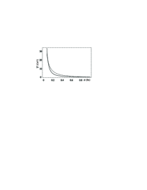
Figure 1: ${}^{1}P_{1}$ $np$ shallow potentials. $V_{7}$ (solid line) together with the Reid68 potential REID68 (dashed line).

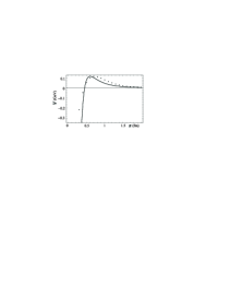
Figure 2: ${}^{1}P_{1}$ $np$ deep potentials. The full line corresponds to the potential which gives the correct effective range expansion (32) and the dots represent the Reid93 potential STOKS .

the level disappears and one gets the uniquely defined shallow representative of the family of isophase potentials, denoted by $V_{7}$. Fig. 1 shows this potential from which the centrifugal term has been subtracted. The potential $V_{7}$, is quite close to the Reid68 potential REID68 , represented in the same figure. Figure 2 shows one of the deep isophase potentials corresponding to $B_{3}/A_{3}=0.351$. This constant has been adjusted to get a potential as close as possible to Reid93 STOKS in the interval $0.4$ fm $\leq x\leq 2$ fm. This deep potential possesses a Pauli forbidden state of energy $E=-a_{3}^{2}=-44.46$ MeV. Contrary to the Reid93 potential which is deep but finite, our potential behaves at origin as $-2/x^{2}$. If necessary, it can be regularized as for example in Ref. SPAR .

It would be interesting to analyze the asymptotic behavior of our calculated potential to see if it is compatible with modern phenomenological potentials constructed in the spirit of meson theory, i.e. which include one-pion-exchange (OPE) contributions. This is precisely the case of the Reid93 potential, which includes OPE with neutral and charged pions (for details see Ref. STOKS ). The comparison given in Figure 3 shows that the shallow potential $V_{7}$ and its deep partner are practically identical in the asymptotic region and that they are both extremely close to the asymptotic form of the updated Reid93 potential MART . Thus our potentials are in the excellent agreement with expectations from Yukawa’s OPE theory. We remind that we subtracted the centrifugal barrier from our potentials in order to make this comparison feasible. In solving the Schrödinger equation this should be added back to the nucleon-nucleon interaction in each case. The fact that the shallow and deep potentials are asymptotically the same is physically correct. As mentioned in the introduction, deep potentials reflect the compositeness (quark structure) of the interacting particles in the overlap region but, once the particles are well separated, they could be treated as point particles as in OPE theories, which means that beyond some distance the deep and shallow potentials should coincide.

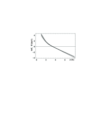
Figure 3: Asymptotic behavior in natural logarithmic scale of the value of the ${}^{1}P_{1}$ $np$ potentials. The full line represents our shallow potential of Fig. 1, the dashed line our deep potential of Fig. 2 and the dotted line the updated MART phenomenological Reid93 STOKS potential, including one-pion exchange.

III.2 The case $\ell=2$.

Now we have to apply two subsequent transformations associated with functions corresponding to $E=0$ and then, as above, a subchain of $\ell$-fixed transformations. After the first transformation with the function $u_{0,1}=x+x_{0}$, the potential $V_{1}$ of (24) has $u=1/(x+x_{0})$ and $\tilde{u}=(x+x_{0})^{2}$ as linearly independent solutions at $E=0$. Their linear combination $u_{0,2}=cu+\tilde{u}$, which is the transformation function for the second transformation step defined by the operator

$$L_{2}=-d/dx+u^{\prime}_{0,2}(x)/u_{0,2}(x)$$ (33)

contains two free parameters $x_{0}$ and $c$. These can be chosen such as the series expansion for $\tan\delta_{2}(k)$ starts at $k^{5}$. The intermediate (or background) potential

$$V_{2}=-2[\ln~{}u_{0,2}(x)u_{0,1}(x)]\,^{\prime\prime}=\frac{6(x+x_{0})[(x+x_{0})^{3}-2c]}{[c+(x+x_{0})^{3}]^{2}}$$ (34)

obtained from the $L=L_{2}L_{1}$ Darboux transformation (for more details see SS ) plays now the role of the initial potential for an $\ell$-fixed subchain of transformations. The background phase shift (modulo $\pi$) corresponding to $V_{2}$ is

$$\delta_{2}^{2}=\arctan\frac{3kx_{0}^{2}}{3x_{0}-k^{2}(x_{0}^{3}+c)}~{}.$$ (35)

Note that the function $\varphi_{2}(x,k)=L_{2}L_{1}\sin(kx+\delta_{2}^{2})$ is regular at the origin and describes an unnormalized scattering state for $\ell=2$. In the formula (22) we have to identify $\delta^{\ell}_{\ell}(k)$ with $\delta_{2}^{2}(k)$ of (35). After expanding in power series all arc tangent functions we find that the coefficient of the term linear in $k$ vanishes for $x_{0}$ given by (28) and

$$c={\textstyle\frac{1}{3}}\,[\,\sum\limits_{j\,=1}^{n}(a_{j}^{-3}+b_{j}^{-3})\,]\,$$ (36)

ensures the cancellation of the coefficient of $k^{3}$ in the series expansion of $\tan\delta^{N}_{2}$. Now, to find solutions of the free particle equations, giving rise to the regular family of the potential (34), to be used in (12), we need eigenfunctions of $h_{0}=-d^{2}/dx^{2}$ satisfying the condition $L_{2}L_{1}\psi_{j}(x,-ib_{j})=0$ at $x=0$. They are given by the following linear combination of exponentials

$$\psi_{j}(x,-ib_{j}) = [\,3x_{0}+3b_{j}x_{0}^{2}+b^{2}_{j}(c+x_{0}^{3})\,]\exp(b_{j}x)$$

$$- [\,3x_{0}-3b_{j}x_{0}^{2}+b^{2}_{j}(c+x_{0}^{3})\,]\exp(-b_{j}x)\,.$$

The irregular family still results from (30) subject to the condition that the ratio $B_{j}/A_{j}$ is different from that presented in (III.2).

With a fit of a similar quality to that performed for ${}^{1}P_{1}$ we could reproduce the ${}^{1}D_{2}$ partial wave phase shift of STOKS with the following four poles of the $S$-matrix

$$\begin{array}[]{l}a_{1}=-0.2047,\ \ a_{2}=-1.9800\\ b_{1}=\hphantom{-}1.2305,\ \ \ b_{2}=\hphantom{-}4.9631\end{array}$$ (38)

in fm^-1 units. From Eqs. (28) and (36) we get $x_{0}=-4.375$ fm, $c=116.08$ fm³. This leads to the following effective range expansion

$$k^{5}\cot\delta^{6}_{2}(k)=0.4496+10.9878k^{2}+\ldots\,.$$ (39)

where the superscript $N=6$ represents 4 transformation functions associated with the poles (38) plus two zero-eigenvalue functions $u_{0,1}$ and $u_{0,2}$ defined above. This is consistent with the formula (21) with $n=2$, $\nu=0$ and $\ell=2$. From the expansion (39) one can extract the scattering length $a_{02}$ and the effective range $r_{02}$ defined in Eq. (1). These values are shown in Table 2. They are comparable to those obtained for the potential Reid93 MART .

IV Conclusions

By working out these two particular cases we have shown that a new insight emerges into the role of the angular momentum of a central potential. If associated with the long-distance behavior of the potential, it allows us to introduce transformations that bring $\ell$ free parameters in the background phase shift (Eqs (27) and (35)). When a correct effective range expansion is required, each extra unit of angular momentum imposes a new constraint on the whole system of parameters of the model such as the number of constraints coincides with the number of parameters in the background phase shift. For the particular cases of $\ell=1$ and $\ell=2$ explicit solutions of the constraint equations are given. Thus, the extension of the method to $\ell>2$ is straightforward.

Before ending we should mention that the generalized Levinson theorem SWAN is always satisfied in our approach.

We are grateful to Mart Rentemeester for useful correspondence. B.F.S. acknowledges support from the Spanish Ministerio de Education, Cultura y Deporte Grant SAB2000-0240 and the Spanish MCYT and European FEDER grant BFM2002-03773. He is also grateful for hospitality at the Fundamental Theoretical Physics Laboratory of the University of Liege.

References

- (1) S. Saito, Prog. Theor. Phys. 41, 705 (1969).
- (2) E. Witten, Nucl. Phys. B188, 51 (1981).
- (3) C. V. Sukumar, J. Phys. A 18, 2917 (1985); 18, 2937 (1985).
- (4) J. -M. Sparenberg and D. Baye, Phys. Rev. C 55, 2175 (1997); J. -M. Sparenberg, D. Baye and H. Leeb, Phys. Rev. C 61, 024605 (2000).
- (5) H. Leeb and D. Leidinger, Few-Body Syst. Suppl. 6, 117 (1992); R. M. Adam, H. Fiedeldey, S. A. Sofianos and H. Leeb, Nucl. Phys. A559, 157 (1993).
- (6) B. F. Samsonov and Fl. Stancu, Phys. Rev. C 66, 034001 (2002).
- (7) J. -M. Sparenberg, Phys. Rev. Lett. 85, 2661 (2000).
- (8) P. Swan, Nucl. Phys. 46, 669 1963.
- (9) R. G. Newton Scattering theory of waves and particles, McGraw-Hill, New York, 1966.
- (10) M. N. Crum, Quarterly J. Math 6, 121 (1955).
- (11) L.D. Faddeev, Uspehi Mat. Nauk, 14, No 4 (88), 57 (1959); B.M. Levitan, Inverse Sturm-Liouville problems, (Nauka, Moscow, 1984).
- (12) R. V. Reid, Jr., Ann. Phys. (N.Y.) 50, 411 (1968).
- (13) V. G. J. Stoks, R. A. M. Klomp, C. P. F. Terheggen and J. J. de Swart, Phys. Rev. C49, 2950 (1994); for an updated data base and Reid93 potential see http://nn-online.sci.kun.nl.
- (14) M. N. Nagels, T. A. Rijken and J. J. de Swart, in Lecture Notes in Physics, vol. 82, Few-Body Systems and Nuclear Forces I, eds. H. Zingl, M. Haftel and H. Zankel (Springer, Berlin, 1878), p.17
- (15) M. Rentmeester, private communication
- (16) L. Mathelitsch and B. J. VerWest, Phys. Rev. C29, 739 (1984).