TUM/T39-02-14

ECT*-02-17

Bound state kinetics in high-energy nuclear collisions

Abstract

A Lorentz covariant kinetic equation for bound states and their constituents is presented and solved exactly in closed form. It describes in a unified way dynamical formation and dissociation of states such as quarkonia and (anti)-deuterons in the excited medium formed with a high-energy heavy-ion collision.

The possibility to describe hadronic bound states in strongly interacting matter provides an important tool for understanding the dynamics of the medium produced in high-energy heavy-ion collisions. The main reason lies in the fact that bound states can be formed and destroyed during specific stages of evolution of the medium, with a delicate interplay among various elements: the binding energy and structure of the object under consideration, the medium nature and characteristics which change as function of time and the abundances and phase-space correlations of the bound state constituents.

There are essentially two important kinds of bound states which deserve attention: heavy quarkonia ($J/\psi$, $\Upsilon$ and excited states) and (anti-)deuterons ($d$, $\bar{d}$). Their properties are quite different from one another and for this reason they probe different stages of a nuclear collision. The former are tightly bound, small objects, in general characterized by a hard scale and subject to confinement. They probe the early stages of a collision, in particular a possible quark-gluon plasma (QGP). The latter are very loosely bound, large objects which can be formed and survive dissociation only at the very latest moments of a collision. They probe the freeze-out stage.

Despite the aforementioned differences, the essential physics which regulates the time evolution in an interacting medium is very similar. For both bound states it is possible that they are formed in the evolving medium and are subsequently dissociated. How this happens is regulated by transition probabilities and by the medium constituents’ phase-space density. It is therefore desirable to have a unified description of these phenomena.

In the following we discuss a general kinetic equation, appropriate for both cases, and we present in closed form the exact solution, examining in detail specific features of the two cases under study. The solution is constructed for two different ways of specifying the initial condition. Finally, we discuss a simple analytical example, leaving the more realistic cases for future numerical calculations.

We begin by specifying the processes $B(p)+n(k)\leftrightarrow c_{1}(q_{1})+\bar{c}_{2}(q_{2})$ of dissociation and formation of a bound state $B$ into and from a pair of constituents $c_{1}c_{2}$ by means of a fourth degree of freedom labelled $n$. The corresponding momenta are indicated in parentheses. As mentioned earlier, the bound state $B$ can be a quarkonium or a(n) (anti-)deuteron, while the respective constituents are $q\bar{q}$ pairs of heavy quarks or proton-neutron $pn$ pairs. In particular, the dominant reactions to be considered are $c\bar{c}\leftrightarrow J/\psi g(\pi)$, $b\bar{b}\leftrightarrow\Upsilon g(\pi)$, $pn\leftrightarrow d\pi(\gamma)$, $\bar{p}\bar{n}\leftrightarrow\bar{d}\pi(\gamma)$. The amplitude for the process is illustrated in Fig. 1.

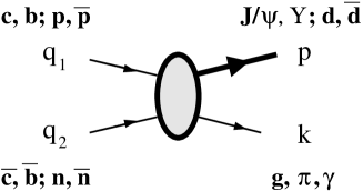
Figure 1: Diagram illustrating the amplitude for the formation of a bound state. The dissociation amplitude is obtained with detailed balance. Possible reactions are $c\bar{c}\leftrightarrow J/\psi g(\pi)$, $b\bar{b}\leftrightarrow\Upsilon g(\pi)$, $pn\leftrightarrow d\pi(\gamma)$, $\bar{p}\bar{n}\leftrightarrow\bar{d}\pi(\gamma)$

Borrowing concepts from the treatment of the non-linear Boltzmann equation GLW80 we postulate that the kinetic equation describing the time evolution of the phase-space density ${\cal F}_{B}$ of the bound state is then

$$p^{\mu}\partial_{\mu}\,{\cal F}_{B}(p,x)=C_{F}(p,x)-C_{D}(p,x)\,{\cal F}_{B}(p,x)\,,$$ (1)

consisting of a drift term (the differential operator $p^{\mu}\partial_{\mu}$) and a collision term, the latter made of a formation part

$$C_{F}(p,x)\! = \!\!\sum_{n}\int d\Phi(p,k,q_{1},q_{2})\ W_{c_{1}c_{2}\rightarrow Bn}(s,t)$$

$$\hskip 56.9055pt\times\ f_{c_{1}}(q_{1},x)f_{c_{2}}(q_{2},x)$$

and a dissociation part

$$C_{D}(p,x)=\sum_{n}\int d\Phi(p,k,q_{1},q_{2})\ W_{Bn\rightarrow c_{1}c_{2}}\ f_{n}(k,x)\,.$$ (3)

In the above $f_{c_{1}},f_{c_{2}}$ and $f_{n}$ are the phase-space distributions of the degrees of freedom participating in the collisions, depending implicitly on collision energy and centrality, while the phase-space integration measure is

$$d\Phi(p,k,q_{1},q_{2})\! = \!\frac{1}{2}\,\frac{d^{3}\vec{k}}{(2\pi)^{3}2E_{k}}\frac{d^{3}\vec{q}_{1}}{(2\pi)^{3}2E_{1}}\frac{d^{3}\vec{q}_{2}}{(2\pi)^{3}2E_{2}}$$

$$\times\ (2\pi)^{4}\delta^{4}(p\!+\!k\!-\!q_{1}\!-\!q_{2})\,.$$

As evident from the integration measure, all particles are assumed to be on their mass shell. The transition probability satisfies detailed balance as

$$W_{c_{1}c_{2}\rightarrow Bn}(s,t)=W_{Bn\rightarrow c_{1}c_{2}}(s,t)$$ (5)

and a sum over all particle species $n$ constituting the medium and contributing to dissociation and formation is indicated. Clearly, which degrees of freedom are active depends on the evolution time. The arguments of the transition probability are the Mandelstam variables $s=(p+k)^{2}=(q_{1}+q_{2})^{2}$ and $t=(q_{1}-p)^{2}=(k-q_{2})^{2}$. In the equations above we have neglected Bose-Einstein or Fermi-Dirac statistics, i.e. Bose enhancement and Pauli blocking.

All the dynamics is well defined once one specifies the distributions of the medium constituents and those of the bound state constituents, together with the transition probabilities $W_{c_{1}c_{2}\leftrightarrow Bn}$. The kinetic equation can then be solved in a closed form, which is convenient to present in two different ways, depending on how the initial condition is given, i.e. either at some initial global time $t_{0}$ or at some initial proper time $\tau_{0}$. The form of eq. (1) is very general and in the following we make no reference to the detailed structure of the collision term. In other words the functions $C_{F}$ and $C_{D}$ are assumed to be known.

When the initial condition is specified at some initial global time $t_{0}$ to be ${\cal F}_{B}^{0}(\vec{p},\vec{r})$, then the kinetic equation is conveniently re-written as

$$\left(\frac{\partial}{\partial t}+\vec{v}\cdot\frac{\partial}{\partial\vec{r}}\right)\,{\cal F}_{B}(\vec{p},\vec{r},t)\! = \!\lambda_{F}(\vec{p},\vec{r},t)$$

$$-\,\lambda_{D}(\vec{p},\vec{r},t)\ {\cal F}_{B}(\vec{p},\vec{r},t)\,,$$

where $\vec{v}=\vec{p}/E_{p}$ and $\lambda_{F,D}=C_{F,D}/E_{p}$. The solution to this last equation can be obtained with some simple steps. Neglecting the collision term, it is trivial to see that the solution is the scaled function

$${\cal F}_{B}^{*}(\vec{p},\vec{r},t)={\cal F}_{B}^{0}\left(\vec{p},\vec{\rho}(t-t_{0})\rule{0.0pt}{10.0pt}\right)\,,$$ (7)

where $\rho(t)=\vec{r}-\vec{v}\,t$. This is the case of free streaming. The case with dissociation but without formation was studied in BO89 to address the problem of charmonium suppression. There the solution was given as

$${\cal F}_{B}^{\rm diss}(\vec{p},\vec{r},t)\! = \!{\cal F}_{B}^{*}(\vec{p},\vec{r},t)$$

$$\times\ \exp\left[-\int_{t_{0}}^{t}\!dt^{\prime}\lambda_{D}\!\left(\,\vec{p},\vec{\rho}(t-t^{\prime}),t^{\prime}\rule{0.0pt}{10.0pt}\right)\right]\,.$$

Otherwise, with the only formation term and without dissociation, the solution is obtained by direct integration as

$${\cal F}_{B}^{\rm form}(\vec{p},\vec{r},t)={\cal F}_{B}^{*}(\vec{p},\vec{r},t)+\!\!\int_{t_{0}}^{t}\!\!\!dt^{\prime}\,\lambda_{F}\!\left(\,\vec{p},\vec{\rho}(t\!-\!t^{\prime}),t^{\prime}\rule{0.0pt}{10.0pt}\right)$$ (9)

It is interesting to notice the structure of the scaled argument $\vec{\rho}(t-t^{\prime})=\vec{r}-\vec{v}\,(t-t^{\prime})$, ensuring that any function of it is annihilated by the drift operator. This observation, although trivial, is crucial for the complete solution. We now combine the previous partial solutions and seek for the general case a solution of the form

$${\cal F}_{B}(\vec{p},\vec{r},t)\!\! = \!\!\!\left[{\cal F}_{B}^{*}(\vec{p},\vec{r},t)+\!\!\int_{t_{0}}^{t}\!\!dt^{\prime}\,\alpha\!\left(\,\vec{p},\vec{\rho}(t\!-\!t^{\prime}),t^{\prime}\rule{0.0pt}{10.0pt}\right)\right]$$

$$\ \ \times\ \exp\left[-\int_{t_{0}}^{t}\!dt^{\prime}\,\lambda_{D}\!\left(\,\vec{p},\vec{\rho}(t-t^{\prime}),t^{\prime}\rule{0.0pt}{10.0pt}\right)\right]\,,$$

where $\alpha$ is a function to be determined. With this choice, substituting in eq. (Bound state kinetics in high-energy nuclear collisions) one finds right away that the needed function is

$$\alpha(\vec{p},\vec{r},t)\!=\!\lambda_{F}(\vec{p},\vec{r},t)\,\exp\!\left[\int_{t_{0}}^{t}\!\!dt^{\prime}\lambda_{D}\!\left(\,\vec{p},\vec{\rho}(t\!-\!t^{\prime}),t^{\prime}\!\rule{0.0pt}{10.0pt}\right)\!\right]$$ (11)

Then, the general solution of the kinetic equation as function of global time can be obtained by substituting this last result into the trial form of eq. (Bound state kinetics in high-energy nuclear collisions). The final result is then

$${\cal F}_{B}(\vec{p},\vec{r},t)\! = \!\left\{\!\rule{0.0pt}{18.0pt}\right.{\cal F}_{B}^{*}(\vec{p},\vec{r},t)\ \exp\left[-\int_{t_{0}}^{t}\!dt^{\prime}\,\lambda_{D}\!\left(\,\vec{p},\vec{\rho}(t-t^{\prime}),t^{\prime}\rule{0.0pt}{10.0pt}\right)\right]$$

$$\left.\ \ +\,\int_{t_{0}}^{t}\!dt^{\prime}\,\lambda_{F}\!\left(\,\vec{p},\vec{\rho}(t-t^{\prime}),t^{\prime}\rule{0.0pt}{10.0pt}\right)\ \exp\left[-\int_{t^{\prime}}^{t}\!dt^{\prime\prime}\,\lambda_{D}\!\left(\,\vec{p},\vec{\rho}(t-t^{\prime\prime}),t^{\prime\prime}\rule{0.0pt}{10.0pt}\right)\right]\right\}\,.$$

By immediate inspection one finds that the initial condition is satisfied at $t=t_{0}$ and that the two previous partial solutions ${\cal F}_{B}^{\rm diss}$ in eq. (Bound state kinetics in high-energy nuclear collisions) and ${\cal F}_{B}^{\rm form}$ in eq. (9) are obtained in the respective limiting cases $\lambda_{F}=0$ and $\lambda_{D}=0$. We will comment on the obtained result later on, after the second derivation of the solution

Before we continue note that integrating over the position variables gives the invariant spectrum

$$E_{p}\frac{dN_{B}}{d^{3}\vec{p}}=\int\!\frac{d^{3}\vec{r}}{(2\pi)^{3}}\ {\cal F}_{B}(\vec{p},\vec{r},t_{f})$$ (13)

of the bound state at a given final global time $t_{f}$.

If the initial condition is specified at some initial proper time $\tau_{0}$ it is convenient to use momentum rapidity $y=1/2\,\log\left(\rule{0.0pt}{10.0pt}(E+p_{z})/(E-p_{z})\right)$ and space-time rapidity $\eta=1/2\,\log\left(\rule{0.0pt}{10.0pt}(t+z)/(t-z)\right)$ as longitudinal variables. The initial condition is then ${\cal F}_{B}^{0}(y,\vec{p}_{\perp},\eta,\vec{r}_{\perp})$. It is then useful to re-write the drift operator as $p^{\mu}\partial_{\mu}={\cal D}={\cal D}_{\parallel}+{\cal D}_{\perp}$ where

$${\cal D}_{\parallel}\!\! = \!\!m_{\perp}\left[\cosh(y-\eta)\,\frac{\partial}{\partial\tau}+\frac{1}{\tau}\,\sinh(y-\eta)\,\frac{\partial}{\partial\eta}\right]$$ (14)

$${\cal D}_{\perp}\!\!\! = \!\!\vec{p}_{\perp}\cdot\frac{\partial}{\partial\vec{r}_{\perp}}$$ (15)

As in the previous case, let us first consider the situation of free streaming, without a collision term. Neglecting the transverse coordinate dependence for a moment, the solution of the free streaming equation with the only operator ${\cal D}_{\parallel}$ is any function of the variable

$$\xi=\frac{\tau}{\tau_{0}}\sinh(y-\eta)\,,$$ (16)

It is therefore convenient to define the quantity

$$Y(\xi)=y-\log\left(\xi+\sqrt{1+\xi^{2}}\right)\,,$$ (17)

which reduces to $\eta$ when $\tau=\tau_{0}$. In this way one obtains the longitudinal free streaming solution

$${\cal F}_{B\parallel}^{*}(y,\eta,\tau)={\cal F}_{B\parallel}^{0}\left(y,Y(\xi)\rule{0.0pt}{10.0pt}\right)\,.$$ (18)

Concerning the transverse part we look for a scaling solution of the type

$${\cal F}_{B\perp}^{*}(\vec{r}_{\perp},\tau)={\cal F}_{B\perp}^{0}\left(\vec{r}_{\perp}-v_{\perp}\bar{\tau}\rule{0.0pt}{10.0pt}\right)\,,$$ (19)

with $v_{\perp}=p_{\perp}/m_{\perp}$ and $\bar{\tau}$ a function to be determined. The kinetic equation becomes

$${\cal D}{\cal F}_{B\perp}^{*} = \frac{\partial}{\partial\vec{r}_{\perp}}\,{\cal F}_{B\perp}^{*}\cdot(-v_{\perp})\ {\cal D}_{\parallel}\,\bar{\tau}+{\cal D}_{\perp}{\cal F}_{B\perp}^{*}$$

$$= {\cal D}_{\perp}{\cal F}_{B\perp}^{*}\cdot\left(1-\frac{{\cal D}_{\parallel}\,\bar{\tau}}{m_{\perp}}\right)=0\,,$$

which is equivalent, in the non-trivial case ${\cal D}_{\perp}{\cal F}_{B\perp}^{*}\neq 0$, to the equation ${\cal D}_{\parallel}\,\bar{\tau}=m_{\perp}$. It is simple to see that the solution is

$$\bar{\tau}(\xi,\tau)=\int_{\tau_{0}}^{\tau}\!d\tau^{\prime}\ \frac{1}{\sqrt{1+(\xi\tau_{0}/\tau^{\prime})^{2}}}$$ (21)

with the correct boundary condition $\bar{\tau}=0$ when $\tau=\tau_{0}$. The full free streaming solution is obtained by putting together the separate results for the longitudinal and transverse parts, yielding

$${\cal F}_{B}^{*}(y,\vec{p}_{\perp},\eta,\vec{r}_{\perp},\tau)={\cal F}_{B}^{0}\left(y,\vec{p}_{\perp},Y(\xi),\vec{\rho}_{\perp}(\xi,\tau)\rule{0.0pt}{10.0pt}\right)$$ (22)

being $\vec{\rho}_{\perp}(\xi,\tau)=\vec{r}_{\perp}-v_{\perp}\bar{\tau}(\xi,\tau)$. We now consider the more complicated case with dissociation, still neglecting formation. Analogously to the previous case, we look for a solution of the form

$${\cal F}_{B}^{\rm diss}(y,\vec{p}_{\perp},\eta,\vec{r}_{\perp},\tau)\! = \!{\cal F}_{B}^{*}(y,\vec{p}_{\perp},\eta,\vec{r}_{\perp},\tau)$$

$$\times\ \exp\left[-E(y,\vec{p}_{\perp},\eta,\vec{r}_{\perp},\tau)\rule{0.0pt}{10.0pt}\right]\,,$$

where the exponent $E$ is determined by the equation

$${\cal D}E(y,\vec{p}_{\perp},\eta,\vec{r}_{\perp},\tau)=C_{D}(y,\vec{p}_{\perp},\eta,\vec{r}_{\perp},\tau)\,.$$ (24)

The latter can be solved by direct integration, taking care of the fact that the integration measure should be the same as that of eq. (21), ensuring the correct scaling with the variable $\xi$. The solution is then

$$E(y,\vec{p}_{\perp},\eta,\vec{r}_{\perp},\tau)=\!\!\mbox{\Large$\displaystyle\int$}_{\!\!\!\!\!\tau_{0}}^{\tau}\!\!\!\!d\tau^{\prime}\frac{C_{D}\!\!\left(y,\vec{p}_{\perp},Y(\xi\tau_{0}/\tau^{\prime}),\vec{\rho}_{\perp}(\xi,\tau^{\prime})\rule{0.0pt}{10.0pt}\!\right)}{m_{\perp}\,\sqrt{1+(\xi\tau_{0}/\tau^{\prime})^{2}}}$$ (25)

With this last result, especially in its structure concerning the integration measure, it is now possible to obtain the full solution. Looking at the earlier solution given with eq. (Bound state kinetics in high-energy nuclear collisions) in the previous case of initialization at fixed global time, one can repeat the arguments leading to it and obtain, after defining the rates $\Lambda_{F,D}=C_{F,D}/m_{\perp}$ for dimensional clarity ($[\Lambda_{F,D}]=$ fm^-1), the general solution of the kinetic equation as

$${\cal F}_{B}(y,\vec{p}_{\perp},\eta,\vec{r}_{\perp},\tau)\!\! = \!\!\left\{\rule{0.0pt}{18.0pt}{\cal F}_{B}^{*}(y,\vec{p}_{\perp},\eta,\vec{r}_{\perp},\tau)\ \exp\!\left[-\mbox{\Large$\displaystyle\int$}_{\!\!\!\!\!\tau_{0}}^{\tau}\!\!d\tau^{\prime}\ \frac{\Lambda_{D}\left(y,\vec{p}_{\perp},Y(\xi\tau_{0}/\tau^{\prime}),\vec{\rho}_{\perp}(\xi,\tau^{\prime})\rule{0.0pt}{10.0pt}\right)}{\sqrt{1+(\xi\tau_{0}/\tau^{\prime})^{2}}}\right]\right.$$

$$\ \,+\!\!\left.\mbox{\Large$\displaystyle\int$}_{\!\!\!\!\!\tau_{0}}^{\tau}\!\!\!d\tau^{\prime}\ \frac{\Lambda_{F}\left(y,\vec{p}_{\perp},Y(\xi\tau_{0}/\tau^{\prime}),\vec{\rho}_{\perp}(\xi,\tau^{\prime})\rule{0.0pt}{10.0pt}\right)}{\sqrt{1+(\xi\tau_{0}/\tau^{\prime})^{2}}}\ \exp\!\left[-\mbox{\Large$\displaystyle\int$}_{\!\!\!\!\!\tau^{\prime}}^{\tau}\!\!\!\!d\tau^{\prime\prime}\ \frac{\Lambda_{D}\left(y,\vec{p}_{\perp},Y(\xi\tau_{0}/\tau^{\prime\prime}),\vec{\rho}_{\perp}(\xi,\tau^{\prime\prime})\rule{0.0pt}{10.0pt}\right)}{\sqrt{1+(\xi\tau_{0}/\tau^{\prime\prime})^{2}}}\right]\!\right\}.$$

In this case the initial condition is satisfied at $\tau=\tau_{0}$ and the partial solutions ${\cal F}_{B}^{\rm diss}$ and ${\cal F}_{B}^{\rm form}$ are again recovered in the respective limiting cases $\Lambda_{F}=0$ and $\Lambda_{D}=0$.

The structure of the solution is rich of details on the dynamics of dissociation and formation. The first part of the r.h.s. of eq. (Bound state kinetics in high-energy nuclear collisions), but see also eq. (Bound state kinetics in high-energy nuclear collisions), gives the final phase-space density of those bound states which were initially present at the start of the evolution at $\tau=\tau_{0}$. This term is especially important for the study of quarkonia. These are initially produced by hard collisions when the two nuclei first interact and are subsequently dissociated by the formed medium. On the other hand, at the high collision energies considered, (anti-)deuterons are absent at any early stage of a heavy-ion collision, therefore this term can be neglected. The second piece of the solution describes formation of bound states from $\tau_{0}$ up to $\tau^{\prime}$ and their subsequent dissociation from $\tau^{\prime}$ until $\tau$. For quarkonia it describes formation in a QGP, process that might be significant when the phase-space occupation of heavy quarks is large enough. This might happen at high collision energies, as recently suggested BMS00 ; TSR01 . For (anti-)deuterons this second term is the relevant one, describing coalescence of $pn$ pairs. This process is relevant only at low enough medium densities (small $\Lambda_{D}$), i.e. at the freeze-out stage. A more sophisticated treatment of this problem for deuterons at low and intermediate collision energies was developed in DB91 . Here, since we consider the high-energy collision regime, we can safely neglect many-body correlations. Hence the problem is significantly simpler.

An interesting application of eq. (Bound state kinetics in high-energy nuclear collisions) for the study of quarkonia is the comprehensive analysis of rapidity KPH01 and transverse momentum HZ02 dependencies of medium effects on the final spectrum. Regarding (anti-)deuterons, collective flow patterns emerge naturally as they are built-in both in formation and dissociation rates, providing a useful probe of the freeze-out properties of the produced medium M99 . Details of how different effects play a role both for quarkonia and for (anti-)deuterons can only be addressed with sufficiently realistic numerical studies. In fact, a detailed knowledge of the medium constituents’ and of the transition probabilities is required. In the following we will limit our discussion to a simple example to clarify the physical content of the result contained in eq. (Bound state kinetics in high-energy nuclear collisions).

Before doing so we recall that the invariant spectrum of bound states can be computed by means of the Cooper-Frye formula CF74 . Given a hyper-surface $\tau_{f}=\tau_{f}(\eta,\vec{r}_{\perp})$, one has

$$\frac{dN_{B}}{dy\,d^{2}\vec{p}_{\perp}}=\int_{\tau_{f}}\!\frac{d\sigma_{\mu}p^{\mu}}{(2\pi)^{3}}\ {\cal F}_{B}\left(y,\vec{p}_{\perp},\eta,\vec{r}_{\perp},\tau_{f}(\eta,\vec{r}_{\perp})\rule{0.0pt}{10.0pt}\right)$$ (27)

where ${\cal F}_{B}$ is given by eq. (Bound state kinetics in high-energy nuclear collisions) and

$$d\sigma_{\mu}p^{\mu}\! =\! d^{2}\vec{r}_{\perp}d\eta\,\left[\tau_{f}\,m_{\perp}\cosh(y-\eta)\rule{0.0pt}{12.0pt}\right.$$

$$\left.\hskip 28.45274pt-\ \tau_{f}\,\vec{p}_{\perp}\cdot\frac{\partial\tau_{f}}{\partial\vec{r}_{\perp}}-m_{\perp}\frac{\partial\tau_{f}}{\partial\eta}\sinh(y-\eta)\right]$$

is the invariant volume integration measure.

To discuss the physical content of the solution given with eq. (Bound state kinetics in high-energy nuclear collisions), or equivalently with eq. (Bound state kinetics in high-energy nuclear collisions), we focus on a single aspect of it. We refrain from discussing the part describing dissociation of initially present bound states. This was extensively done in BO89 for charmonium and only specific models of the medium can give qualitatively new answers. On the other hand the part describing formation deserves more attention. As mentioned earlier it can potentially account for quarkonium formation in a QGP, as suggested in TSR01 and become the dominant mechanism of production at high enough energies (RHIC, LHC). Moreover, the second term should describe formation of (anti-)deuterons in the late stages of the collision. While much work has been done in this domain, efforts were limited to applications of the coalescence model at freeze-out (See PBM98 ; SH99 for some recent results). Only recently ISZ03 a new attempt was made to address this problem.

Therefore, focussing attention on bound state formation in the medium, we neglect the first term in eq. (Bound state kinetics in high-energy nuclear collisions) either because dissociation destroys all the initially present bound states or because there are no bound states to start with. With significant simplifications of the solution in order to follow the essential physics, we neglect all dependencies on $y,\vec{p}_{\perp},\eta$ and $\vec{r}_{\perp}$. The remaining solution can be written as

$$N_{B}(\tau)=\int_{\tau_{0}}^{\tau}\!\!d\tau^{\prime}\,\Lambda_{F}(\tau^{\prime})\,\exp\left[-\int_{\tau^{\prime}}^{\tau}\!\!d\tau^{\prime\prime}\,\Lambda_{D}(\tau^{\prime\prime})\right]\,.$$ (29)

This situation is equivalent to having solved the first order ordinary differential equation $dN_{B}/d\tau=\Lambda_{F}-\Lambda_{D}\,N_{B}$ with initial condition $N_{B}^{0}=0$. We then assume that the time dependence of the formation and dissociation rates are

$$\Lambda_{F}(\tau)=\frac{P_{F}\,N_{c_{1}}N_{c_{2}}}{\tau}\ \ \ \ \ {\rm and}\ \ \ \ \ \Lambda_{D}(\tau)=\frac{P_{D}\,N_{D}}{\tau}\,,$$ (30)

where $P_{F,D}$ are formation and dissociation probabilities, $N_{c_{1,2}}$ indicates the number of particles which can form the bound state (either $pn$ or $q\bar{q}$ pairs) and $N_{D}$ is the number of particles that can dissociate the bound state. With the latter assumption one can readily perform the time integrations in eq. (29) obtaining the final number of bound states at $\tau_{f}$ as

$$N^{f}_{B}=\frac{P_{F}\,N_{c_{1}}N_{c_{2}}}{P_{D}\,N_{D}}\,\left[1-\left(\tau_{0}/\tau_{f}\right)^{P_{D}N_{D}}\right]\propto\frac{N_{c_{1}}N_{c_{2}}}{N_{D}}$$ (31)

when $P_{D}N_{D}\gg 1$. This last results indicates that the final yield is proportional to the number of particles which can form the bound state and inversely proportional to the number of particles that can dissociate it. With the help of numerical simulations, the consequences of this scaling law for deuterons were discussed previously in SNK95 . Moreover, since the number of dissociating particles is proportional to the volume of the medium, either at hadronization for quarkonia or at freeze-out for (anti-)deuterons, we recover the well known coalescence formula CK86 , here newly obtained with dynamical considerations. The above simplified derivation gives some insight in the coupled dynamics of dissociation and formation. In particular, as discussed in GKMSG02 ; T03 ; GG99 , the experimental observation of an inverse proportionality of the number of quarkonia with the total number of produced hadrons, might give support to this new mechanism of production in a QGP.

We can now conclude by summarizing the results presented above. The aim of this paper has been twofold: to present a unified theoretical description of bound state formation in the strongly interacting medium, formed with a heavy-ion collision at high energy, and to provide a useful tool to be applied in numerical calculations of bound state spectra. This was achieved by means of a kinetic equation with a collision term consisting of formation and dissociation parts. The equation was solved exactly in closed form and the result given in eqs. (Bound state kinetics in high-energy nuclear collisions) and (Bound state kinetics in high-energy nuclear collisions).

The physical content of the solution was discussed and a simplified version of it was given with eq. (31) in order to illustrate that the yield of bound states form in the medium satisfy the scaling embedded in the coalsecence formula, i.e. direct proportionality with the number of bound state constituents and inverse proportionality with the system volume. The full solution, on the other hand, provides a convenient tool for future numerical studies, which require quantitative knowledge of the phase-space distributions of the degrees of freedom involved and of the transition probabilities among those degrees of freedom.

References

- (1) S. de Groot, W. van Leeuwen and Ch. van Weert, Relativistic Kinetic Theory, North-Holland, Amsterdam, 1980;
- (2) J. P. Blaizot and J. Y. Ollitrault, Phys. Rev. D 39 (1989) 232;
- (3) P. Braun-Munzinger and J. Stachel, Phys. Lett. B 490 (2000) 196;
- (4) R. Thews, M. Schroedter and J. Rafelski, Phys. Rev. C 63 (2001) 054905;
- (5) B. Kopeliovich, A. Polleri and J. Hüfner, Phys. Rev. Lett. 87 (2001) 112302;
- (6) J. Hüfner and P. f. Zhuang, arXiv:nucl-th/0208004;
- (7) B. Monreal et al., Phys. Rev. C 60 (1999) 051902;
- (8) F. Cooper and G. Frye, Phys. Rev. D 10 (1974) 186;
- (9) P. Danielewicz and G. Bertsch, Nucl. Phys. A 533 (1991) 712;
- (10) A. Polleri, J. Bondorf and I. Mishustin, Phys. Lett. B 419 (1998) 19;
- (11) R. Scheibl and U. Heinz, Phys. Rev. C 59 (1999) 1585;
- (12) B. Ioffe, I. Shushpanov and K. Zyablyuk, arXiv:hep-ph/0302052;
- (13) H. Sorge, J. Nagle and B. Kumar, Phys. Lett. B 355 (1995) 27;
- (14) L. Csernai and J. Kapusta, Phys. Rep. 131 (1986) 223 and references therein;
- (15) M. Gorenstein, A. Kostyuk, L. McLerran, H. Stocker and W. Greiner, J. Phys. G 28 (2002) 2151;
- (16) R. Thews, CERN Yellow report “Hard Probes in Heavy Ion Collisions at the LHC”, arXiv:hep-ph/0302050;
- (17) M. Gaździcki, Phys. Rev. C 60 (1999) 054903; M. Gaździcki and M. Gorenstein, Phys. Rev. Lett. 83 (1999) 4009.