Dynamical Model of Weak Pion Production Reactions

Abstract

The dynamical model of pion electroproduction developed in Physical Review C63, 055201 (2001) has been extended to investigate the weak pion production reactions. With the Conserved Vector Current(CVC) hypothesis, the weak vector currents are constructed from electromagnetic currents by isospin rotations. Guided by the effective chiral lagrangian method and using the unitary transformation method developed previously, the weak axial vector currents for $\pi$ production are constructed with no adjustable parameters. In particular, the N-$\Delta$ transitions at $Q^{2}\rightarrow 0$ are calculated from the constituent quark model and their $Q^{2}$-dependence is assumed to be identical to that determined in the study of pion electroproduction. The main feature of our approach is to renormalize these bare N-$\Delta$ form factors with the dynamical pion cloud effects originating from the non-resonant $\pi$ production mechanisms. The predicted cross sections of neutrino-induced pion production reactions, $N(\nu_{\mu},\mu^{-}\pi)N$, are in good agreement with the existing data. We show that the renormalized(dressed) axial N-$\Delta$ form factor contains large dynamical pion cloud effects and this renormalization effects are crucial in getting agreement with the data. We conclude that the N-$\Delta$ transitions predicted by the constituent quark model are consistent with the existing neutrino induced pion production data in the $\Delta$ region, contrary to the previous observations. This is consistent with our previous findings in the study of pion electroproduction reactions. However, more extensive and precise data of neutrino induced pion production reactions are needed to further test our model and to pin down the $Q^{2}$-dependence of the axial vector N-$\Delta$ transition form factor.

I INTRODUCTION

It is now well recognized that an important challenge in nuclear research is to understand the hadron structure within Quantum Chromodynamics(QCD). One of the important information for pursuing this research is the electromagnetic and weak N-$\Delta$ transition form factors. Such information are important for testing current hadron models and perhaps also Lattice QCD calculations in the near future. In particular, we can address the question about whether N and $\Delta$ are deformed. If they are deformed, is it due to the gluon interactions between quarks or due to the pion cloud which is resulted from the spontaneously breaking of the chiral symmetry of QCD?

As a step in this direction, we have developedsl1 ; sl2 in recent years a dynamical model for investigating the pion photoproduction and electroproduction reactions at energy near the $\Delta$ resonance. The dynamical approach, which has also been pursued by several groupstanabe ; yang ; nbl ; pearcelee ; afn ; surya ; ky1 ; ky2 , is different from the approaches based on either dispersion relationscgln ; hdt ; a98 or K-matrix methodmuko90 ; muko99 ; maid ; said in interpreting the data. In Refs.1 and 2, we not only have extracted the electromagnetic N-$\Delta$ transition form factors from the data, but also have provided an interpretation of the extracted parameters in terms of hadron model calculations. In particular, we have shown that including the dynamical pion cloud effect in theoretical analyses can resolve a long-standing puzzle that the N-$\Delta$ M1 transition form factor $G_{M}^{N\Delta}(0)$ predicted by the constituent quark model is about 40 $\%$ lower than the empirical value. Furthermore, the dynamical pion cloud is found to play an important role in determining the $Q^{2}$-dependence of $G_{M}^{N\Delta}(Q^{2})$ which drops faster than the proton form factor $G_{p}(Q^{2})$ as $Q^{2}$ increases. The predicted electric E2 and Coulomb C2 N-$\Delta$ transition form factors, which exhibit very pronounced meson cloud effects at low $Q^{2}$, have stimulated some experimental initiativesbern02 . Similar results were also obtained in Ref.ky2 .

Since weak currents are closely related to electromagnetic currents within the Standard Model, it is straightforward to extend our dynamical approach to study weak pion production reactions. In this paper, we report the progress we have made in this direction. Our objective is to develop a framework for extracting the axial vector N-$\Delta$ form factors from the data of neutrino-induced pion production reactions. In particular, we would like to explore whether a dynamical approach , as developed in our study of pion electroproduction, can also resolve a similar problem that the axial N-$\Delta$ transition strength calculatedhhm ; lmz from the constituent quark model is about 30 $\%$ lower than what was extracteddata90 from the data. We will also make predictions for future experimental tests which could be conducted at Fermi Lab, KEK and Japan Hadron Facility in the near future.

To introduce our model, it is necessary to first briefly review the dynamical approach developed in Ref.sl1 ; sl2 (called SL model). Our starting point is an interaction Hamiltonian $H_{I}=\Gamma_{MB\leftrightarrow B^{\prime}}$ which describes the absorption and emission of mesons($M$) by baryons($B$). In the SL model, such a Hamiltonian is obtained from phenomenological Lagrangians. In fact, the approach is more general and this Hamiltonian can be defined in terms of a hadron model, as attempted, for example, in Ref. yoshi , or by using the vertex functions predicted by Lattice QCD calculations.

It is a non-trivial many-body problem to calculate $\pi N$ scattering and $\gamma N\rightarrow\pi N$ reaction amplitudes from the interaction Hamiltonian $H_{I}=\Gamma_{MB\leftrightarrow B^{\prime}}$. To obtain a manageable reaction model, a unitary transformation methodsl1 ; ksh is used up to second order in $H_{I}$ to derive an effective Hamiltonian. The essential idea of the employed unitary transformation method is to eliminate the unphysical vertex interactions $MB\rightarrow B^{\prime}$ with $m_{M}+m_{B}<m_{B^{\prime}}$ from the Hamiltonian and absorb their effects into $MB\rightarrow M^{\prime}B^{\prime}$ two-body interactions. For the pion production processes in the $\Delta$ region, the resulting effective Hamiltonian is defined in a subspace spanned by the $\pi N$, $\gamma N$ and $\Delta$ states and has the following form

$$H_{eff} = H_{0}+v_{\pi N}+v_{\gamma\pi}+\Gamma_{\pi N\leftrightarrow\Delta}+\Gamma_{\gamma N\leftrightarrow\Delta},$$ (1)

where $v_{\pi N}$ is a non-resonant $\pi N$ potential, and $v_{\gamma\pi}$ describes the non-resonant $\gamma N\leftrightarrow\pi N$ transition. The $\Delta$ excitation is described by the vertex interactions $\Gamma_{\gamma N\leftrightarrow\Delta}$ for the $\gamma N\leftrightarrow\Delta$ transition and $\Gamma_{\pi N\leftrightarrow\Delta}$ for the $\pi N\leftrightarrow\Delta$ transition. The non-resonant $v_{\gamma\pi}$ consists of the usual pseudo-vector Born terms, $\rho$ and $\omega$ exchanges, and the crossed $\Delta$ term.

From the effective Hamiltonian Eq. (1), it is straightforward to derive a set of coupled equations for $\pi N$ and $\gamma N$ reactions. The resulting pion photoproduction amplitude can be written as

$$T_{\gamma\pi}(E)=t_{\gamma\pi}(E)+\frac{\bar{\Gamma}_{\Delta\rightarrow\pi N}(E)\bar{\Gamma}_{\gamma N\rightarrow\Delta}(E)}{E-m_{\Delta}-\Sigma_{\Delta}(E)}.$$ (2)

The non-resonant amplitude $t_{\gamma\pi}$ is calculated from $v_{\gamma\pi}$ by

$$t_{\gamma\pi}(E)=v_{\gamma\pi}+t_{\pi N}(E)G_{\pi N}(E)v_{\gamma\pi},$$ (3)

where $G_{\pi N}$ is the $\pi N$ free propagator, and $t_{\pi N}$ is calculated from the non-resonant $\pi N$ interaction $v_{\pi N}$.

The dressed vertices in Eq. (2) are defined by

$$\bar{\Gamma}_{\gamma N\rightarrow\Delta}(E) = \Gamma_{\gamma N\rightarrow\Delta}+v_{\gamma\pi}G_{\pi N}(E)\bar{\Gamma}_{\pi N\rightarrow\Delta}(E),$$ (4)

$$\bar{\Gamma}_{\Delta\rightarrow\pi N}(E) = [1+t_{\pi N}(E)G_{\pi N}(E)]\Gamma_{\Delta\rightarrow\pi N}.$$ (5)

The $\Delta$ self-energy in Eq. (2) is then calculated from

$$\Sigma_{\Delta}(E)=\Gamma_{\pi N\rightarrow\Delta}G_{\pi N}(E)\bar{\Gamma}_{\Delta\rightarrow\pi N}(E).$$ (6)

As seen in the above equations, an important feature of the dynamical model is that the bare vertex $\Gamma_{\gamma N\rightarrow\Delta}$ is modified by the non-resonant interaction $v_{\gamma\pi}$ to give the dressed vertex $\bar{\Gamma}_{\gamma N\rightarrow\Delta}$, as defined by Eq. (4). The second terms in the right-hand sides of Eqs. (4) and (5) can be interpreted as the $dynamical$ pion cloud effects on the N-$\Delta$ transitions. We can then identify the parameters of the bare vertex $\Gamma_{\gamma N\rightarrow\Delta}$ with the predictions from hadron models within which the $\pi$-baryon states in $continuum$ are excluded. Such a separation of the reaction mechanisms from the excitations of hadron internal structure is an essential ingredient of a dynamical approach, but is not an objective of the approaches based on either dispersion relationscgln ; hdt ; a98 or K-matrix methodmuko90 ; muko99 ; maid ; said .

In the above formulation, the matrix elements $v_{\gamma\pi}$ and $\Gamma_{\gamma N\leftrightarrow\Delta}$ are determined by the electromagnetic current $J^{em}_{\mu}$. The dynamical formulation for investigating weak pion production reactions can be obtained from Eqs. (1)-(6) by replacing $J^{em}_{\mu}$ by $V_{\mu}-A_{\mu}$, where $V_{\mu}$ and $A_{\mu}$ are the weak vector and axial vector currents respectively. By Conserved Vector Current(CVC) relations, the vector currents $V_{\mu}$ can be obtained from the electromagnetic currents by isospin rotations. Guided by the effective chiral Lagrangian method and using the similar procedures of the SL model, we can construct the axial vector currents $A_{\mu}$ for pion production reactions. The resulting axial current amplitude consists of nucleon-Born, rho-exchange, pion-pole, and $\Delta$ excitation terms and can be calculated using the parameters in the literatures. In particular, the bare axial N-$\Delta$ transitions at $Q^{2}\rightarrow 0$ are assumed to be those calculated by Hemmert, Holstein, and Mukhopadhyayhhm within the constituent quark model.

Most of the earlier theoretical investigationssalin ; adler ; bij ; zuker ; schr73 of weak pion production reactions were performed during the years around 1970. The model which was most often used in analyzing the data was developed by Adleradler . He considered a model based on the dispersion relations of Chew, Goldberger, Low, and Nambu(CGLN) cgln . The driving terms and subtraction terms of the dispersion relations are calculated from the nucleon Born terms. No vector meson exchanges are included. Additional subtraction terms are added to remove the kinematic singularities of multipole amplitudes. In solving the dispersion relation equations, only the $P_{33}$ phases are included to account for the unitarity condition via Watson Theorem and the imaginary parts of other multipole amplitudes are neglected. Clearly, Adler’s approach needs improvements for a precise extraction of the axial N-$\Delta$ from factors from the data. We however will not address this issue in this paper. Instead, we focus on the development of a dynamical approach outlined above.

In section II, we present a formulation for calculating the cross sections of neutrino induced pion production reactions. The current matrix elements needed for our calculations are given in section III. The results are presented in section IV. Conclusions and discussions on possible future developments will be given in section V.

II Cross Section Formula

The formula for calculating the cross sections of neutrino induced pion production reactions have been given in Ref.adler . In this section, we would like to present a different formulation which is more closely related to the commonly used formulation of pion electroproduction, and is more convenient for our calculations based on a dynamical formulation of the problem.

We focus on the $\nu+N\rightarrow l+\pi+N$ reaction, where $l$ stands for electron($e$) or muon($\mu)$ and $\nu$ for electron neutrino($\nu_{e}$) or muon neutrino($\nu_{\mu}$). We start with the interaction Lagrangian

$$L_{int}(x)=\frac{G_{F}\cos\theta_{c}}{\sqrt{2}}[l^{\mu}(x)J_{\mu}(x)+\mbox{h.c.}],$$ (7)

where $G_{F}=1.16637\times 10^{-5}$ (GeV)^-2, $cos\theta_{c}=0.974$,

$$l^{\mu}(x) = \bar{\psi}_{l}(x)\gamma^{\mu}(1-\gamma_{5})\psi_{\nu}(x)$$ (8)

is the lepton current and

$$J^{\mu}(x)=V^{\mu}(x)-A^{\mu}(x)$$ (9)

is the hadron current. The vector current($V^{\mu}$) and axial vector current($A^{\mu}$) will be constructed later in terms of hadronic degrees of freedom.

The coordinate system for calculating the differential cross sections of the $\nu(p_{\nu})+N(p)\rightarrow l(p_{l})+\pi(k)+N(p^{\prime})$ reaction is chosen such that the leptons are on the x-z plane. The momentum transfer $\bm{q}=\bm{p}_{\nu}-\bm{p}_{l}$, which is also the total momentum of the final $\pi N$ system in the laboratory system, is along the z-axis. The final $\pi N$ system forms a plane which has an angle $\phi_{\pi}$ with respect to the lepton $\nu$-$l$ plane. This choice is identical to that widely used in the study of pion electroproduction. It is then straightforward to show that the differential cross section can be written as

$$\frac{d\sigma^{5}}{dE_{l}d\Omega_{l}d\Omega_{\pi}^{*}}=\frac{G_{F}^{2}\cos^{2}\theta_{c}}{2}\frac{|\bm{p}_{l}|}{|\bm{p}_{\nu}|}\frac{|\bm{k}_{c}|m_{N}}{(2\pi)^{5}W}L^{\mu\nu}W_{\mu\nu},$$ (10)

where $m_{N}$ is the nucleon mass, and the phase space factor is expressed in terms of lepton momenta $\bm{p}_{l}$ and $\bm{p}_{\nu}$ in the laboratory(Lab) frame, pion momentum $\bm{k}_{c}$ in the $\pi N$ center of mass(C.M.) frame, and the invariant mass $W$ of the $\pi N$ subsystem. The angle $\Omega_{\pi}^{*}$ in Eq. (10) is the pion scattering angle defined in the $\pi N$ center of mass frame.

The lepton tensor in Eq. (10) is

$$L^{\mu\nu}=p^{\mu}_{l}p^{\nu}_{\nu}+p^{\nu}_{l}p^{\mu}_{\nu}-g^{\mu\nu}(p_{\nu}\cdot p_{l})\pm i\epsilon^{\alpha\beta\mu\nu}p_{\nu,\alpha}p_{l,\beta}.$$ (11)

Here $\epsilon^{0123}=1$ and $+(-)$ in the last term is for neutrino (anti-neutrino) reactions. The hadron tensor is

$$W_{\mu\nu}=\frac{1}{2}\sum_{s^{\prime}_{N}s_{N}}j_{\mu}j^{*}_{\nu},$$ (12)

where $j_{\mu}$ implicitly represents the matrix element

$$<k,p^{\prime}s_{N}^{\prime}\mid J_{\mu}\mid ps_{N}> = \frac{1}{(2\pi)^{3}}\sqrt{\frac{m_{N}^{2}}{2E_{\pi}(k)E_{N}(p^{\prime})E_{N}(p)}}j_{\mu}$$ (13)

with $s_{N}$ denoting the z-component of nucleon spin. Such a simplified notation for hadron current matrix element will be used in the rest of this paper.

To see the current non-conserving part of hadron current explicitly, we introduce the following variables

$$K^{\mu} = \frac{p^{\mu}_{\nu}+p^{\mu}_{l}}{2},$$ (14)

$$q^{\mu} = p^{\mu}_{\nu}-p^{\mu}_{l},$$ (15)

$$Q^{2} = -q^{2}=-m_{l}^{2}+2(p_{\nu}\cdot p_{l}),$$ (16)

where $q^{\mu}$ is the lepton momentum transfer and $m_{l}$ is the mass of lepton $l$. We then obtain

$$L^{\mu\nu}W_{\mu\nu} = \frac{1}{2}\sum_{s_{N}^{\prime},s_{N}}[2(K\cdot j)(K\cdot j^{*})-\frac{(q\cdot j)(q\cdot j^{*})}{2}-\frac{(j\cdot j^{*})(Q^{2}+m_{l}^{2})}{2}$$ (17)

$$\pm i\epsilon^{\alpha\beta\mu\nu}q_{\alpha}K_{\beta}j_{\mu}j_{\nu}^{*}].$$

The hadron current $j^{\mu}$ in Eq. (17) is defined in the Lab frame. To account for the final $\pi N$ interaction within the dynamical formulation and to get an expression in terms of the scattering angle $\Omega^{*}_{\pi}$ of Eq. (10), we need to write $j^{\mu}$ in terms of the current $j^{\mu}_{c}$ defined in the $\pi N$ C.M. frame. With the choice of the coordinate system described above, the transformation from the Lab frame to the $\pi N$ C.M. frame is just a Lorentz boost along the z-axis. For the x and y components of the hadron current, we obviously have the following simple relations

$$j^{x} = \cos\phi_{\pi}j_{c}^{x}-\sin\phi_{\pi}j_{c}^{y},$$ (18)

$$j^{y} = \sin\phi_{\pi}j_{c}^{x}+\cos\phi_{\pi}j_{c}^{y}.$$ (19)

For the z and time components, the transformation relations are

$$j^{0} = \cosh\alpha j_{c}^{0}+\sinh\alpha j_{c}^{z},$$ (20)

$$j^{z} = \sinh\alpha j_{c}^{0}+\cosh\alpha j_{c}^{z},$$ (21)

where

$$\cosh\alpha =\frac{E_{N,c}}{m_{N}} =\frac{m_{N}+\omega}{W},$$ (22)

$$\sinh\alpha =\frac{|\bm{q}_{c}|}{m_{N}} =\frac{|\bm{q}|}{W}.$$ (23)

Here we have introduced $q^{\mu}=(\omega,\bm{q})$ and $q^{\mu}_{c}=(\omega_{c},\bm{q}_{c})$ as the momentum transfers in the Lab and $\pi N$ C.M. frames respectively, and $E_{N,c}=\sqrt{\bm{q}^{2}_{c}+m_{N}^{2}}$.

Since the leptons are on the x-z plane and the momentum transfer $\bm{q}$ is in the z-axis, we obviously have

$$K^{x} = \frac{|\bm{p}_{\nu}||\bm{p}_{l}|}{|\bm{q}|}\sin\theta_{l},$$ (24)

$$K^{y} = 0,$$ (25)

$$K^{z} = \frac{|\bm{p}_{\nu}|^{2}-|\bm{p}_{l}|^{2}}{2|\bm{q}|},$$ (26)

$$K^{0} = \frac{|\bm{p}_{\nu}|+E_{l}}{2}.$$ (27)

In the above equations, $\theta_{l}$ is the angle between the outgoing lepton momentum $\bm{p}_{l}$ and the incident neutrino momentum $\bm{p}_{\nu}$.

By using the above relations Eqs. (18)-(27), it is straightforward, although tedious, to cast Eq. (17) into the following form

$$L^{\mu\nu}W_{\mu\nu} = \frac{1}{2}\sum_{s_{N}^{\prime},s_{N}}[R_{T}+R_{L}+R_{LT}\cos\phi_{\pi}+R_{TT}\cos 2\phi_{\pi}$$ (28)

$$+R_{LT^{\prime}}\sin\phi_{\pi}+R_{TT^{\prime}}\sin 2\phi_{\pi}]$$

All terms in the above equation can be calculated from $j^{\mu}_{c}$ defined in the $\pi N$ C.M. frame. Explicitly, $R_{T}$ and $R_{L}$ terms are given as

$$R_{T} = ((K^{x})^{2}+\frac{Q^{2}+m_{l}^{2}}{2})(|j^{x}_{c}|^{2}+|j^{y}_{c}|^{2})\mp x\mbox{Im}(j^{x}_{c}j^{y*}_{c}),$$ (29)

$$R_{L} = \frac{1}{2\bm{q}_{c}^{2}}[(x^{2}-Q^{4}-Q^{2}m_{l}^{2})|j^{0}_{c}|^{2}+2(xy-Q^{2}\omega_{c}-\omega_{c}m_{l}^{2})Re(j_{c}^{0}\rho^{*})$$ (30)

$$+(y^{2}-\omega_{c}^{2}+m_{l}^{2})|\rho|^{2}],$$

with

$$x = \frac{(E_{\nu}+E_{l})Q^{2}-\omega m_{l}^{2}}{|\bm{q}|},$$ (31)

$$y = \frac{(E_{\nu}+E_{l})\omega_{c}+\cosh\alpha\ m_{l}^{2}}{|\bm{q}|}.$$ (32)

In deriving Eq. (30), we have defined $\rho=q\cdot j=\omega_{c}j^{0}_{c}-|\bm{q}_{c}|j^{z}_{c}$ and eliminated $j^{z}_{c}$.

The other terms in Eq. (28) are given as

$$R_{LT} = \frac{2K^{x}}{|\bm{q}_{c}|}(-\mbox{Re}((xj^{0}_{c}+y\rho)j^{x*}_{c})\pm\mbox{Im}((Q^{2}j^{0}_{c}+\omega_{c}\rho)j^{y*}_{c}),$$ (33)

$$R_{TT} = (K^{x})^{2}(|j^{x}_{c}|^{2}-|j^{y}_{c}|^{2}),$$ (34)

$$R_{LT^{\prime}} = \frac{2K^{x}}{|\bm{q}_{c}|}(\mbox{Re}((xj^{0}_{c}+y\rho)j^{y*}_{c})\pm\mbox{Im}((Q^{2}j^{0}_{c}+\omega_{c}\rho)j^{x*}_{c}),$$ (35)

$$R_{TT^{\prime}} = -2(K^{x})^{2}\mbox{Re}(j^{x}_{c}j^{y*}_{c}).$$ (36)

It is interesting to note that in the $m_{l}=0$ limit the above formula become

$$R_{T} = \frac{Q^{2}}{1-\epsilon}[\frac{|j^{x}_{c}|^{2}+|j^{y}_{c}|^{2}}{2}\mp\sqrt{1-\epsilon^{2}}\mbox{Im}(j^{x}_{c}j^{y*}_{c})],$$ (37)

$$R_{L} = \frac{Q^{2}}{1-\epsilon}\epsilon\frac{Q^{2}}{|\bm{q}_{c}|^{2}}|\bar{j}_{c}^{0}|^{2},$$ (38)

$$R_{LT} = \frac{Q^{2}}{1-\epsilon}\sqrt{\frac{2\epsilon(1+\epsilon)Q^{2}}{|\bm{q}_{c}|^{2}}}{}[-\mbox{Re}(\bar{j}^{0}_{c}j^{x*}_{c})\pm\sqrt{\frac{1-\epsilon}{1+\epsilon}}\mbox{Im}(\bar{j}^{0}_{c}j^{y*}_{c})],$$ (39)

$$R_{TT} = \frac{Q^{2}}{1-\epsilon}[\frac{\epsilon(|j^{x}_{c}|^{2}-|j^{y}_{c}|^{2})}{2}],$$ (40)

$$R_{LT^{\prime}} = \frac{Q^{2}}{1-\epsilon}\sqrt{\frac{2\epsilon(1+\epsilon)Q^{2}}{|\bm{q}_{c}|^{2}}}{}[\mbox{Re}(\bar{j}^{0}_{c}j^{y*}_{c})\pm\sqrt{\frac{1-\epsilon}{1+\epsilon}}\mbox{Im}(\bar{j}^{0}_{c}j^{x*}_{c})],$$ (41)

$$R_{TT^{\prime}} = \frac{Q^{2}}{1-\epsilon}[-\epsilon\mbox{Re}(j^{x}_{c}j^{y*}_{c})],$$ (42)

where

$$\epsilon=\frac{1}{1+\frac{2\mid\bm{q}\mid^{2}}{Q^{2}}\tan^{2}\frac{\theta_{l}}{2}}$$ (43)

with $\bar{j}_{c}^{0}=j_{c}^{0}+\omega_{c}\rho/Q^{2}$. Eqs. (37)-(43) are very similar to the familiar forms of pion electroproduction. In the energy region we are considering, the muon mass cannot be neglected. Calculations of the differential cross section Eq. (10) for the $\nu_{\mu}+N\rightarrow\mu+\pi+N$ reactions must be done by using Eqs. (29)-(36).

To deal with the old data, we need to calculate the differential cross section in terms of the variables $W$(invariant mass of $\pi N$ subsystem), $Q^{2}=-q^{2}$(Eq. (16)) instead of lepton energy ($E_{l}$) and scattering angle $\theta_{l}$. The relation between them are

$$Q^{2} = 2E_{\nu}E_{l}-2|\bm{p}_{l}||\bm{p}_{\nu}|\cos\theta_{l}-m_{l}^{2},$$ (44)

$$W = \sqrt{m_{N}^{2}+2m_{N}(E_{\nu}-E_{l})-Q^{2}}.$$ (45)

By using the above relations, we can obtain the following relation

$$\frac{d\sigma}{dWdQ^{2}d\Omega^{*}_{\pi}} = \frac{2\pi W}{2m_{N}|\bm{p}_{\nu}||\bm{p}_{l}|}\frac{d\sigma}{dE_{l}d\Omega_{l}d\Omega^{*}_{\pi}}.$$ (46)

To calculate the differential cross sections in the right-hand-side of the above equation using Eq. (10) and Eqs. (29)-(36), we also need to know the variables in $\pi N$ C.M. frame. These are given by

$$\omega_{c} = \frac{W^{2}-Q^{2}-m_{N}^{2}}{2W},$$ (47)

$$|\bm{q}_{c}| = \frac{m_{N}}{W}|\bm{q}|,$$ (48)

$$|\bm{k}_{c}| = \sqrt{(\frac{W^{2}+m_{\pi}^{2}-m_{N}^{2}}{2W})^{2}-m_{\pi}^{2}}.$$ (49)

The total cross section for a given incident neutrino energy $E_{\nu}$ is then calculated by

$$\sigma(E_{\nu}) = \int_{W_{min}}^{W_{max}}dW\int_{Q^{2}_{min}}^{Q^{2}_{max}}dQ^{2}\frac{d\sigma}{dWdQ^{2}},$$ (50)

where

$$\frac{d\sigma}{dWdQ^{2}} = \int d\Omega^{*}_{\pi}\frac{d\sigma}{dWdQ^{2}d\Omega^{*}_{\pi}}$$ (51)

$$= \frac{G_{F}^{2}\cos^{2}\theta_{c}}{2}\frac{1}{32\pi^{4}}\frac{|\bm{k}_{c}|}{|\bm{p}_{\nu}|^{2}}\int d\Omega^{*}_{\pi}\frac{1}{2}\sum_{s_{N}^{\prime},s_{N}}[R_{T}+R_{L}].$$

The integration ranges in Eq. (50) are found to be

$$W_{min} = m_{N}+m_{\pi},$$ (52)

$$W_{max} = W_{T}-m_{l},$$ (53)

where $m_{\pi}$, $m_{N}$, and $m_{l}$ are the masses of the pion, nucleon and the outgoing lepton respectively, and $W_{T}=\sqrt{(p_{\nu}+p_{N})^{2}}=\sqrt{2m_{N}E_{\nu}+m_{N}^{2}}$ is the invariant mass of the initial $\nu$-$N$ system. For a given allowed $W$, the range of $Q^{2}$ is found to be

$$Q^{2}_{min} = -m^{2}_{l}+2E^{c}_{\nu}(E^{c}_{l}-p^{c}_{l}),$$ (54)

$$Q^{2}_{max} = -m_{l}^{2}+2E^{c}_{\nu}(E^{c}_{l}+p^{c}_{l}),$$ (55)

where $E^{c}_{l}=\sqrt{m^{2}_{l}+p^{c2}_{l}}$, $E^{c}_{\nu}$ and $p^{c}_{l}$ are the neutrino energy and outgoing lepton momentum in the C.M. frame of the whole system(not the C.M. frame of the final $\pi N$ subsystem). Explicitly, we find

$$E^{c}_{\nu} = \frac{W^{2}_{T}-m_{N}^{2}}{2W_{T}},$$ (56)

$$p^{c}_{l} = \sqrt{(\frac{W^{2}_{T}+W^{2}-m^{2}_{l}}{2W_{T}})^{2}-W^{2}}.$$ (57)

III Current Matrix elements

To proceed, we need to construct current operators $J_{\mu}=V_{\mu}-A_{\mu}$. The matrix elements of these currents are the input to solving the dynamical equations that are of the form of Eq. (2)-(6) with appropriate changes of notations; namely $v_{\gamma N}\rightarrow v_{VN}$ or $v_{AN}$ and $\Gamma_{\Delta\rightarrow\gamma N}\rightarrow\Gamma_{\Delta\rightarrow VN}$ or $\Gamma_{\Delta\rightarrow AN}$. In the first part of this section, we present the non-$\Delta$ current matrix elements. The amplitudes associated with the $\Delta$ excitation will be given in the second subsection.

III.1 Non-$\Delta$ Amplitudes

We first consider the hadronic currents associated with $\pi$ and $N$ degrees of freedom. Here the chiral symmetry is the guiding principle. These currents can be derived by using the well-developed procedurespark ; leut . Within the SL model, we need to also consider currents associated with $\rho$ and $\omega$ mesons. Since the electromagnetic current($J^{em}_{\mu}$) is related to the isovector vector current($\vec{V}^{\mu}$) by $J^{em}_{\mu}=J^{iso-scalar}_{\mu}+V^{3}_{\mu}$, we can use the Conserved Vector Current(CVC) hypothesis to obtain the weak vector current from $V^{3}_{\mu}$ of SL model by isospin rotation. We find

$$\vec{V}^{\mu}\cdot\vec{v}_{\mu} = \bar{N}{}[\gamma^{\mu}-\frac{\kappa^{V}}{2m_{N}}\sigma^{\mu\nu}\partial_{\nu}\vec{v}_{\mu}]\cdot\frac{\vec{\tau}}{2}N+\frac{f_{\pi NN}}{m_{\pi}}\bar{N}\gamma^{\mu}\gamma_{5}\vec{\tau}N\times\vec{\pi}\cdot\vec{v}_{\mu}$$ (59)

$$+[\vec{\pi}\times\partial^{\mu}\vec{\pi}]\cdot\vec{v}_{\mu}+\frac{g_{\omega\pi V}}{m_{\pi}}\epsilon_{\alpha\beta\gamma\delta}[\partial^{\alpha}\vec{v}^{\beta}]\cdot\vec{\pi}[\partial^{\gamma}\omega^{\delta}],$$

where $\vec{v}_{\mu}$ is an arbitrary isovector function. Note that $\rho$ meson does not contribute to the charged vector currents considered in this work since $\rho$-$\pi$ current is isoscalar.

To construct axial vector currents associated with $\pi$ and N degrees of freedom, we are guided by the standard effective chiral Lagrangian methodspark ; leut and follow the procedure of SL model. We then obtain the following form of axial vector current

$$\vec{A}^{\mu} = g_{A}\bar{N}\gamma^{\mu}\gamma_{5}\frac{\vec{\tau}}{2}N-f_{\rho\pi A}\vec{\rho}^{\mu}\times\vec{\pi}-F\partial^{\mu}\vec{\pi}.$$ (60)

Here $F=93$ MeV is the pion decay constant, and $g_{A}=1.26$ is the nucleon axial coupling constant. Note that $\omega$-$\pi$ current is G-parity violating second class current and is not considered here.

With the above current operators and the following Lagrangians from SL model

$$L_{\pi NN} = -\frac{f_{\pi NN}}{m_{\pi}}\bar{N}\gamma_{\mu}\gamma_{5}\vec{\tau}N\cdot\partial^{\mu}\vec{\pi},$$ (61)

$$L_{\rho N\pi} = g_{\rho}(\bar{N}{}[\vec{\not\!\rho}-\frac{\kappa^{\rho}}{2m_{N}}\sigma_{\mu\nu}\partial^{\nu}\vec{\rho}^{\mu}]\cdot\frac{\vec{\tau}}{2}N+\vec{\pi}\times\partial_{\mu}\vec{\pi}\cdot\vec{\rho}^{\mu}),$$ (62)

$$L_{\omega NN} = g_{\omega NN}\bar{N}{}[\not\!\omega-\frac{\kappa^{\omega}}{2m_{N}}\sigma_{\mu\nu}\partial^{\nu}\omega^{\mu}]N,$$ (63)

we can evaluate the current matrix elements of the tree-diagrams illustrated in Figs. 1-2.

For vector current contributions(Fig. 1), we have

$$V^{\mu}(k,j,q,i) = \frac{1}{(2\pi)^{3}}\sqrt{\frac{m_{N}^{2}}{2E_{\pi}(k)E_{N}(p)E_{N}(p^{\prime})}}\bar{u}(\bm{p}^{\prime})[V^{\mu}_{Born}(k,j,q,i)+V^{\mu}_{\omega,\pi}(k,j,q,i)]u(\bm{p}),$$

where the Born term(Figs. 1(a)-(d)) is

$$V^{\mu}_{Born}(k,j,q,i) = i[\Gamma_{\pi}(k,j)S_{F}(p^{\prime}+k)V^{\mu}_{N}(q,i)+V^{\mu}_{N}(q,i)S_{F}(p-k)\Gamma_{\pi}(k,j)]$$ (65)

$$+\frac{f_{\pi NN}}{m_{\pi}}\epsilon_{ijk}\tau_{k}[-\gamma^{\mu}\gamma^{5}-\frac{(\not\!p^{\prime}-\not\!p)\gamma^{5}}{(p-p^{\prime})^{2}-m_{\pi}^{2}}(k+p-p^{\prime})^{\mu}]$$

with

$$\Gamma_{\pi}(k,j) = \frac{f_{\pi NN}}{m_{\pi}}\not\!k\gamma_{5}\tau^{j},$$ (66)

$$V_{N}^{\mu}(q,i) = [\gamma^{\mu}+i\frac{\kappa^{V}}{2m_{N}}\sigma^{\mu\nu}q_{\nu}]\frac{\tau^{i}}{2},$$ (67)

and

$$S_{F}(p)=\frac{1}{\not\!p-m_{N}}$$

is the Dirac propagator. The $\omega$-$\pi$ term (Fig. 1e) is

$$V^{\mu}_{\omega,\pi}(k,j,q,i)=-\delta_{ij}\frac{g_{\omega NN}g_{\omega\pi V}}{m_{\pi}}[\gamma^{\alpha}+\frac{i\kappa_{\omega}}{2m_{N}}\sigma^{\alpha\beta}(p^{\prime}-p)_{\beta}]\frac{\epsilon^{\mu}_{\ \ \beta^{\prime}\gamma\alpha}q^{\beta^{\prime}}(p^{\prime}-p)^{\gamma}}{(p-p^{\prime})^{2}-m_{\omega}^{2}}.$$ (68)

The $\rho-\pi$ term has a similar form, but it is a isoscalar and does not contribute the charged currents considered in this investigation.

The non-$\Delta$ axial vector current amplitude has two parts. The first part is due to the first two terms of Eq. (60) and is illustrated in Fig. 2. The second part is due to the term $-F\partial^{\mu}\vec{\pi}$. Obviously, this interaction will induce a pion-pole term illustrated in Fig. 3, where the shaded box is identical to Fig. 2 except that the axial vector field(waved line) is replaced by the pion field(dashed line). For the non-pion pole part of the axial current contributions(Fig. 2), we have

$$A_{NP}^{\mu}(k,j,q,i) = \frac{1}{(2\pi)^{3}}\sqrt{\frac{m_{N}^{2}}{2E_{\pi}(k)E_{N}(p)E_{N}(p^{\prime})}}\bar{u}(\bm{p}^{\prime})[A^{\mu}_{Born}(k,j,q,i)+A^{\mu}_{\rho,\pi}(k,j,q,i)]u(\bm{p}),$$

where the Born term is

$$A^{\mu}_{Born}(k,j,q,i) = i[\Gamma_{\pi}(k,j)S_{F}(p^{\prime}+k)A^{\mu}_{N}(q,i)+A^{\mu}_{N}(q,i)S_{F}(p-k)\Gamma_{\pi}(k,j)],$$ (70)

with

$$A_{N}^{\mu}(q,i) = g_{A}\gamma^{\mu}\gamma^{5}\frac{\tau^{i}}{2}.$$ (71)

The $\rho$-$\pi$ term in Eq. (69) is

$$A_{\rho,\pi}^{\mu}(k,j,q,i) = -g_{\rho}f_{\rho\pi A}\epsilon_{ijk}\frac{\tau^{k}}{2}{}[\gamma^{\mu}+i\frac{\kappa^{\rho}}{2m_{N}}\sigma^{\mu\nu}(p^{\prime}-p)_{\nu}]\frac{1}{m^{2}_{\rho}-(p^{\prime}-p)^{2}}.$$ (72)

Taking a phenomenological point of view, we fix the coupling constant $f_{\rho\pi A}$ in the above equation by using the soft pion limit

$$f_{\rho\pi A} = \frac{m_{\rho}^{2}}{Fg_{\rho}}.$$ (73)

The pion pole term(Fig. 3) can be easily obtained by modifying $A^{\mu}_{NP}$, defined by Eq. (69), to include a pion propagator. By using the PCAC relation, we find that this pion pole term can be easily included by the following procedure

$$A^{\mu}(k,j,q,i) = A_{NP}^{\mu}(k,j,q,i)-\frac{q^{\mu}q\cdot A_{NP}(k,j,q,i)}{q^{2}-m_{\pi}^{2}}.$$ (74)

In the dynamical approach, as briefly reviewed in section I, the non-resonant amplitudes will be integrated over the $\pi N$ scattering amplitudes. Thus the non-$\Delta$ amplitudes, as illustrated in Figs. 1-2, must be regularized by introducing a form factor at each vertex. Furthermore, the finite size effects of hadron structure also require including form factors. Fortunately, these form factors can be taken from the SL model and other theoretical investigations. The vector current matrix elements are regularized as those in SL model. For axial current matrix elements, the $A$-$NN$ vertex is regularized by a dipole form factor

$$F_{D}(Q^{2})=\frac{1}{(1+Q^{2}/M_{A}^{2})^{2}},$$ (75)

where $M_{A}=1.02$ GeV is taken from Ref.meissner . The $\pi$-$NN$ and $\rho$-$NN$ form factors are taken from SL modelsl1 . The $A$-$\rho$-$\pi$ form factor is also assumed to be of the dipole form of Eq. (75). With these specifications, the non-$\Delta$ amplitudes do not have any adjustable parameters in our investigations.

III.2 $\Delta$ amplitudes

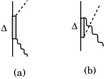
Figure 4: The $\Delta$ current contributions. Dashed lines represent pion. Waved lines represent either the vector field or axial vector field.

The $\Delta$ has two contributions to weak pion production reactions, as shown in Fig. 4. The resonant amplitude is due to the formation of a $\Delta$ in s-channel(Fig. 4a). The cross $\Delta$ term, Fig. 4b, is part of the non-resonant amplitude. Each term has a corresponding pion pole term illustrated in Fig. 3 and these pion pole terms must be also included in our investigations.

To calculate these $\Delta$ amplitudes, we need to define the matrix elements $<\Delta\mid V^{\mu}\mid N>$ and $<\Delta\mid A^{\mu}\mid N>$. The vector current matrix element $<\Delta\mid V^{\mu}\mid N>$ can be obtained from SL model by appropriate isospin rotations. Here we focus on the axial vector current matrix element.

It is well knownadler ; hhm that the most general form of axial vector current matrix element can be written as

$$<\Delta|A^{\mu i}|N>=\bar{u}_{\Delta\nu}({\bm{p}}^{\prime})\Gamma^{\mu\nu}_{A}T^{i}u({\bm{p}})$$ (76)

with

$$\Gamma^{\mu\nu}_{A} = d_{1}(q^{2})g^{\mu\nu}+\frac{d_{2}(q^{2})}{m_{N}^{2}}P_{\alpha}(q^{\alpha}g^{\mu\nu}-q^{\nu}g^{\alpha\mu})-\frac{d_{3}(q^{2})}{m_{N}^{2}}p^{\nu}q^{\mu}+i\frac{d_{4}(q^{2})}{m_{N}^{2}}\epsilon^{\mu\nu\alpha\beta}P_{\alpha}q_{\beta}\gamma_{5}]$$

where $u_{\Delta\nu}({\bm{p}})$ is the spin $3/2$ Rarita-Schwinger spinor, $q=p^{\prime}-p$, $P=p^{\prime}+p$, and $T^{i}$ is the $i-$th component of the isospin transition operator(defined by the reduced matrix element $<3/2\mid\mid{\bm{T}}\mid\mid 1/2>=-<1/2\mid\mid{\bm{T}}^{+}\mid\mid 3/2>=2$ in Edmonds conventionedmonds ).

It is useful to explore here the meaning of each form factor of Eq. (76). Since $u_{\Delta\nu}({\bm{p}}^{\prime})=u({\bm{p}}^{\prime})\epsilon_{\Delta,\nu}({\bm{p}}^{\prime})$, where $\epsilon_{\Delta,\nu}({\bm{p}}^{\prime})$ is an unit four vector, we can rewrite Eq. (76) as

$$<\Delta|A^{\mu i}|N> = \bar{u}({\bm{p}^{\prime}})[(d_{1}(q^{2})+\frac{P\cdot q}{m_{N}^{2}}d_{2}(q^{2}))\epsilon_{\Delta}^{\mu}+(-d_{2}(q^{2})P^{\mu}+d_{3}(q^{2})q^{\mu})\frac{q\cdot\epsilon_{\Delta}}{m_{N}^{2}}$$ (77)

$$+i\frac{d_{4}(q^{2})}{m_{N}^{2}}\epsilon^{\mu\nu\alpha\beta}\epsilon_{\Delta,\nu}P_{\alpha}q_{\beta}\gamma_{5}]T^{i}u({\bm{p}}).$$

In the rest frame of a $\Delta$ on the resonance energy( $p^{\prime}=(m_{\Delta},\bm{0}),p=(E_{N}(q),-\bm{q}),q=(m_{\Delta}-E_{N}(q),\bm{q}),\epsilon_{\Delta}=(0,\bm{\epsilon})$, $\bar{u}(p^{\prime}=(m_{\Delta},0))=(\chi^{+}_{\Delta},0)$, and $u(p)\propto\chi_{N}$, where $\chi_{\beta}$ is the Pauli spinor), the space and time components of Eq. (77) become

$$<\Delta|\bm{A}^{i}|N> = \sqrt{\frac{E_{N}+m_{N}}{2m_{N}}}[(d_{1}+\frac{m_{\Delta}^{2}-m_{N}^{2}}{m_{N}^{2}}d_{2})\bm{S}-(d_{2}+d_{3})\frac{(\bm{S}\cdot\bm{q})\bm{q}}{m_{N}^{2}}$$ (78)

$$-id_{4}\frac{\bm{S}\times\bm{q}(\bm{\sigma}\cdot\bm{q})}{m_{N}^{2}(E_{N}+m_{N})}]T^{i},$$

$$<\Delta|A^{0i}|N> = \sqrt{\frac{E_{N}+m_{N}}{2m_{N}}}[d_{2}\frac{\bm{S}\cdot\bm{q}(m_{\Delta}+E_{N})}{m_{N}^{2}}-d_{3}\frac{\bm{S}\cdot\bm{q}(m_{\Delta}-E_{N})}{m_{N}^{2}}]T^{i},$$ (79)

where we have defined the transition spin $\bm{S}=\chi^{+}_{\Delta}\bm{\epsilon}\chi_{N}$ (the reduced matrix element $<\frac{3}{2}\mid\mid{\bm{S}}\mid\mid\frac{1}{2}>$ is identical to that of the transition isospin $\bm{T}$). The above expression suggests that $d_{1},d_{2}$ terms describe the Gamow-Teller transition and $d_{4}$ describes the quadrupole transition. The term of $d_{3}$ comes from the pion pole term illustrated in Fig. 3.

For simplicity, we now follow Ref.hhm to fix the form factors $d_{i}(q^{2})$ at $q^{2}=0$ using the non-relativistic constituent quark model. The axial vector current operator for a constituent quark is derived from taking the non-relativistic limit of the standard form $g_{Aq}\bar{q}\gamma^{\mu}\gamma_{5}\frac{\tau}{2}q$. By using a procedure similar to Eq. (74) based on the PCAC relation, we then can extend the resulting current operator to also include the pion pole term contribution(Fig. 3) induced by the current $-F\partial^{\mu}\vec{\pi}$ of Eq. (60). The total axial vector current operators associated with a constituent quark model are found to be of the following forms

$$<\bm{p}^{\prime}\mid\bm{A}^{i}\mid\bm{p}> = g_{Aq}[\bm{\sigma}+\frac{\bm{q}}{q^{2}-m_{\pi}^{2}}\bm{\sigma}\cdot\bm{q}]\frac{\tau^{i}}{2},$$ (80)

$$<\bm{p}^{\prime}\mid A^{0\ i}\mid\bm{p}> = g_{Aq}[\frac{\bm{\sigma}\cdot(\bm{p}+\bm{p}^{\prime})}{2m_{q}}+\frac{q^{0}}{q^{2}-m_{\pi}^{2}}\bm{\sigma}\cdot\bm{q}]\frac{\tau^{i}}{2},$$ (81)

where $\bm{p}$ is the quark momentum, $\sigma$ and $\tau$ are the quark spin and isospin operators respectively. By using the standard non-relativistic s-wave quark wave functions for $N$ and $\Delta$, it is straightforward to obtain

$$<\bm{p}_{N}^{\prime}\mid\bm{A}^{i}\mid\bm{p}_{N}> = (\frac{5}{3}g_{Aq})[\bm{\sigma}+\frac{\bm{q}}{q^{2}-m^{2}_{\pi}}\bm{\sigma}\cdot\bm{q}]\frac{\tau^{i}}{2},$$ (82)

$$<\bm{p}_{N}^{\prime}\mid A^{0\ i}\mid\bm{p}_{N}> = (\frac{5}{3}g_{Aq})[\frac{\bm{\sigma}\cdot(\bm{p}_{N}^{\prime}+\bm{p}_{N})}{2(3m_{q})}+\frac{q^{0}}{q^{2}-m_{\pi}^{2}}\bm{\sigma}\cdot\bm{q}]\frac{\tau^{i}}{2},$$ (83)

and

$$<\bm{p}_{\Delta}\mid\bm{A}^{i}\mid\bm{p}_{N}> = \frac{1}{2}\sqrt{\frac{72}{25}}(\frac{5}{3}g_{Aq})[\bm{S}+\frac{\bm{q}}{q^{2}-m^{2}_{\pi}}\bm{S}\cdot\bm{q}]T^{i},$$ (84)

$$<\bm{p}_{\Delta}\mid A^{0\ i}\mid\bm{p}_{N}> = \frac{1}{2}\sqrt{\frac{72}{25}}(\frac{5}{3}g_{Aq})[\frac{\bm{S}\cdot(\bm{p}_{\Delta}+\bm{p}_{N})}{2(3m_{q})}+\frac{q^{0}}{q^{2}-m_{\pi}^{2}}\bm{S}\cdot\bm{q}]T^{i}.$$ (85)

In above equations, ${\bm{p}}_{N}$ and ${\bm{p}}_{\Delta}$ are the momenta for $N$ and $\Delta$ respectively, and we have expressed the right hand sides in terms of usual nucleon spin and isospin operators and the $\Delta$-$N$ transition operators $\bm{S}$ and $\bm{T}$(as defined above).

If we set $3m_{q}=m_{N}$ and $\frac{5}{3}g_{Aq}=g_{A}(0)=1.26$, Eqs. (82) and (83) can be identified with the usual non-relativistic form for the nucleon axial current matrix element at $q^{2}=0$. This then fixes the value of $g_{Aq}$ which also determine Eqs. (84)-(85) for the axial N-$\Delta$ transitions.

Comparing Eqs. (84)-(85) evaluated at the $\Delta$ rest frame($\bm{p}_{\Delta}=0$) and Eqs. (78)-(79) taken in the non-relativistic limit($E_{N}\rightarrow m_{N}$ and $q^{2}/m_{N}^{2}\rightarrow 0$), we find that

$$d_{1}(Q^{2}_{0}) = g^{*}_{A}(Q^{2}_{0})(1+\frac{m^{2}_{\Delta}-m^{2}_{N}}{2m_{N}(m_{\Delta}+m_{N})})$$ (86)

$$d_{2}(Q^{2}_{0}) = -g^{*}_{A}(Q^{2}_{0})\frac{m_{N}}{2(m_{\Delta}+m_{N})}$$ (87)

$$d_{3}(Q^{2}_{0}) = -g^{*}_{A}(Q^{2}_{0})\frac{m^{2}_{N}}{q^{2}-m_{\pi}^{2}}$$ (88)

where $g_{A}^{*}(Q^{2}_{0})=\frac{1}{\sqrt{2}}\frac{6}{5}g_{A}$. Here we also follow Ref.hhm to assume that the quark model results Eqs. (84)-(85) are for the momentum transfer $q_{0}=(m_{\Delta}-m_{N},\bm{0})$ and $Q^{2}_{0}=-q^{2}_{0}=(m_{\Delta}-m_{N})^{2}$. Eqs. (86)-(88) agree with the results of Ref.hhm if we neglect the difference between $m_{N}$ and $m_{\Delta}$.

To account for the $q^{2}$-dependence, we assume that

$$d_{i}(Q^{2})=d_{i}(0)F(Q^{2})$$ (89)

where $F(Q^{2})$ will be specified in the next section. For a given choice of $F(Q^{2})$, we can use Eqs. (86)-(88) to obtain $d_{i}(0)=d(Q^{2}_{0})/F(Q^{2}_{0})$. The form factors $d_{i}(Q^{2})$ for $i=1,2,3$ of the covariant form Eq.(76), which is used in our numerical calculations, are then completely fixed by the constituent quark model calculation. We neglect the $\Delta$ deformation in this work and set $d_{4}(q^{2})=0$.

With the axial N-$\Delta$ vertex specified above and the $\pi N$ model constructed in Ref.sl1 , the dressed $AN\rightarrow\Delta$ vertices (i.e. Eqs. (4)-(5)) can be calculated for evaluating the resonant amplitude Fig. 4a(i.e. the second term of Eq. (2)). With the $\pi N\Delta$ interaction Lagrangian $L_{\pi N\Delta}=f_{\pi N\Delta}/m_{\pi}\bar{\psi}^{\mu}_{\Delta}(x)\vec{T}N(x)\cdot\partial_{\mu}\vec{\pi}(x)$ of SL model, the cross $\Delta$ term (Fig. 4b) is found to be

$$A^{\mu}_{\Delta E}(k,j,q,i)=\frac{1}{(2\pi)^{3}}\sqrt{\frac{m_{N}^{2}}{2E_{\pi}(k)E_{N}(p)E_{N}(p^{\prime})}}\bar{u}({\bm{p}}^{\prime})I^{\mu}_{\Delta E}(k,j,q,i)u({\bm{p}}),$$ (90)

with

$$I^{\mu}_{\Delta E}(k,j,q,i)=i\frac{f_{\pi N\Delta}}{m_{\pi}}T^{+}_{i}\Gamma_{A}^{\dagger\mu\nu}S_{\nu\delta}(p-k)T_{j}k^{\delta}.$$ (91)

where the Rarita-Schwinger propagator $S_{\mu\nu}(p)$ given explicitly in Eq. (3.18) of Ref.sl1 .

The above derivations allow us to use the constituent quark model to calculate the $\Delta$ amplitudes. This completes our derivations of the weak current matrix elements which are the input to the dynamical equations Eqs. (2)-(4) with the sub-index $\gamma$ replaced by either $V$ or $A$.

IV Results and Discussions

As presented in subsection III.A, the non-$\Delta$ amplitudes, illustrated in Figs. 1-2, do not have any adjustable parameters in this investigation. While more theoretical investigations may be needed to refine these non-resonant amplitudes, it may not be necessary at this time since the weak pion production data are still limited. Instead, we focus on the investigation of the axial vector N-$\Delta$ transition form factors defined in subsection III.B.

To proceed, we first recall the N-$\Delta$ form factors introduced in SL model. For the bare magnetic M1 N-$\Delta$ transition, it was taken as

$$G_{M}(Q^{2})=G_{M}(0)R_{SL}(Q^{2})G_{D}(Q^{2}),$$ (92)

where $G_{D}(Q^{2})=1/(1+Q^{2}/M^{2}_{V})^{2}$ with $M^{2}_{V}=0.71$ GeV² is the usual dipole form factor of the nucleon, and the correction factor is defined as

$$R_{SL}=(1+aQ^{2})\exp(-bQ^{2}).$$ (93)

By fitting the pion photoproduction and electroproduction data up to $Q^{2}=4$ (GeV/c)², it was found that $G_{M}(0)=1.85$, $a=0.154$ (GeV/c)^-2 and $b=0.166$ (GeV/c)^-2. Here we remark that if we follow the same procedure given in section III.B to also calculate the $\gamma N\rightarrow\Delta$ transition using non-relativistic quark model, we find that the quark model yields $G^{Q.M.}_{M}(Q^{2}_{0})=2.37$ for $Q^{2}_{0}=(m_{\Delta}-m_{N})^{2}$. This value is very close to the value $G_{M}(Q^{2}_{0})=2.42$ which can be obtained from SL model by using Eqs. (92)-(93). This suggests that the use of Eqs. (86)-(88) for defining $d_{i}(Q^{2}_{0})$ of the axial N-$\Delta$ form factors is a good starting point of our investigations. As a continuation of SL model, we therefore first consider a model, called Model I, which assumes that the form factor of Eq. (89) is

$$F(Q^{2})=R_{SL}(Q^{2})G_{A}(Q^{2}),$$ (94)

where $R_{SL}(Q^{2})$ is given in Eq. (93), and $G_{A}(Q^{2})=1/(1+Q^{2}/M^{2}_{A})^{2}$ with $M_{A}=1.02$GeV of the nucleon axial form factormeissner .

We first compare the total cross sections predicted by Model I with the datadata79 . The results are shown in Fig. 5. We see that the predictions(solid curves) agree reasonably well with the data for three pion channels. For the data on neutron target, our predictions(solid curves in the middle and lower figures) are in general lower than the data. This is perhaps related to the procedures used in Ref.data79 to extract these data from the experiments on deuteron target.

One of the main features of the dynamical approach taken in this work is to renormalize(dress) the N-$\Delta$ transitions with the dynamical pion cloud effect, as described Eqs. (4)-(5). The importance of this effect is shown in Fig. 5. We see that our full calculations(solid curves) are reduced significantly to dotted curves if we turn off the dynamical pion cloud effects. If we further turn off the contributions from bare N-$\Delta$ transitions, we obtain the dashed curves which correspond to the contributions from the non-resonant amplitudes(Figs. 1-3). Clearly, the nonresonant amplitudes are weaker, but are also essential in getting the good agreement with the data since they can interfere with the resonant amplitudes.

We next compare the $Q^{2}$-dependence of the differential cross sections $d\sigma/dQ^{2}$ predicted by Model I with the data from ANLdata79 , BNLdata90 , and CERNdata89 . Here we need to account for the variation of neutrino flux in the experiments at ANLdata79 and BNLdata90 . We calculate the following quantity

$$\frac{d\bar{\sigma}}{dQ^{2}}=[\int_{E_{min}}^{E_{max}}dE_{\nu}\frac{N(E_{\nu})}{\sigma_{model}(E_{\nu})}\frac{d\sigma_{model}}{dQ^{2}}(E_{\nu})]/[\int_{E_{min}}^{E_{max}}dE_{\nu}\frac{N(E_{\nu})}{\sigma_{model}(E_{\nu})}]$$ (95)

where $N(E_{\nu})$ is the distribution of events in neutrino energy $E_{\nu}$ which is within the range between $E_{min}$ and $E_{max}$, and $\sigma_{model}(E_{\nu})$ is the calculated total cross section. The distributions $N(E_{\nu})$ are given in Fig. 6 of Ref.data79 and Fig. 4 of Ref.data90 .

The predictions from Model I are compared with the ANL datadata79 in Fig. 6. We see that our predictions(solid curve) agree reasonable well with the data both in magnitude and $Q^{2}-$dependence. In Fig. 6 we also compare the contributions from vector current(dot-dashed curve) and axial vector current(dotted curve). They have rather different $Q^{2}$-dependence in the low $Q^{2}$ region and interfere constructively with each other to yield the solid curve of the full results. Since vector current contributions are very much constrained by the $(e,e^{\prime}\pi)$ data, the results of Fig. 6 suggest that the axial vector currents constructed in section III are consistent with the data.

For comparing with the BNL datadata90 , we normalize the calculated $d\bar{\sigma}/dQ^{2}$ to the events data of Fig. 5 of Ref.data90 at $Q^{2}=0.2$ (GeV/c)². As shown in Fig. 7, the data can be reproduced very well by Model I. The BNL data was used in the most recent attemptdata90 to extract the axial N-$\Delta$ form factor. We will discuss this later.

The comparison with CERN datadata89 is given in Fig. 8. Here the data have some structure, which is perhaps mainly due to the poor statistics of experiment. We see that model I can reproduce the main feature of the $Q^{2}$-dependence.

To explore the effects due to the dynamical pion cloud on the N-$\Delta$ form factors, it is instructive to recall here the results of Ref.sl2 for the magnetic M1 $\gamma N\rightarrow\Delta$ transition. This result is displayed in the left panel of Fig. 9. We see that the pion cloud effect is essential in explaining the empirical values extracted directly from the data. The corresponding dynamical pion cloud effect on the axial N-$\Delta$ form factor is shown in the right panel of Fig. 9. We again see fairly sizable contribution from dynamical pion cloud. We stress that the empirical form factor, such as that extracteddata90 from BNL data, can only be compared with our dressed form factor, since the dressed form factor, not the bare form factor, directly determines the reaction amplitude Eq. (2). The differences between the solid and dotted curves in Fig. 9 explain the observationhhm that the quark model prediction of axial vector N-$\Delta$ strength at $Q^{2}\rightarrow 0$ is lower than the empirical value of Ref.data90 by about 35 $\%$. This is simply due to the fact that the dynamical pion cloud is not included in constituent quark model calculation and most of the hadron model calculations of N-$\Delta$ transitions. It is also interesting to observe from Fig. 9 that the pion cloud effect on the axial N-$\Delta$ form factor is mainly to increase the magnitude, not much to change the slope. On the other hand, both the magnitude and slope of the magnetic M1 form factor (left-hand side of Fig. 9) are significantly changed by including the pion cloud effects.

To see the dependence of our predictions on the parameterization of axial N-$\Delta$ form factor, we next consider Model II which differs from Model I only in replacing the correction factor $R_{SL}$ of Eq. (94) by a different form. Rather arbitrarily, we consider a form used in Refs.adler ; data90 ; hhm . The axial N-$\Delta$ form factor in this model II is also defined by Eq. (89) with

$$F(Q^{2})=R_{II}(Q^{2})G_{A}(Q^{2})$$ (96)

where $G_{A}(Q^{2})$ is the axial nucleon form factor of Eq. (94) and

$$R_{II}=(1+a\frac{Q^{2}}{b+Q^{2}})$$ (97)

with $a=-1.21$ and $b=2$ (GeV/c)².

The main difference between Model I and Model II is in determining $d_{i}(0)=d(Q^{2}_{0})/F(Q^{2}_{0})$ from the quark model values $d_{i}(Q^{2}_{0})$ given in Eqs. (86)-(88). We find that $1/F(Q^{2}_{0})=1.20$ for Model I and $1/F(Q^{2}_{0})=1.26$ for Model II. Thus these two models are already different at $Q^{2}\rightarrow 0$. Their $Q^{2}$-dependence are compared in Fig. 10. We see that the form factor of Model II(dotted curve) are much lower than that of Model I(solid curve). Consequently, the weak pion production cross sections calculated from Model II are found to be about 20 $\%$ lower than the data. This is illustrated in Fig. 11. We find that the model II can fit the data better if we increase the strengths $d_{i}(0)$ of axial N-$\Delta$ form factor by 20$\%$. The results shown in Figs. 10 and 11 demonstrate the sensitive of the data to the form of the bare axial N-$\Delta$ form factor. The data clearly favor the form factor Eq. (94).

As seen in Eqs. (2) and (4), the empirical N-$\Delta$ form factor extracted directly from the data, such as those obtained in Ref.data90 can only be compared with our dressed form factor $\bar{\Gamma}$. The comparison is given in Fig. 12. We see that they do not agree well, in particular in the high $Q^{2}$ region. The differences mainly come from the fact that the non-resonant amplitudes of the Adler Model, which was useddata90 in extracting the empirical N-$\Delta$ form factors, are rather different from what we have in our dynamical model. With the very limited data, it is not possible to exclude one of these two rather different results. Clearly, more precise data are needed for a better test of our models.

To stimulate future experimental efforts, we now present two predictions of Model I in Figs. 13 and 14. In Fig. 13, we present the $Q^{2}$-dependence of differential cross sections at $W=1.1,1.2,1.236,1.3$ GeV. The $W-$dependence at $Q^{2}=0.1,0.5,1.0,1.5$ (GeV/c)² is shown in Fig. 14.

V Conclusions

We have extended the dynamical model of Refs.sl1 ; sl2 to investigate weak pion production reactions in the $\Delta$ region. The calculations for neutrino-induced reactions have been performed by using the current matrix elements illustrated in Figs. 1-3. The parameters for the non-resonant terms(Figs. 1-2) are taken from the previous investigations of pion electroproduction. The bare N-$\Delta$ transitions at $Q^{2}\rightarrow 0$ are fixed by the constituent quark model. With the axial N-$\Delta$ form factor given in Eqs. (86)-(88), the predicted total cross sections and the differential cross sections $d\sigma/dQ^{2}$ agree reasonably well with the existing data.

We have analyzed the calculated N-$\Delta$ form factors. Similar to the finding of the $(e,e^{\prime}\pi)$ studiessl1 ; sl2 , we show that the constituent quark model prediction of axial vector N-$\Delta$ form factor at $Q^{2}\rightarrow 0$ is consistent with the data. The discrepancy observed in Ref.hhm is due to the dynamical pion cloud effect which is not included in the constituent quark model calculation.

An unsatisfactory aspect of the present investigation is the lack of extensive and good quality data. Thus the axial vector N-$\Delta$ from factor extracteddata90 from the data relied heavily on model assumptions and hence the origins of the differences seen in Fig. 12 are not clear. It will be very useful to have sufficient data for performing partial wave decomposition, like what have been routinely performed in $(e,e^{\prime}\pi)$ studies, such that the N-$\Delta$ form factor can be extracted model independently. Hopefully, the situation will be improved in the near future when new neutrino facilities will become available.

Figure 1: Non-$\Delta$ vector current contributions. Dashed lines represent pion. Waved lines represent the vector field.

Figure 2: Non-$\Delta$ axial vector current contributions. Dashed lines represent pion. Waved lines represent axial vector field.

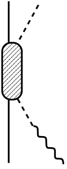
Figure 3: Pion-pole term of axial vector current contributions. The dashed-box represents the either the non-$\Delta$ mechanisms of Fig.2 or the crossed $\Delta$ mechanism of Fig.4(b).

Figure 5: Total cross sections of $N(\nu_{\mu},\mu^{-}\pi)N$ reactions predicted by Model I. The data are from Ref.data79 . The solid curves are from full calculations. The dotted curves are from turing off pion cloud effects on N-$\Delta$ transitions. The dashed curves are the contributions from the non-resonant amplitude.

Figure 6: Differential cross sections $d\bar{\sigma}/dQ^{2}$ of $p(\nu_{\mu},\mu^{-}\pi^{+})p$ reaction averaged over neutrino energies 0.5 GeV $<E_{\nu}<$ 6 GeV. The curves are from calculations using Eq. (95). The dotted curve(dot-dashed curve) is the contribution from axial vector current A (vector curent V). The solid curve is from our full calculations with V-A current. The data are from Ref.data79 .

Figure 7: The differential cross sections $d\bar{\sigma}/dQ^{2}$ of $p(\nu_{\mu},\mu^{-},\pi^{+})$ reaction calculated using Eq. (95). The data are from Ref.data90 .

Figure 8: Differential cross sections $d\sigma/dQ^{2}$ of $p(\nu_{\mu},\mu^{-}\pi^{+})p$ reaction at neutrino energy $E_{\nu}=$ 15 GeV. The data are from Ref.data89

Figure 9: The N-$\Delta$ form factors predicted by Model I: left panel: Magnetic M1 form factors given in Ref.sl2 , right panel: axial vector form factor. The solid curves are from full calculations. The dotted curves are obtained from turing off the pion cloud effects. $G_{D}=1/(1+Q^{2}/M^{2}_{V})^{2}$ with $M_{V}=0.84$ GeV is the usual proton form factor and $G_{A}=1/(1+Q^{2}/M^{2}_{A})^{2}$ with $M_{A}=1.02$ GeV is the axial nucleon form factor of Ref. meissner .

Figure 10: Bare axial N-$\Delta$ form factors for Model I(soild curve) and Model II(dotted curve).

Figure 11: The total cross sections of $p(\nu_{\mu},\mu^{-}\pi^{+})p$ calculated from Model I(soild curves) and Model II(dot curves).

Figure 12: Compare the dressed axial N-$\Delta$ form factor predicted by Model I(solid curve) with the empirical form factor(dot-dash curve) determined in Ref.data90 .

Figure 13: The predicted differential cross sections $d\sigma/dWdQ^{2}$ for $p(\nu_{\mu},\mu^{-}\pi^{+})p$ at neutrino energy $E_{\nu}=2$ GeV and invariant mass W=1.1(dashed), 1.2(dotted), 1.236(solid), 1.3(dot-dashed) GeV.

Figure 14: The predicted differential cross sections $d\sigma/dWdQ^{2}$ for $p(\nu_{\mu},\mu^{-}\pi^{+})p$ at neutrino energy $E_{\nu}=2$ GeV and $Q^{2}=$0.1(solid), 0.5(dashed), 1.0(dotted), 1.5(dot-dashed) (GeV/c)².