Neutrino emission in neutron stars

Abstract

Neutrino emissivities in a neutron star are computed for the neutrino bremsstrahlung process. In the first part the electro-weak nucleon-nucleon bremsstrahlung is calculated in free space in terms of a on-shell $T$-matrix using a generalized Low energy theorem. In the second part the emissivities are calculated in terms of the hadronic polarization at the two-loop level. Various medium effects, such as finite particle width, Pauli blocking in the $T$-matrix are considered. Compared to the pioneering work of Friman and Maxwell in terms of (anti-symmetrized) one-pion exchange the resulting emissivity is about a factor 4 smaller at saturation density.

I Introduction

The cooling of neutron stars proceeds via the weak interaction. Since in general one-body processes are kinematically forbidden the dominant reactions are assumed to be the neutral current two-particle processes

$$n+n\to n+n+\nu_{f}+\bar{\nu}_{f},$$ (1)

$$n+p\to n+p+\nu_{f}+\bar{\nu}_{f},$$ (2)

and the charged current “modified URCA” process

$$N+n\to N+p+\bar{\nu}_{e}+e^{-}.$$ (3)

Standard cooling scenarios are mostly based upon the pioneering work of Friman and Maxwell FM1979 . In essence their approach amounts to a convolution of the soft free space neutrino pair emission and two-body (modified) URCA processes (1-3) with a finite temperature free Fermi-gas model using Fermi’s golden rule to obtain the emission rate. In doing so a number of simplifying assumptions were made; in particular (i) the two-body interaction between the nucleons was approximated by a central Landau interaction plus a one-pion exchange to represent the tensor force, (ii) and only the non-relativistic limit was considered, (iii) since it is based upon the quasi-particle approximation non-perturbative effects such as the LPM effect were not taken into account, (iv) other medium effects such as Pauli blocking in the strong interaction were neglected. It is the aim of the present paper to investigate and possibly improve these assumptions.
In the first part we consider the reactions (1-2) in free space. Using the fact that the energy release in the bremsstrahlung process is very small we apply the soft bremsstrahlung formalism of Hanhart et al. HPR2000 and Timmermans et al. TKDD2002 . This allows one to express the bremsstrahlung process in the soft limit model independently in terms of an on-shell $T$-matrix, i.e. phase shifts. In this way we are able to judge the accuracy of past bremsstrahlung calculations, which were mostly based upon the use of a one pion exchange (OPE) approximation in the non-relativistic limit FM1979 ; VS1986 . In the latter case simplifications occur such as the vanishing of the vector current matrix elements.
In the second part we consider the process (1) in the medium. To describe the cooling process of neutron stars through neutrino emission the application of Fermi’s golden rule in the quasi particle approximation (QPA) was mostly used in the past. To compute emissivities beyond QPA one needs to start from quantum transport equations. The essential physics is then contained in the neutrino self-energies, which appear in the loss and gain terms. We will compare the diagrams at the hadron two loop level. It appears that only in lowest order in the imaginary part of the hadronic self-energies the use of closed diagrams and the application of Fermi’s golden rule coincide.
From the generalized Low-energy theorem TKDD2002 ; HPR2000 it follows that the use of the QPA leads to a infrared divergent amplitude, $1/\omega.$ The latter is predicted to be quenched KV in a medium whenever the mean free path of the nucleons becomes on the order of the formation length of the lepton pair. This is also known as the Landau-Pomeranchuk-Migdal(LPM) effect in case of electromagnetic interactions). The importance of this effect we study by including a finite single particle width (imaginary part of the self-energy) which depends on energy and temperature.
In practice in calculating the collision integral one needs to specify the appropriate diagrams and make assumptions about hadronic interactions. In doing so one must be careful that symmetries like gauge invariance of the vector current are not violated. We also estimate the Pauli blocking by replacing the $T$-matrix by a in-medium $G$-matrix. In Sedrakian and Dieperink SD2000 the neutrino emissivity was computed including the LPM effect, however in the OPE approximation
Many properties of superfluid matter such as pairing are still known with large uncertainty. Therefore only non-superfluid matter will be considered. For recent papers about pairing we refer to Gusakov G2002 and Yakovlev et al. YKH2002 .
Although we will apply the present formalism to neutrino pair emission in neutral weak current processes, it is equally valid for soft electromagnetic bremsstrahlung.
This paper is organized as follows. In section 2 we discuss electroweak bremsstrahlung in free space; in section 3 the in-medium process is discussed at the two-loop level. In section 4 results are presented showing the effects of various approximations. In the appendix a summary of quantum transport theory and finite temperature Green functions is presented.

II Electroweak bremsstrahlung in free space

Figure 1: Diagrams for neutrino pair bremsstrahlung of order $1/\omega$ with radiation from external legs.

II.1 Soft electroweak bremsstrahlung amplitude

The $\nu\overline{\nu}$ pair emission in a neutron star is characterized by a very small energy transfer (on the order of the temperature $T\simeq 1$ MeV), much smaller than any other scale in the process like $m_{\pi}$ or $p_{F}$. Therefore it is natural to consider the $NN\rightarrow NN\nu\overline{\nu}$ process in the ultra-soft limit. For simplicity and also to be consistent with the low density limit of the medium we will first consider this process in free space.
Here the treatment of soft $NN$ electroweak bremsstrahlung, discussed in more detail in Ref. TKDD2002 , is summarized. Analogously to the electromagnetic bremsstrahlung (Low, Low ), the first two terms of the expansion in powers of the energy-momentum transfer $|\vec{q}|<\omega$ of the electroweak bremsstrahlungs amplitude are determined by the amplitude for the corresponding non-radiative process $M=A/\omega+B+O(\omega).$ In the ultra-soft regime ($\omega/p<<1$, where $p$ is the nucleon momentum) the $B$ and higher order terms can be neglected. The amplitude of the diagrams in Fig. 1 with radiation from external legs only is given by HPR2000 ,TKDD2002

$$M_{\nu}^{ext,a}=T_{1}{S(p_{1}-q)}{\Gamma^{a}_{\nu}}+{{\Gamma^{a}_{\nu}}}{{S(p^{\prime}_{1}+q)}}T^{\prime}_{1}+\{1\leftrightarrow 2\}.$$ (4)

The $A$ term in the Low expansion is obtained by considering the limit $|\vec{q}|<\omega\rightarrow 0$ of $\omega M_{\nu}^{ext,a}$; to this end we expand the various $T$’s with one nucleon off its mass shell,

$$T_{1}=<p^{\prime}_{1},p^{\prime}_{2}|T|p_{1}-q,p_{2}>, T^{\prime}_{1}=<p^{\prime}_{1}+q,p^{\prime}_{2}|T|p_{1},p_{2}>,$$ (5)

around the on-shell point $T_{0}$,

$$T_{1}=T_{0}-q.\frac{\partial}{\partial p_{1}}T_{0}+...,\ T^{\prime}_{1}=T_{0}+q.\frac{\partial}{\partial p^{\prime}_{1}}T_{0}+...\ ,$$ (6)

and the nucleon propagator $S$ as

$$S(p\pm q)=\frac{\Lambda^{+}(p)+\Lambda^{-}(p)}{\!\not\!{p}\pm\!\not\!{q}-m}\approx\pm\frac{2m\Lambda^{+}(p)}{2p.q}+O(1)$$ (7)

with $\Lambda^{\pm}(p)=\frac{\pm\!\not\!{p}+m}{2m}$.

The hadronic weak interaction vertex in the limit $q\rightarrow 0$ is given by

$$\Gamma^{a}_{\nu}=\frac{G_{F}}{\sqrt{2}}\gamma_{\nu}(c_{V}-c_{A}\gamma_{5})\frac{\tau_{a}}{2},$$ (8)

where $G_{F}$ is the Fermi weak coupling constant and $\tau$ is the isospin-operator. The vector and axial-vector coupling constants $c_{V}$ and $c_{A}$ are for neutrons $c^{n}_{V}=-1$;  $c^{n}_{A}=-g_{A}=-1.26$ and for protons $c^{p}_{V}=1-4\sin^{2}\Theta_{W}\approx 0.08$;  $c^{p}_{A}=g_{A}=1.26$.
Since the initial/final particles are on mass-shell one has the relations $(\!\not\!{p}+m)\gamma_{\nu}u(p)=2p_{\nu}u(p)$ and $\overline{u}(p)\gamma_{\nu}(\!\not\!{p}+m)=2p_{\nu}\overline{u}(p)$, which are useful for the vector current. As a result in the ultra-soft region ($q/p<<1$) the vector and axial-vector current matrix element are given by

$$M^{V,a}_{\nu}=\frac{G_{F}c_{V}}{2\sqrt{2}}\Bigg{(}-T_{0}\frac{p_{1\nu}}{p_{1}.q}\tau^{a}+\tau^{a}\frac{p^{\prime}_{1\nu}}{p^{\prime}_{1}.q}T_{0}\Bigg{)}+\{1\leftrightarrow 2\}$$ (9)

and

$$M^{A,a}_{\nu}=\frac{2mG_{F}c_{A}}{2\sqrt{2}}\Bigg{(}-T_{0}\frac{\Lambda^{+}(p_{1})}{2p_{1}.q}\gamma_{\nu}\gamma_{5}\tau^{a}+\gamma_{\nu}\gamma_{5}\tau^{a}\frac{\Lambda^{+}(p^{\prime}_{1})}{2p^{\prime}_{1}.q}T_{0}\Bigg{)}+\{1\leftrightarrow 2\},$$ (10)

respectively. Naturally the vector current is conserved: $q^{\nu}M^{V,a}_{\nu}=0$.

II.2 Structure of the elastic $NN$ scattering amplitude

It is clear that the amplitudes in Eqs. (9) and (10) depend on the Lorentz structure of $T_{0}$. For the elastic $NN$ scattering amplitude GGMW1960 ; TW1985 for the process $N(p_{1})+N(p_{2})\rightarrow N(p^{\prime}_{1})+N(p^{\prime}_{2})$, the covariant form of the on-shell $T$-matrix can be expressed as

$$T=T^{dir}+T^{exch}=\sum_{I=0,1}\sum_{\alpha=1}^{5}F^{(I)}_{\alpha}(s,t,u)\Big{[}\overline{u}(p^{\prime}_{2})\Omega_{\alpha}u(p_{2})\overline{u}(p^{\prime}_{1})\Omega^{\alpha}u(p_{1})$$

$$+(-)^{\alpha}\overline{u}(p^{\prime}_{1})\Omega_{\alpha}u(p_{2})\overline{u}(p^{\prime}_{2})\Omega^{\alpha}u(p_{1})\Big{]}B_{I},$$ (11)

where the five Fermi covariants are

$$\Omega_{\alpha}=(\Omega_{1},\Omega_{2},\Omega_{3},\Omega_{4},\Omega_{5})=(1,\sigma_{\mu\nu}/\sqrt{2},\gamma_{5}\gamma_{\nu},\gamma_{\nu},\gamma_{5}).$$ (12)

The projection operators on iso-singlet and iso-triplet states are

$$B_{0}=(1-\vec{\tau}_{1}.\vec{\tau}_{2})/4,\ \ B_{1}=(3+\vec{\tau}_{1}.\vec{\tau}_{2})/4,$$ (13)

respectively. $F^{(I)}_{\alpha}(s,t,u)$ are the invariant functions of the Mandelstam variables $s=-(p_{1}+p_{2})^{2}$, $t=-(p^{\prime}_{1}-p_{1})^{2}$, and $u=-(p^{\prime}_{2}-p_{1})^{2}$. For the $nn\nu\overline{\nu}$ and $np\nu\overline{\nu}$ process the isospin combinations needed are

$$F^{(nn)}_{\alpha}(s,t,u)=F^{(pp)}_{\alpha}(s,t,u)=F^{(1)}_{\alpha}(s,t,u)$$

$$F^{(np)}_{\alpha}=(F^{(1)}_{\alpha}(s,t,u)+F^{(0)}_{\alpha}(s,t,u))/2$$ (14)

for $\alpha=1,...,5$. For later use, it is convenient to put the spinors in the exchange term in the “normal order” by introducing the functions

$$T^{(I)}_{\alpha}(s,t,u)=F^{(I)}_{\alpha}(s,t,u)+\sum_{\beta=1}^{5}(-1)^{\beta}C_{\alpha\beta}F^{I}_{\beta}(s,t,u),$$ (15)

where $C_{\alpha\beta}$ are elements of the Fierz transformation, the explicit form is given GGMW1960 ; TW1985 . Then Eq. (11) can be rewritten as

$$T=\sum_{I=0,1}\sum_{\alpha=1}^{5}T^{(I)}_{\alpha}(s,t,u)\overline{u}(p^{\prime}_{2})\Omega_{\alpha}u(p_{2})\overline{u}(p^{\prime}_{1})\Omega^{\alpha}u(p_{1})B_{I}.$$ (16)

Since for a comparison we will need the cross section in the non-relativistic limit, we also give the required non-relativistic decomposition of $T$ (we will reserve latin indices for the non-relativistic $T$-matrix)

$$T=\sum_{v=1}^{5}{\cal T}_{v}(s,t,u)O_{v},$$ (17)

where

$${\cal T}_{v}\equiv({\cal T}_{1},{\cal T}_{2},{\cal T}_{3},{\cal T}_{4},{\cal T}_{5})\equiv(T_{C},T_{Q},T_{T1},T_{T2},T_{SO})$$ (18)

and the five independent two-body operators

$$O_{v} \equiv (1,\vec{\sigma}_{1}\cdot\vec{n}\ \vec{\sigma}_{2}\cdot\vec{n},\vec{\sigma}_{1}\cdot\vec{k}\ \vec{\sigma}_{2}\cdot\vec{k},\vec{\sigma}_{1}\cdot\vec{k}^{\prime}\ \vec{\sigma}_{2}\cdot\vec{k}^{\prime},\vec{\sigma}_{1}\cdot\vec{n}+\vec{\sigma}_{2}\cdot\vec{n})$$ (19)

with $\hat{k}=(\vec{p}^{\prime}_{1}-\vec{p}_{1})/|\vec{p}^{\prime}_{1}-\vec{p}_{1}|$, $\hat{k^{\prime}}=(\vec{p}^{\prime}_{1}+\vec{p}_{1})/|\vec{p}^{\prime}_{1}+\vec{p}_{1}|$ and $\hat{n}=(\vec{k}^{\prime}\times\vec{k})/|\vec{k}^{\prime}\times\vec{k}|$ in the c.m.-system. The terms $T_{C}$,$T_{Q}$, $T_{T1}$ and $T_{SO}$ corresponds to the central, quadratic spin orbit, tensor and spin-orbit force, respectively; further we have a second tensor $T_{T2}$ (instead of the spin-spin force).

II.3 The $nn\nu\overline{\nu}$ process

We first treat the $n+n\rightarrow n+n+\nu+\overline{\nu}$ process. The vector current amplitude follows from Eq. (9)

$$M^{V}_{\nu} = \frac{G_{F}c^{n}_{V}}{2\sqrt{2}}\Big{(}-\frac{p_{1\nu}}{p_{1}.q}+\frac{p^{\prime}_{1\nu}}{p^{\prime}_{1}.q}-\frac{p_{2\nu}}{p_{2}.q}+\frac{p^{\prime}_{2\nu}}{p^{\prime}_{2}.q}\Big{)}$$ (20)

$$\sum_{\alpha=1}^{5}F^{(nn)}_{\alpha}\Big{[}\overline{u}(p^{\prime}_{2})\Omega_{\alpha}u(p_{2})\overline{u}(p^{\prime}_{1})\Omega^{\alpha}u(p_{1})+(-)^{\alpha}\{p^{\prime}_{2}\leftrightarrow p^{\prime}_{1}\}\Big{]}.$$

The axial-vector current amplitude follows from Eq. (10)

$$M^{A}_{\nu} = \frac{2mG_{F}g_{A}}{2\sqrt{2}}\sum_{\alpha=1}^{5}F^{(nn)}_{\alpha}\Big{[}\overline{u}(p^{\prime}_{2})\Omega_{\alpha}u(p_{2})\overline{u}(p^{\prime}_{1})\Big{(}-\Omega_{\alpha}\frac{\Lambda^{+}(p_{1})}{2p_{1}.q}\gamma_{\nu}\gamma_{5}$$ (21)

$$+\gamma_{\nu}\gamma_{5}\frac{\Lambda^{+}(p_{1})}{2p^{\prime}_{1}.q}\Omega^{\alpha}\Big{)}u(p_{1})+(-)^{\alpha}\overline{u}(p^{\prime}_{1})\Omega_{\alpha}u(p_{2})$$

$$\overline{u}(p^{\prime}_{2})\Big{(}-\Omega_{\alpha}\frac{\Lambda^{+}(p_{1})}{2p_{1}.q}\gamma_{\nu}\gamma_{5}+\gamma_{\nu}\gamma_{5}\frac{\Lambda^{+}(p^{\prime}_{2})}{2p^{\prime}_{2}.q}\Omega^{\alpha}\Big{)}u(p_{1})\Big{]}$$

$$+(1\leftrightarrow 2).$$

For later use we also give the non-relativistic limit and the first relativistic correction for the $nn\nu\overline{\nu}$ process by expanding the propagator in terms of $p/m$

$$\frac{1}{p.q}=\frac{1}{m\omega}\Bigg{(}1+\frac{\vec{p}.\vec{q}}{m\omega}+O\Big{(}\frac{p^{2}}{m^{2}}\Big{)}\Bigg{)}.$$ (22)

Application to the vector current amplitude yields

$$M^{V}_{\nu}=M^{V,NR}_{\nu}+\Delta M^{V}_{\nu}+O(p^{3}/m^{3}),$$ (23)

where the non-relativistic amplitudes $M^{V,NR}_{\nu}$ vanish and the leading corrections are given by

$$\Delta\vec{M}^{V}=\frac{G_{F}c^{n}_{V}}{2\sqrt{2}\omega^{2}m^{2}}\Bigg{(}\vec{p_{1}}\Big{(}\vec{p_{1}}\cdot\vec{q}\Big{)}-\vec{p}^{\prime}_{1}\Big{(}\vec{p}^{\prime}_{1}\cdot\vec{q}\Big{)}+\{1\leftrightarrow 2\}\Bigg{)}T^{nn}$$ (24)

$$\Delta M^{V}_{0}=\frac{\vec{q}\cdot\vec{\Delta M}^{V}}{\omega}$$ (25)

with $T^{nn}$ the non-relativistic reduction of the $I=1$ part of the $T$-matrix in Eq.(11). The vanishing of the non-relativistic vector amplitude generalizes the result of Friman and Maxwell FM1979 , where this cancellation was observed for Landau-type interaction and OPE, to the complete $nn$ $T$-matrix. This result is in fact, analogous to the absence of electric-dipole radiation in photon bremsstrahlung processes when the center-of-mass coincides with the center-of-charge of the radiating system, e.g. in $pp$ bremsstrahlung.
For the axial-current amplitude one obtains

$$M^{A}_{\nu}=M^{A,NR}_{\nu}+\Delta M^{A}_{\nu}+O(p^{2}/m^{2}),$$ (26)

where the non-relativistic amplitudes are given by

$$\vec{M}^{A,NR}=\frac{G_{F}g_{A}}{2\sqrt{2}\omega}[T^{nn},\vec{S}];\ \ M^{A,NR}_{0}=0,$$ (27)

and the leading relativistic corrections are

$$\Delta\vec{M}^{A}=\frac{G_{F}g_{A}}{2\sqrt{2}m\omega^{2}}\Bigg{(}T^{nn}\vec{\sigma}_{1}(\vec{p}_{1}\cdot\vec{q})-\vec{\sigma}_{1}T^{nn}(\vec{p}^{\prime}_{1}\cdot\vec{q})+\{1\leftrightarrow 2\}\Bigg{)}$$ (28)

$$\Delta M^{A}_{0}=\frac{G_{F}g_{A}}{2\sqrt{2}m\omega}\Bigg{(}T^{nn}(\vec{\sigma}_{1}\cdot\vec{p}_{1})-(\vec{\sigma}_{1}\cdot\vec{p}^{\prime}_{1})T^{nn}+\{1\leftrightarrow 2\}\Bigg{)}$$ (29)

with $\vec{S}=\vec{s}_{1}+\vec{s}_{2}$ the total spin of the $nn$ system. Eq. (27) has also been derived by Hanhart et al.HPR2000 , and Timmermans et al.TKDD2002 . One sees from Eq. (27) that in the non-relativistic limit there is no contribution from the central interaction $T_{C}$, but the axial-vector current amplitude receives contributions from all other terms.
The $pp\nu\overline{\nu}$ process can be treated analogously to $nn\nu\overline{\nu}$ process. The only differences are the coupling strength to the neutral weak current and the Coulomb corrections in the coefficients $F^{(1)}_{\alpha}$ of the $T$-matrix.

II.4 The $np\nu\overline{\nu}$ process

In the $n+p\rightarrow n+p+\nu+\overline{\nu}$ process the momenta will be denoted by $n$ and $n^{\prime}$ ($p$ and $p^{\prime}$), for the neutron (proton) in the initial and final state, respectively. In the ultra-soft region ($\omega/p<<1$) the vector current amplitude follows from Eq. (9)

$$M^{V}_{\nu} = \frac{G_{F}}{2\sqrt{2}}\Bigg{[}c^{n}_{V}\Big{(}-\frac{n_{\nu}}{n.q}+\frac{n^{\prime}_{\nu}}{n^{\prime}.q}\Big{)}+c^{p}_{V}\Big{(}-\frac{p_{\nu}}{p.q}+\frac{p^{\prime}_{\nu}}{p^{\prime}.q}\Big{)}\Bigg{]}$$ (30)

$$\sum_{\alpha=1}^{5}F^{(np)}_{\alpha}\Big{[}\overline{u}(p^{\prime})\Omega_{\alpha}u(p)\overline{u}(n^{\prime})\Omega^{\alpha}u(n)+$$

$$(-)^{\alpha}\{p^{\prime}\leftrightarrow n^{\prime}\}\Big{]}$$

and the axial-vector current amplitude from Eq. (10)

$$M^{A}_{\nu} = M^{A,dir}_{\nu}+M^{A,exch}_{\nu}$$ (31)

$$= -\frac{2mG_{F}g_{A}}{2\sqrt{2}}\Bigg{[}\sum_{\alpha=1}^{5}F^{(np)}_{\alpha}\bigg{[}\overline{u}(p^{\prime})\Omega_{\alpha}u(p)\overline{u}(n^{\prime})\Big{(}\Omega_{\alpha}\frac{\Lambda^{+}(n)}{2n.q}\gamma_{\nu}\gamma_{5}$$

$$-\gamma_{\nu}\gamma_{5}\frac{\Lambda^{+}(n^{\prime})}{2n^{\prime}.q}\Omega^{\alpha}\Big{)}u(n)-\Big{\{}(n,n^{\prime})\leftrightarrow(p,p^{\prime})\Big{\}}\bigg{]}$$

$$+(-)^{\alpha}\bigg{[}\overline{u}(n^{\prime})\Omega_{\alpha}u(p)\overline{u}(p^{\prime})\Big{(}\Omega_{\alpha}\frac{\Lambda^{+}(n)}{2n.q}\gamma_{\nu}\gamma_{5}$$

$$+\gamma_{\nu}\gamma_{5}\frac{\Lambda^{+}(p^{\prime})}{2p^{\prime}.q}\Omega^{\alpha}\Big{)}u(n)-\Big{\{}(n,n^{\prime})\leftrightarrow(p,p^{\prime})\Big{\}}\bigg{]}\Bigg{]}.$$

The exchange terms of axial-vector current matrix element are included explicitly in Eq. (31). The direct part is analogous to the expression in Eq. (21) for the $nn\nu\overline{\nu}$ process. The only difference is the appearance of a minus sign in the term, where the neutron en proton momenta are interchanged. This is a consequence of the sign difference of the axial-vector coupling constants for neutrons and protons.

The different structure of the exchange part (as compared to the $nn\nu\overline{\nu}$ process) comes from the sign difference between $c^{(p)}_{A}$ and $c^{(n)}_{A}$.
The expressions (30) and (31) simplify considerably, if one takes the non-relativistic limit. Using Eq. (22) one obtains for the vector current amplitude from Eq. (30)

$$\vec{M}^{V}=-\frac{G_{F}}{\sqrt{2}}\frac{c^{n}_{V}-c^{p}_{V}}{2\omega}\frac{\vec{k}}{m}T^{np},\ M^{V}_{0}=\frac{\vec{q}}{\omega}.\vec{M}^{V}$$ (32)

and for the axial-vector amplitude from Eq. (31)

$$\vec{M}^{A}=\frac{G_{F}g_{A}}{2\sqrt{2}\omega}\Big{(}[T^{np,dir},\vec{D}]+P_{\sigma}\{T^{np,exch},\vec{D}\}\Big{)},\ M^{A}_{0}=0,$$ (33)

where $\vec{k}=\vec{n}^{\prime}-\vec{n}=\vec{p}-\vec{p}^{\prime}$, $\vec{D}=(\vec{\sigma}_{1}-\vec{\sigma}_{2})$, the spin exchange operator is $P_{\sigma}=(1+\vec{\sigma_{1}}\cdot\vec{\sigma_{2}})/2$, $\{..,..\}$ denotes the anticommutator, $T^{np,dir}$ and $T^{np,exch}$ are given by the non-relativistic reduction of the direct and exchange parts of the $np$ $T$-matrix.
Note that in order $k/m\approx p/m$ in the $np$ case there is a non-vanishing contribution for the vector current amplitude. This is analogous to the case of photon bremsstrahlung in $NN$ scattering, where electric-dipole radiation is dominant for the $np$ case. The commutator in Eq. (33) receives contributions from tensor $T_{T1}$ and $T_{T2}$, quadratic spin-orbit $T_{Q}$ and spin-orbit $T_{SO}$ components of the direct part of the np $T$-matrix. The anticommutator receives in addition to $T_{T1}$, $T_{T2}$,$T_{Q}$ and $T_{SO}$ contributions from the exchange part of the np $T$-matrix also a central $T_{C}$ contribution.

II.5 Comparison with one boson exchange(OBE)

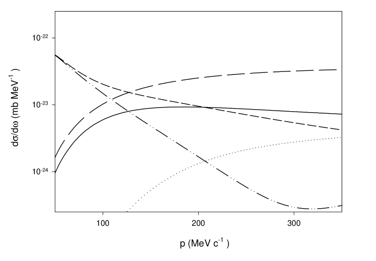
Figure 2: Cross section $d\sigma/d\omega$ for $n+n\rightarrow n+n+\nu+\overline{\nu}$ as a function of neutron momentum in the c.m. system, for $\omega=1$ MeV, and summed over neutrino flavors. Shown are the result for the OPE(long-dashed) and the full $T$-matrix (full curve); in addition the separate contributions of the $T$-matrix $T_{T1}+T_{T2}$ (short-dashed curve),$T_{SO}$ (dotted curve) and $T_{Q}$ (dashed double-dotted curve) are shown.

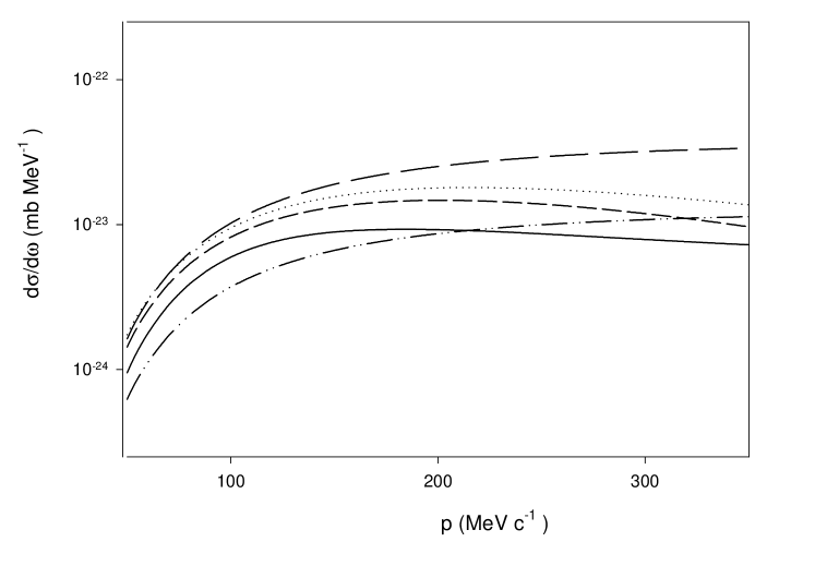
Figure 3: Cross section $d\sigma/d\omega$ for $n+n\rightarrow n+n+\nu+\overline{\nu}$ as a function of neutron momentum in the c.m. system, for $\omega=1$ MeV, and summed over neutrino flavors. Shown are the result for the OPE(long-dashed), OPtRE (short-dashed curve),OPRSE(dotted curve), OPE without the ”exchange” contribution (dashed double-dotted curve) and the full $T$-matrix (full curve).

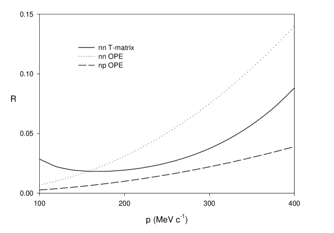
Figure 4: $R=\frac{|\sigma_{NR}-\sigma_{R}|}{\sigma_{NR}}$ with $\sigma_{NR}$ the non-relativistc cross section and $\sigma_{R}$ the cross section, in which also the first order relativistic corrections are included. Taking the OPE as the $NN$ interaction the $nn$ and $np$ bremsstrahlung ratios R are given by the dotted curve and the dashed curve, respectively. Also the $nn$ bremsstrahlung ratio R is shown using the $T$-matrix for the $NN$ interaction.

In this section we will calculate the neutrino emission cross section in free space. The expression for the cross section in the c.m. system is

$$\frac{d\sigma}{d\omega}=\frac{N_{f}}{4}\frac{m^{3}\sqrt{p^{2}-\omega E+\omega^{2}/4}}{6(2\pi)^{7}(E-\omega/2)p}\int d\Omega_{\tilde{p}}d^{3}q(M_{\lambda}q^{\lambda}M^{*}_{\rho}q^{\rho}-q^{2}M^{\lambda}M^{*}_{\lambda}),$$ (34)

which is also given in Timmermans et al. TKDD2002 with the number of neutrino flavors $N_{f}=3$. Neutrino pair bremsstrahlung has been calculated mostly, in Born approximation, with a two-nucleon $NN$ interaction consisting of a long range one pion exchange (OPE) and a phenomenological Landau interaction as in Friman and Maxwell FM1979 . However, the use of lowest order OPE represents a severe approximation. First it is known that there is a substantial cancellation between the tensor contributions from rho and pion exchange. Secondly it is questionable whether other (momentum dependent) interactions like the spin-orbit interaction $T_{SO}$ may be ignored. Hanhart et al. HPR2000 found that the use of the full $T$-matrix leads to a reduction by a factor 4 compared to OPE for $nn$ around saturation density. Our results for $nn$ and $np$ bremsstrahlung is a generalization of Friman and Maxwell’s results: The amplitude is computed in terms of the (model independent) on-shell $T$ matrix in stead of the Landau plus one-pion exchange interaction in the non-relativistic limit. The $nn$ phase shifts are, for simplicity, assumed to be equal to the $pp$ phase shifts, which are taken from SKRS1993 .
In Fig. 2 the contribution of the various terms of the $T$-matrix $T_{T1}+T_{T2}$,$T_{SO}$ and $T_{Q}$ to the cross section in non-relativistic limit are shown separately for $nn$ bremsstrahlung in free space. The contribution of the quadratic spin-orbit (the $T_{Q}$ term) and the tensor (the $T_{T1}$ and $T_{T2}$ terms) forces to the cross section cancel at low momenta. The tensor forces (the $T_{T1}$ and $T_{T2}$ terms) dominate over the spin-orbit (the $T_{SO}$ term) and quadratic spin-orbit (the $T_{Q}$ term) for momenta between 200 MeV/c and 300 Mev/c. From Fig. 2 one may conclude that at larger neutron momentum in the c.m. system the spin-orbit force (the $T_{SO}$ term) becomes also important.
Several results for the one boson exchange (OBE) contributions like one pion without “exchange” contribution, pion, pion+tensor part of rho (OPtRE), pion+rho+sigma (OPRSE), exchange are shown in Fig. 3 as a comparison . In the OBE potential contributions considered in this section the meson-nucleon form factors are not included. They can be neglected because of the relatively small momentum transfer,$k<2\ p$, involved. The OPE result overpredicts the full $T$-matrix result. At a neutron momentum of $p\approx 300MeV/c$ in the c.m. system the use of the the full $T$-matrix leads to a reduction of a factor of 4-5. Including the tensor part of the one rho exchange (ORE) to the OPE result is a much better idea. The cancellation of the tensor from OPE at short distance by the tensor from ORE, which has an opposite sign, leads to a result much closer to that obtained with the full $T$-matrix. The result for OPE without the “exchange” contribution, which is used in most “standard cooling scenarios”, is smaller than that for the full OPE, but has a different behavior than the result obtained with the full $T$-matrix. From a neutron momentum of 250 MeV/c in c.m. system the difference with the result of the full $T$-matrix increases. The contribution from one sigma exchange (OSE), which gives rise to a spin-orbit force, is also shown to give an estimate of the effect of the other mesons. The effect of the sigma is quite small.
The calculations in Figs. 2 and 3 are done in the non-relativistic limit. Therefore it is important to check, whether the relativistic corrections are small. We can estimate the importance of the relativistic effects for OPE as well as for the the on-shell $T$-matrix taken as the $NN$ interaction.
In Fig. 4 the relative relativistic correction $R$, in which the magnitude of the relativistic effects are compared to the non-relativistic cross section with OPE taken as $NN$-interaction is shown. For the $nn\nu\overline{\nu}$ and the $np\nu\overline{\nu}$ processes the non-relativistic contribution comes from the axial-vector current. The relative relativistic correction $R$ for the $nn\nu\overline{\nu}$ process remains below 15 percent and for the $np\nu\overline{\nu}$ process it remains even below 5 percent. Also in Fig. 4 $R$ is shown for the $nn\nu\overline{\nu}$ process using the $T$ matrix for the the $NN$ interaction instead of OPE. The only contributions surviving the non-relativistic commutator in Eq. (27) come from the $T_{T1}$, $T_{T2}$, $T_{Q}$ and $T_{SO}$ parts of the $T$-matrix. The relative relativistic correction $R$ for $T$-matrix remains below 10 percent. Due to the chosen representation the spin-spin force is hidden in $T_{T1}$,$T_{T2}$ and $T_{Q}$. Some forces of the on-shell $T$-matrix have a non-relativistic character (scalar,spin-spin), while others don’t have (tensor,spin-orbit,quadratic spin-orbit). In elastic scattering scalar and spin-spin forces dominate especially at low momenta. In the $nn\nu\overline{\nu}$ process these forces vanish in the non-relativistic limit of the bremsstrahlung amplitude, because they don’t survive the commutator. They still have a non vanishing relativistic term in the bremsstrahlung amplitude, which explains the increasing importance of the relativistic corrections in the bremsstrahlung amplitude at very low momenta.

III Neutrino emissivity in medium

In this section we consider neutrino bremsstrahlung in a dense hadronic medium at finite temperature. In the simplest approach one can use the socalled convolution approximation (followed by Friman and Maxwell FM1979 ) in which the free space bremsstrahlung process is folded with Fermi-Dirac single particle wave functions and the emission rate is obtained with the use of Fermi’s golden rule. This approach is not applicable in more general cases, e.g. if one takes into account dressed propagators. To go beyond the convolution approach the more general framework of quantum transport theory BM1990 ; DP1991 ; JM1991 is needed. The latter formalism and the application of the finite temperature Green functions is summarized in the appendix.

III.1 The emissivity in quantum transport

To compute the emissivity it is convenient to start from the Boltzmann equation (BE) for neutrinos (and anti-neutrinos), which schematically takes the form (see appendix A)

$$\left[\partial_{t}+\vec{\partial}_{q}\,\omega(\vec{q})\vec{\partial}_{x}\right]f_{\nu}(\vec{q},x)\equiv I^{-+}_{\nu}(\vec{q},x)-I^{+-}_{\nu}(\vec{q},x),$$ (35)

where $f_{\nu}(\vec{q},x)$ is the single-time distribution function (Wigner function) of the neutrino with $\vec{q}$ the momentum and $x$ space-time coordinate. The r.h.s. of Eq. (35) corresponds to the gain and loss collision integral (Appendix A and B). A similar equation holds for the anti-neutrinos. For a homogeneous system in Wigner representation the distribution functions become space independent. Furthermore the time dependence of the collision integrals can be neglected. Therefore we drop the $x$ argument at the r.h.s. of Eq. (35). The use of the BE provides a general formalism for neutrino and anti-neutrino emission, absorption and scattering. The collision integrals $I^{-+}$ and $I^{+-}$ are directly related to the neutrino selfenergies $\Phi^{-+}$ and $\Phi^{+-}$ (Eq. (107)) which in turn are expressed in terms of the hadronic polarization $S_{\mu\nu}^{-+,+-}(q)$ and the leptonic couplings and propagators (Eq. (106)). The former are closely related to retarded polarization or the current-current correlation functions

$$S^{-+}_{\mu\nu}(q)=S^{+-}_{\mu\nu}(-q)=2ig_{B}(\omega){\rm\Im m}\Pi_{\mu\nu}^{R}(q)=4\pi i\int d^{4}\xi\exp{(iq\xi)}\langle J^{\dagger}_{\mu}(0)J_{\nu}(\xi)\rangle$$ (36)

with the retarded polarization function $\Pi^{R}(q)$. The general polarization receives contributions from vector, axial-vector and interference terms

$$\Pi_{\mu\nu}(q)=c_{V}^{2}\Pi_{\mu\nu}^{V}(q)+c_{A}^{2}\Pi_{\mu\nu}^{A}(q)+c_{A}c_{V}\Pi_{\mu\nu}^{VA}(q),$$ (37)

where $\Pi_{\mu\nu}^{V}(q)$,$\Pi_{\mu\nu}^{A}(q)$ and $\Pi_{\mu\nu}^{VA}(q)$ are the vector, the axial-vector and the mixed part. In general one has four independent components $\Pi_{00}^{V}(q)$,$\Pi_{22}^{V}(q)$,$\Pi^{A}(q)$ and $\Pi^{VA}(q)$ RPLP1999 . The lepton couplings and propagators give the leptonic tensor $\Lambda^{\mu\nu}=8(q^{\mu}_{1}q^{\nu}_{2}+q^{\nu}_{1}q^{\mu}_{2}-(q_{1}.q_{2})g^{\mu,\nu}-i\epsilon^{\alpha\beta\mu\nu}q_{1,\beta}q_{2,\alpha})$.
In the present case of emission we take the neutrinos to be free. The emissivity (the power of the energy radiated per volume unit) is obtained by multiplying the energy with the l.h.s. of Boltzmann Equation (BE) (see Appendix) for neutrinos and anti-neutrinos,respectively, summing the neutrino and anti-neutrino expression, and integrating over a phase space element:

$$\epsilon_{\nu\bar{\nu}}=\frac{d}{dt}\int\!\frac{d^{3}q}{(2\pi)^{3}}\left[f_{\nu}(\vec{q},t)+f_{\bar{\nu}}(\vec{q},t)\right]\omega(\vec{q}).$$ (38)

From Eq. (35) follows

$$\epsilon_{\nu\bar{\nu}}=\int\!\frac{d^{3}q}{(2\pi)^{3}}\left[I_{\nu}^{-+,{\rm em}}(\vec{q})-I_{\overline{\nu}}^{+-,{\rm em}}(\vec{q})\right]\omega(\vec{q}),$$ (39)

where $I_{\nu}^{-+,{\rm em}}(\vec{q})$ and $I_{\overline{\nu}}^{+-,{\rm em}}(\vec{q})$ are the terms of the collision integrals, which correspond to neutrino emission process.
To obtain the emissivity the leptonic tensor has to be contracted with the structure function

$$\epsilon_{\nu\bar{\nu}}=-2\sum_{f}\int\!\frac{d^{3}q_{2}}{(2\pi)^{3}2\omega(\vec{q}_{2})}\int\!\frac{d^{3}q_{1}}{(2\pi)^{3}2\omega(\vec{q}_{1})}\int\!\frac{d^{4}q}{(2\pi)^{4}}$$

$$\hskip 28.45274pt(2\pi)^{4}\delta^{3}(\vec{q}_{1}+\vec{q}_{2}-\vec{q})\delta(\omega(\vec{q}_{1})+\omega(\vec{q}_{2})-\omega)\,\left[\omega(\vec{q}_{1})+\omega(\vec{q}_{2})\right]$$

$$\hskip 28.45274ptg_{B}(\omega)\Lambda^{\mu\nu}(q_{1},q_{2}){\rm Im}\,\Pi_{\mu\nu}^{R}(q).$$ (40)

The number of neutrino flavors is included by the summation over f. For neutrino pair bremsstrahlung it is more convenient to use in the leptonic tensor $q=q_{1}+q_{2}$ instead of $q_{1}$ and $q_{2}$. Using Lorentz covariance, we can write

$$L^{\mu\nu}(q) = \int\frac{d^{3}q_{1}}{\omega_{1}}\frac{d^{3}q_{2}}{\omega_{2}}\>\delta^{4}(q-q_{1}-q_{2})\,\Lambda^{\mu\nu}(q_{1},q_{2})$$ (41)

$$= \frac{8}{3}\left(q^{\mu}q^{\nu}-q^{2}g^{\mu\nu}\right)\int\frac{d^{3}q_{1}}{\omega_{1}}\frac{d^{3}q_{2}}{\omega_{2}}\>\delta^{4}(q-q_{1}-q_{2})=\frac{16\pi}{3}\left(q^{\mu}q^{\nu}-q^{2}g^{\mu\nu}\right)\ .$$

This simplifies the expression of the emissivity

$$\epsilon_{\nu\bar{\nu}}=\frac{1}{4(2\pi)^{6}}\sum_{f}\int\!d^{4}q\ \omega\ W(q)$$ (42)

with $W(q)=-2\ g_{B}(\omega)\ L^{\mu\nu}(q)\ \Im m\Pi_{\mu\nu}^{R}(q)$.

III.2 Hadronic polarization

Which type of correlation diagrams are dominant in the neutrino-hadron interaction processes depends strongly on the kinematics. In particular in the space-like region $(|\vec{q}|>\omega)$ (scattering) the one-loop QPA diagram and its random phase approximation(RPA)-type iteration dominate; in contrast in the time-like regime ($\omega>|\vec{q}|)$ the QPA process is kinematically forbidden and two-body (and many-body) collisions are required as was already clear from the discussion of the free space case.
For practical calculations of the polarization one has to make a choice between the use of dressed Green functions and the use of quasi-particle Green functions. On the one hand the use of QPA in the soft limit of $\omega\rightarrow 0$, leads to the property that $\Im m\Pi^{R}$ behaves as $1/\omega^{2}$ in all orders, i.e. an infra-red divergence (this behavior is correct only for the free case, where the external legs are on-shell). Hence one expects that in the soft limit non-perturbative effects play a role (see the LPM effect, below). On the other hand as pointed out in ref.KV in using dressed propagators special care has to be taken to avoid double counting, i.e. one has to restrict oneself to socalled proper “skeleton diagrams”. (An example is the two-loop self-energy insertion in diagram 6a, which is already effectively included in the one-loop diagram with full Green functions.) Another problem connected with the use of dressed Green functions and bare vertices is the conservation of the vector current.
In general an expansion in terms of QPA diagrams is simpler (than in terms of full Green functions) since there are no such spurious diagrams, and also current conservation is satisfied at each loop level. Below we will show that in the special case of a imaginary part of the self-energy (width) there exists a 1-1 correspondence between the QPA and dressed Green functions diagram expansion, i.e. the proper full diagrams can be expressed as multiplicative correction factor $\omega^{2}/(\omega^{2}+\Gamma^{2})$ to the QPA result. This result allows us to use the QPA and include the finite width at the end.
At low temperatures the leading diagrams are those which contain a minimum number of off-diagonal $G^{+-}$ and $G^{-+}$. In the closed diagrams the +- and -+ lines are cut. In the QPA limit this gives back the original Feynman graphs. The + part is the Feynman amplitude and - part belongs to the conjugated Feynman amplitude.

III.2.1 One-loop in QPA

Figure 5: One loop contribution to $S_{\mu\nu}^{+-}$

For completeness we give the one loop polarization function in the QPA limit

$$iS_{\mu\nu}^{-+}(q)=\int\frac{d^{4}p}{(2\pi)^{4}}\frac{d^{4}p^{\prime}}{(2\pi)^{4}}{\rm Tr}[\Gamma_{\mu}G^{-+}_{0}(p)\Gamma_{\nu}G^{+-}_{0}(p^{\prime})](2\pi)^{4}\delta^{4}(q+p^{\prime}-p),$$ (43)

where $\Gamma_{\mu}=\frac{G_{F}}{2\sqrt{2}}\gamma_{\mu}(c_{V}-c_{A}\gamma_{5})$.
In the non-relativistic QPA limit Eq.(43) can be factorized in terms of a hadronic loop and couplings $X_{\mu\nu}$

$$iS_{\mu\nu}^{-+}(q)=-2g_{B}(\omega)\int\frac{d^{3}p}{(2\pi)^{3}}\frac{d^{3}p^{\prime}}{(2\pi)^{3}}[f(\epsilon_{\vec{p}})-f(\epsilon_{\vec{p}^{\prime}})]$$

$$(2\pi)^{4}\delta^{4}(q+p^{\prime}-p)X_{\mu\nu}\equiv 2g_{B}(\omega)X_{\mu\nu}I_{0}(q)$$ (44)

with

$$X_{\mu\nu}=\frac{G_{F}^{2}}{2}\left\{\begin{array}[]{ll}c^{2}_{V}&\mu=\nu=0\\ c^{2}_{A}&\mu=\nu=1,2,3\end{array}\right.$$ (45)

After integration $I_{0}(q)=\frac{{m^{*}}^{2}}{2\pi\beta q}{\cal{L}}(q)$ with RPLP1999

$${\cal{L}}(q)=\ln((1+\exp\{-\beta(\epsilon_{-}(q)-\mu)\})/\ln(1+\exp\{-\beta(\epsilon_{+}(q)-\mu)\})),$$ (46)

where $\epsilon_{\pm}(q)=(\omega^{2}+\epsilon^{2}_{\vec{q}})/4\epsilon_{\vec{q}}\pm\omega/2$ with $\epsilon_{\vec{q}}=\vec{q}^{2}/(2m^{*})$.
One sees that in the one-loop approximation in the QPA only the space-like contribution $(\omega>|\vec{q}|)$ does not vanish.

III.2.2 Two-loops in QPA

Figure 6: The 3 different types of ”closed diagrams” at the two loop level. These diagrams can be considered as a) (lowest order) propagator, b) vertex and c)interaction renormalization of the QPA.

In Fig. 6 the 3 different types of “closed diagrams” at the two loop level are shown. These diagrams can be considered as (lowest order) propagator, vertex and interaction renormalization of the one loop in QPA, respectively. We begin considering the simple case of $nn$ neutrino pair bremsstrahlung with the on-shell $T$-matrix in Eq. (11). Diagram 6a contains terms with a causal propagator $G^{++}$ and an acausal propagator $G^{--}$ with the same arguments,which can be $p_{i}-q$ or $p^{\prime}_{i}+q$, whereas diagram 6b contains terms with a $G^{++}$ and $G^{--}$ with different arguments (opposite signs for q) and one obtains for diagram 6a + 6b

$$i\Big{(}S_{\mu\nu}^{-+,(a)}(q)+S_{\mu\nu}^{-+,(b)}(q)\Big{)} = \sum_{\alpha=1}^{5}\sum_{\beta=1}^{5}\int\Big{[}\prod_{i=1}^{2}\frac{d^{4}p_{i}}{(2\pi)^{4}}\frac{d^{4}p^{\prime}_{i}}{(2\pi)^{4}}\Big{]}\frac{d^{4}k}{(2\pi)^{4}}T^{1}_{\alpha}{T^{1}_{\beta}}^{*}$$ (47)

$$\Big{(}{\rm Tr}[\Omega_{\beta}^{--}G^{-+}_{0}(p_{2})\Omega_{\alpha}^{++}G^{+-}_{0}(p^{\prime}_{2})]$$

$${\rm Tr}[\Delta^{--}_{\alpha,\mu,1}G^{-+}_{0}(p_{1})\Delta^{++}_{\alpha,\nu,1}G^{+-}_{0}(p^{\prime}_{1})]+\{1\leftrightarrow 2\}\Big{)}$$

$$(2\pi)^{8}\delta^{4}(k+p^{\prime}_{2}-p_{2})\delta^{4}(q+p^{\prime}_{1}-k-p_{1})$$

with $\Delta^{++}_{\alpha,\mu,i}=\Omega^{++}_{\alpha}G^{++}_{0}(p_{i}-q)\Gamma_{\mu}+\Gamma_{\mu}G^{++}_{0}(p^{\prime}_{i}+q)\Omega^{++}_{\alpha}$ ,$\Delta^{--}=\big{(}\Delta^{++}\big{)}^{*}$ and $\Gamma_{\mu}=\frac{G_{F}}{2\sqrt{2}}\gamma_{\mu}(c_{V}-c_{A}\gamma_{5})$. The definition of $\Omega^{++}$ is given in Eq. (12) and $\Omega^{--}$ follows from the relation $\Omega^{--}=\gamma_{0}\Omega^{++}\gamma_{0}$. Thus in the non-relativistic limit diagrams 6a and 6b have opposite signs $\pm 1/\omega$. One obtains for diagram 6c

$$iS^{-+,(c)}_{\mu\nu} = \int\sum_{\alpha=1}^{5}\sum_{\beta=1}^{5}\Big{[}\prod_{i=1}^{2}\frac{d^{4}p_{i}}{(2\pi)^{4}}\frac{d^{4}p_{i}}{(2\pi)^{4}}\Big{]}\frac{d^{4}k}{(2\pi)^{4}}T^{1}_{\alpha}{T^{1}_{\beta}}^{*}$$ (48)

$$\Big{(}{\rm Tr}[\Delta^{--}_{\alpha,\nu,2}G^{-+}_{0}(p_{2})\Omega^{++}_{\alpha}G^{+-}_{0}(p^{\prime}_{2})\Big{]}$$

$${\rm Tr}[\Omega^{--,\beta}G^{-+}_{0}(p_{1})\Delta^{++}_{\alpha,\nu,1}G^{+-}_{0}(p^{\prime}_{1})]+\{1\leftrightarrow 2\}\Big{)}$$

$$(2\pi)^{8}\delta^{4}(k+p^{\prime}_{2}-p_{2})\delta^{4}(q+p^{\prime}_{1}-k-p_{1}).$$

Note that only the -+ and +- lines are cut in the diagrams of Fig. 6, since cutting the $T$-matrix would lead to double counting.
The above expressions become simpler, if the QPA Green functions are used (see Eqs. (114-116)).

$$iS_{\mu\nu}^{-+}(q) = \sum_{\alpha=1}^{5}\sum_{\beta=1}^{5}\int\frac{d^{4}k}{(2\pi)^{4}}\Big{[}\prod_{i=1}^{2}\frac{d^{3}p_{i}}{(2\pi)^{3}}\frac{d^{3}p^{\prime}_{i}}{(2\pi)^{3}}f(\tilde{E}_{i})(1-f(\tilde{E^{\prime}}_{i})\Big{]}$$ (49)

$$(2\pi)^{8}\delta^{4}(k+p^{\prime}_{2}-p_{2})\delta^{4}(q+p^{\prime}_{1}-k-p_{1})X_{\mu\nu},$$

where $X$ contains all operators and $f(\tilde{E}_{i})=\Big{(}\exp{(\beta(\tilde{E}_{i}-\mu))}+1\Big{)}^{-1}$ with $\tilde{E}$ the relativistic energy and $\mu$ the relativistic chemical potential. In particular for diagrams 6a and 6b we obtain

$$X^{(a)}_{\mu\nu}+X^{(b)}_{\mu\nu} = \sum_{\alpha=1}^{5}\sum_{\beta=1}^{5}T^{1}_{\alpha}{T^{1}_{\beta}}^{*}\Big{(}\textrm{Tr}[\Omega^{++,\alpha}\Lambda^{+}(p^{*}_{2})\Omega^{--,\beta}\Lambda^{+}(p^{\prime*}_{2})]$$ (50)

$$\textrm{Tr}[\Delta^{++}_{\alpha,\mu,1}\Lambda^{+}(p^{*}_{1})\Delta^{--}_{\beta,\nu,1}\Lambda^{+}(p^{\prime*}_{1})]+\{1\leftrightarrow 2\}\Big{)},$$

and for diagram 6c

$$X^{(c)}_{\mu\nu} = \sum_{\alpha=1}^{5}\sum_{\beta=1}^{5}T^{1}_{\alpha}{T^{1}_{\beta}}^{*}\Big{(}{\rm Tr}[\Delta^{++,\alpha}_{\mu,2}\Lambda^{+}(p^{*}_{2})\Omega^{--,\beta}\Lambda^{+}(p^{\prime*}_{2})]$$ (51)

$${\rm Tr}[\Omega^{++}_{\alpha}\Lambda^{+}(p^{*}_{1})\Delta^{--}_{\beta,\nu,1}\Lambda^{+}(p^{\prime*}_{1})]+\{1\leftrightarrow 2\}\Big{)}.$$

One verifies that the sum of all two-loop diagrams conserves the vector current,i.e. $q^{\mu}S^{-+}_{\mu\nu}(q)=0$. First diagram 6c is current conserving on its own. That the sum of diagrams 6a and 6b is current conserving can easily be deduced from Eq. (20) by noting that $q^{\mu}(p_{\mu}/(p_{i}\cdot q)-p^{\prime}_{i\mu}/(p^{\prime}_{i}\cdot q))=0$. In the following the hadronic part of interaction matrix $X_{\mu\nu}$ is evaluated in the non-relativistic limit for the cases $A,V,VA$ separately.

The non-relativistic limit

Although in principle $X$ can be evaluated relativistically, we will use the simpler non-relativistic formalism. First we consider the vector current $X^{V}_{\mu\nu}$. Expanding the Green functions $G^{++}$ and $G^{--}$ (see appendix A) in powers of $(\vec{p}\cdot\vec{q})/(m^{*}\omega)$ leads to

$$X^{(a),V}_{\mu\nu}+X^{(b),V}_{\mu\nu}+X^{(c),V}_{\mu\nu}=\frac{c_{V}^{2}G_{F}^{2}}{8}V_{\mu}V_{\nu}|T^{nn}|^{2}+O(|\vec{p}|^{3}/{m^{*}}^{3}),$$ (52)

where

$$V_{\mu}=\frac{1}{m^{*}\omega}\Bigg{(}-p_{1\mu}(1+\frac{\vec{p}_{1}\cdot\vec{q}}{m^{*}\omega})+p^{\prime}_{1\mu}(1+\frac{\vec{p^{\prime}}_{1}\cdot\vec{q}}{m^{*}\omega})+\{1\leftrightarrow 2\}\Bigg{)}$$ (53)

and

$$|T^{nn}|^{2}=4\Big{(}|T_{C}|^{2}+|T_{Q}|^{2}+|T_{T1}|^{2}+|T_{T2}|^{2}+2|T_{SO}|^{2}\Big{)}.$$ (54)

We see that in leading order in the non-relativistic limit, with $G^{++}(p\pm q)\Gamma_{\mu}\to\pm p_{\mu}/(m^{*}\omega),$ the vector contributions cancel due to $p^{\prime}_{1\mu}+p_{2\mu}-p^{\prime}_{1\mu}-p^{\prime}_{2\mu}\approx 0$, while the separate diagrams do not vanish.
For the axial-vector current to obtain the non-relativistic limit we expand the $G^{--}$ and $G^{++}$ functions in powers of $(\vec{p}\cdot\vec{q})/(m^{*}\omega)$, and replace the coupling $\Gamma^{A}_{\mu}\rightarrow\vec{\sigma}\cdot\vec{p}/m^{*}\ \delta_{\mu,0}+\sigma_{i}\delta_{\mu,i}$. For diagrams 6a + 6b the hadronic part of the interaction matrix is

$$X^{(a),A}_{00}+X^{(b),A}_{00}\approx O(|\vec{p}|^{2}/{m^{*}}^{2}),$$ (55)

$$X^{(a),A}_{ij}+X^{(b),A}_{ij} = \frac{c_{A}^{2}G_{F}^{2}}{8\omega^{2}}\sum_{v=2}^{5}8|{\cal T}_{v}|^{2}\Bigg{(}\textrm{Tr}[(\vec{\sigma}_{1}\times\vec{l}_{v})^{i}(\vec{\sigma}_{1}\times\vec{l}_{v})^{j}]$$ (56)

$$\Big{(}1+\frac{(\vec{p}_{1}+\vec{p^{\prime}}_{1})\cdot\vec{q}}{m^{*}\omega}+O(|\vec{p}|^{2}/{m^{*}}^{2})\Big{)}+\{1\leftrightarrow 2\}\Bigg{)}$$

and

$$X^{(a),A}_{0j}+X^{(b),A}_{0j}=\frac{c_{A}^{2}G_{F}^{2}}{8\omega^{2}}\sum_{v=2}^{5}8|{\cal T}_{v}|^{2}\Big{(}{\rm Tr}[(\vec{\sigma}_{1}\times\vec{l}_{v})^{j}(\vec{\sigma}_{1}\times\vec{l}_{v})\cdot(\vec{p}_{1}+\vec{p^{\prime}}_{1})]$$

$$+O(|\vec{p}|^{2}/{m^{*}}^{2})+\{1\leftrightarrow 2\}\Big{)}$$ (57)

with

$$\vec{l}_{v}=(\vec{l}_{1},\vec{l}_{2},\vec{l}_{3},\vec{l}_{4},\vec{l}_{5})=(\vec{n},\vec{n},\vec{k},\vec{k^{\prime}},\vec{n}).$$ (58)

Hence in leading order in the non-relativistic limit there is a contribution to the axial-vector current (the contribution from the central interactions to the axial-vector current vanishes, since they commute with the weak spin operator). For diagram 6c one has

$$X^{(c),A}_{00}\approx O(|\vec{p}|^{2}/{m^{*}}^{2}),$$ (59)

$$X^{(c),A}_{ij} = \frac{c_{A}^{2}G_{F}^{2}}{8\omega^{2}}\sum_{v=2}^{4}\sum_{u=2}^{4}16\big{(}{\cal T}_{v}^{1}{{\cal T}_{u}^{1}}^{*}+{\cal T}_{u}^{1}{{\cal T}_{v}^{1}}^{*}\big{)}$$ (60)

$$(\vec{l}_{v}\times\vec{l}_{u})^{i}(\vec{l}_{u}\times\vec{l}_{v})^{j}\Big{(}1+\frac{(\vec{p}_{1}+\vec{p^{\prime}}_{1}+\vec{p}_{2}+\vec{p^{\prime}}_{2}).\vec{q}}{m^{*}\omega}+O(|\vec{p}|^{2}/{m^{*}}^{2})\Big{)}$$

$$X^{(c),A}_{0j} = \frac{c_{A}^{2}G_{F}^{2}}{8\omega^{2}}\sum_{v=2}^{4}\sum_{u=2}^{4}16\big{(}{\cal T}_{v}^{1}{{\cal T}_{u}^{1}}^{*}+{\cal T}_{u}^{1}{{\cal T}_{v}^{1}}^{*}\big{)}$$ (61)

$$(\vec{l}_{v}\times\vec{l}_{u})^{j}\bigg{(}\vec{l}_{v}\cdot\big{(}(\vec{p}_{1}+\vec{p}_{2}+\vec{p^{\prime}}_{1}+\vec{p^{\prime}}_{2})\times\vec{l}_{u}\big{)}\bigg{)}+O(|\vec{p}|^{2}/{m^{*}}^{2})$$

with $i=j=1,2,3$. The definitions for ${\cal T}$ are given in Eqs. (18).
As for the mixed VA contribution in the non-relativistic limit the traces vanish and hence

$$X^{(a),VA}+X^{(b),VA}+X^{(c),VA}\approx O(p^{2}/{m^{*}}^{2}).$$ (62)

Therefore we obtain the (well known) result FM1979 that in leading order in the non-relativistic limit there is only a non-vanishing contribution from the axial vector current. In free space Fig. 4 shows that at momenta relevant at nuclear matter densities the $p/m$ corrections to neutrino pair emission are only of the order of 10 percent. Therefore one may conclude that the leading order non-relativistic result with only the axial-vector current constitutes a good approximation. Contracting the polarization function $S^{-+}_{\mu\nu}(q)$ with the leptonic tensor $L^{\mu\nu}(q)=\frac{16\pi}{3}\left(q^{\mu}q^{\lambda}-q^{2}g^{\mu\lambda}\right)$ yields

$$W(q)=i{\rm Tr}[L^{\mu\nu}(q)(S_{\mu\nu}^{-+,(a)}(q)+S_{\mu\nu}^{-+,(b)}(q)+S_{\mu\nu}^{-+,(c)}(q))]$$

$$=\frac{2\pi g_{A}^{2}G_{F}^{2}}{3\omega^{2}}\int\prod_{i=1}^{2}\Big{[}\frac{d^{3}p_{i}}{(2\pi)^{3}}\frac{d^{3}p^{\prime}_{i}}{(2\pi)^{3}}f(E_{i})(1-f(E_{i}))\Big{]}$$

$$|M|^{2}\delta^{4}(q+p^{\prime}_{1}+p^{\prime}_{2}-p_{1}-p_{2}),$$ (63)

where

$$|M|^{2}=32\sum_{v=2}^{5}|{\cal T}_{v}^{1}|^{2}\Big{(}(2\omega^{2}-|\vec{q}|^{2})|\vec{l}_{v}|^{2}-(\vec{q}\cdot\vec{l}_{v})^{2}\Big{)}$$

$$+16\sum_{v=2}^{4}\sum_{u=2}^{4}\Big{(}{\cal T}^{1}_{v}{{\cal T}^{1}_{u}}^{*}+{{\cal T}^{1}_{v}}^{*}{\cal T}^{1}_{u}\Big{)}\Bigg{(}\Big{(}(\vec{l}_{v}\times\vec{l}_{u})\cdot\vec{q}\Big{)}^{2}+(\vec{l}_{v}\times\vec{l}_{u})^{2}(\omega^{2}-|\vec{q}|^{2})\Bigg{)}.$$ (64)

III.3 The LPM-effect

The free space $NN$ neutrino-pair bremsstrahlung process exhibits an infrared $1/\omega$ divergence (see section II.3). The QPA result in Eq. (63) also shows an infrared divergence, reminiscent of the free space bremsstrahlung. It is well known that the singularity in the electromagnetic bremsstrahlung process is suppressed in a medium,the Landau-Pomeranchuk-Migdal(LPM)-effect, whenever the mean free path of the emitting particle becomes comparable to the photon formation length, $\omega-\vec{v}\cdot\vec{q}$. The former is characterized by the imaginary part of the self energy,$\Gamma$, of the emitting particle, while the photon formation length can be approximated in the non-relativistic limit by the formation energy, $\omega$. Therefore the LPM-effect is expected to become effective whenever $\omega\approx\Gamma$.
The LPM effect has been discussed recently in various contexts. For instance for photon emission in a quark gluon plasma by Aurenche et al. AGZ and Cleymans et al. CGR in terms of thermal field theory. Analogously one expects similar effects in the electroweak case (as noted by Raffelt RS for neutrino pair and axion production in supernovas and neutron stars).
Here we estimate the LPM effect on the response function $S$ and the emissivity as a function of the temperature and density by using the dressed propagators for $G^{-+}$,$G^{+-}$ and $G^{--}$ in Eqs. (118-120). Note that in a fully dressed Green functions formalism diagram a) of Fig. 6 is not proper skeleton diagram and its contribution is already included in the fully dressed one-loop diagram. In this case the appropriate irreducible diagrams to be considered are given by the dressed one-loop,the corresponding two-loop vertex correction (these together conserve already the vector current) and the two loop interaction normalization. We evaluate these in the limit of $\Gamma=2\Im m\Sigma<\Re e\Sigma$. Following KV we note that in the limit $\Gamma=constant$ and $q\rightarrow 0$ it is possible to write the fully dressed diagrams in terms of the lowest non-vanishing order in the QPA in the low temperature limit. A remark has to be made about the one loop result

$$iS^{-+}(q)\approx\frac{m^{*}p_{F}\omega}{\pi^{2}}\frac{\Gamma}{\omega^{2}+\Gamma^{2}}.$$ (65)

We note that it is possible to relate the one loop result to the lowest non-vanishing order in the QPA, if the quasi particle width $\Gamma$ in the numerator is represented by the one loop QPA self energy

$$\begin{array}[]{c}\Gamma=\Im m\\ \\ \end{array}\includegraphics[width=43.36464pt]{selfenergy.eps}.$$ (68)

In the low temperature limit one can make the approximations $f(E_{p^{\prime}}+\omega)\approx 0$ and $f(E_{p}-\omega)\approx 1$, which leads to

$$\begin{array}[]{c}=C^{(a)}(\omega)\\ \\ \end{array}\includegraphics[width=65.04034pt]{directclosea2.eps}\begin{array}[]{c}\Bigg{|}_{QPA,}\\ \\ \end{array}$$ (73)

$$\begin{array}[]{c}=C^{(b)}(\omega)\\ \\ \end{array}\includegraphics[width=65.04034pt]{directcloseb2.eps}\begin{array}[]{c}\Bigg{|}_{QPA,}\\ \\ \end{array}$$ (78)

$$\begin{array}[]{c}=C^{(c)}(\omega)\\ \\ \end{array}\includegraphics[width=65.04034pt]{directclosec2.eps}\begin{array}[]{c}\Bigg{|}_{QPA,}\\ \\ \end{array}$$ (83)

where $C^{(a)}(\omega)=C^{(b)}(\omega)=C^{(c)}(\omega)=\frac{\omega^{2}}{\omega^{2}+\Gamma^{2}}$.
We note that with the present $C^{(b)}$ (which differs from the result given in KV , namely $C^{(b)}=\frac{\omega^{2}(\omega^{2}-\Gamma^{2})}{(\omega^{2}+\Gamma^{2})^{2}}$) the CVC relation holds, because the vector current is conserved in the QPA limit.
If only the dressed off-shell propagators, $G^{++}$ and $G^{--}$ are kept while $G^{+-}$ is replaced by $G^{+-}_{0}$ we find a different result for the damping, $\widetilde{C}=\frac{\omega^{2}}{\omega^{2}+\Gamma^{2}/4}$. From this we conclude that the dressing of all $G$’s should be considered on equal footing. In some previous works (e.g. Raffelt and Seckel RS ) the quasi-particle width has been included directly (in a rather adhoc fashion) in the cross section by replacing, $\frac{1}{\omega^{2}}$, by a modified one, $\frac{1}{\omega^{2}+a^{2}\Gamma^{2}}$, where $a$ is taken to be unity. In this case $\Gamma$ is purely a parameter with no microscopic origin; in reality $\Gamma$ depends on momentum, density and temperature.

III.4 Modification of the $T$-matrix in the medium

Above we have considered the $T$-matrix in free space. In the past the possible medium modification of the $T$-matrix has been addressed only in a very few papers. The Rostock group has studied the effect of the medium on neutrino emissivities BRSSV1995 in the frame work of a thermal dynamic $T$-matrix. It was found that at $T=4$ MeV the ratio $R$ of emissivities for the in-medium $T$-matrix to the free $T$-matrix result is about 0.8 for nuclear saturation density for the modified URCA process, and a striking $\approx 0.05$ for the neutral current bremsstrahlung process. The latter effect was ascribed to the Pauli blocking of the low momentum states. The results were obtained using a separable approximation to the potential neglecting ${{}^{3}P_{2}}-{{}^{3}F_{2}}$ tensor coupling. Here we estimate the medium effect by using a $G$-matrix at zero temperature to account for Pauli blocking, which includes the full tensor force. The Bethe-Goldstone equation for the $G$-matrix is

$$G(\vec{p}^{\prime},\vec{p})=V(\vec{p}^{\prime},\vec{p})+\sum_{\lambda,i}\int\frac{d^{3}p^{\prime\prime}}{(2\pi)^{3}}V(\vec{p}^{\prime},\vec{p}^{\prime\prime})\frac{Q_{Pauli}}{E(\vec{p}^{\prime\prime})-\epsilon(\vec{p})}G(\vec{p}^{\prime\prime},\vec{p}),$$ (84)

where $\lambda$,$i$ are the helicities and isospin of the intermediate state, respectively. The single nucleon energy above and below the Fermi momentum $p_{F}$ are $E(\vec{p})$ and $\epsilon(\vec{p})$, respectively. Here the $G$-matrix of Banerjee and Tjon BT2002 in the lowest order Brueckner theory (LOBT) is used; the single nucleon energies are given by

$$E(\vec{p})=\frac{\vec{p}^{2}}{2m}\ ;\ \epsilon(p)=A+\frac{\vec{p}^{2}}{2m^{*}}.$$

The gap $A$ and the effective mass $m^{*}$ are determined in the LOBT in a self consistent way. As an interaction in Eq.( 84) the Bonn-C potential is used and for $Q_{Pauli}$ in Eq.( 84) an angle averaged Pauli operator is used to construct the $G$-matrix.

IV Results and discussion

	neutron matter	symmetric matter
density $m^{*}/m$ OPE OPRE OPROE OBE OPE+TPE OPRE+TPRE OPROE+TPROE OBE+TBE $T$-matrix $R$-matrix $G$-matrix	1/2 $n_{0}$ $n_{0}$ 2 $n_{0}$ 0.77 0.64 0.49    $7.3$    $4.8$    $2.1$ $3.9$ $2.3$ $1.0$ $3.2$ $2.0$ $0.9$ $3.7$ $2.5$ $1.3$ $10.2$ $6.9$ $3.7$ $4.4$ $2.8$ $1.4$ $1.2$ $1.2$ $2.7$ $1.4$ $0.6$ $0.3$ $2.2$ 1.1 - $2.5$ 1.4 - $2.7$ $1.6$ $0.6$	1/2 $n_{0}$ $n_{0}$ 2 $n_{0}$ 0.66 0.58 0.49     $2.7$     $2.4$     $1.6$ $1.7$ $1.3$ $0.8$ $1.4$ $1.0$ $0.7$ $1.5$ $1.2$ $0.9$ $3.5$ $3.2$ $2.3$ $1.8$ $1.4$ $1.0$ $0.4$ $0.3$ $0.4$ $0.8$ $0.5$ $0.2$ $1.1$ $0.7$ 0.4 $1.2$ $0.8$ 0.5 $1.2$ $0.9$ $0.5$

Table 1: emissivity in $10^{19}\textrm{erg}\ \textrm{cm}^{-2}\ \textrm{s}^{-1}$.

We will compare the emissivity of the $nn$ neutrino pair bremsstrahlung for the different $NN$ interactions at densities $n=1/2n_{0},n_{0}$ and $2n_{0}$ at $T=10^{9}K$. We will derive the expression of the emissivity in the non-relativistic QPA limit starting from Eq. (42). From Eqs. (63) and (64) the function $W(q)$ is obtained. In here the momentum $\vec{q}$ is neglected in the momentum conserving delta function, because it is much smaller than the neutron momenta. Next we separate the angular and energy parts of the nucleon phase space by performing the angular integrals with the momenta of the degenerate neutrons approximated by the neutron Fermi momenta. Finally we use the independence of the matrix elements of $\vec{q}$ and introduce the dimensionless parameter $y=\omega/T$ to simplify the expression and one obtains

$$\epsilon_{\nu,\overline{\nu}}=\frac{4G_{F}^{2}g_{A}^{2}{m^{*}}^{4}p_{Fn}}{15(2\pi)^{9}}T^{8}\int dyd\cos(\theta_{12})d\cos(\theta_{11^{\prime}})\frac{H(s,t)}{\sqrt{2+2\cos{\theta_{12}}}}I(y),$$ (85)

where

$$I(y)=\frac{(4\pi^{2}y^{5}+y^{7})}{6(1+\exp(y))}$$ (86)

and the hadronic part of the interaction matrix

$$H(s,t)=\Big{(}8\sum_{v=1}^{5}|{\cal T}^{1}_{v}|^{2}+2\sum_{v=2}^{4}\sum_{v\!\not\!{=}u;u=2}^{4}({\cal T}^{1}_{v}{{\cal T}^{1}_{u}}^{*}+{{\cal T}^{1}_{v}}^{*}{\cal T}^{1}_{u})\Big{)}$$ (87)

is a function of the Mandelstam variables $s,t$ and $p_{Fn}$ is the neutron Fermi momentum. The integration variable $\theta_{12}$ is the angle between $p_{1}$ and $p_{2}$ and $\theta_{11^{\prime}}$ is the angle between $p_{1}$ and $p^{\prime}_{1}$. We note that in the limit that the $G$-matrix is replaced by the anti-symmetrized one-pion (or one-rho) exchange potential Eq. (85) reduces to the result of Friman and Maxwell FM1979 .
The results for the emissivities are summarized in table 1 for neutron matter for 3 different densities, $n=1/2n_{0},n_{0}$ and $2n_{0}$ at $T=10^{9}\ K$. It is seen that (similarly as in free space) compared to the $T$-matrix result the anti-symmetrized OPE overestimates the emission rate by roughly a factor 4; this is in agreement with the conclusion by Hanhart et al. HPR2000 . If the exchange terms in OPE are (arbitrarily) omitted the result is close to that of the $T$-matrix. In the past in some cases phenomelogical correction factors are also introduced to simulate initial and final state interactions as a correction to OPE FM1979 ; Yak2001 , which tend to reduce the OPE result. Contrary to naive expectations based on upon the Pauli blocking mechanism we find a slight increase in the rate if the $T$-matrix is replaced by the in-medium $G$-matrix as calculated by the Bethe-Goldstone equation described in the previous section.
To obtain more insight in the medium effects we also listed in the table the separate results for one pion, pion+ rho, pion+rho +omega (OPROE), and full OBE (which includes also sigma exchange), and also for the corresponding OBE plus iterated OBE (i.e OBE+ TBE). It is seen that one rho-exchange gives a substantial cancellation of the OPE (also observed by Friman and Maxwell FM1979 ); on the other hand the iterated OPE (referred to as TPE) leads to a stronger tensor force, and hence a larger rate. It is also seen that the contributions of omega exchange and sigma exchange (which contributes mainly to the spin-orbit interactions) are non negligible in particular in the TBE process, and as a consequence in the combined OBE and TBE contribution becomes even smaller than the full $T$-matrix result. These momentum dependent interactions do not appear in the conventional Landau fermi liquid interaction, but do seem to play role in the weak bremsstrahlung. We attribute the finding that the $G$-matrix gives a slightly larger contribution than the free T-matrix mainly to a Pauli blocking of the TBE contributions, and hence a smaller destructive interference. We note that the present result deviates from the one in BRSSV1995 where at $n=n_{0}$ in neutron matter the ratio of the rates computed with $G$-matrix and $T$-matrix was found to be 0.05; a possible explanation could be the neglect of the ${{}^{3}P_{2}}-{{}^{3}F_{2}}$ tensor coupling in that work.
As to the density dependence the decrease of the rate with increasing density is mainly caused by the variation of $m^{*}$ in Eq. (85) and to a lesser extent by the different ranges of the various meson exchanges. For completeness we also show the corresponding results for symmetric nuclear matter in table 1. The weaker density dependence in this case can be attributed to less variation of $m^{*}$.

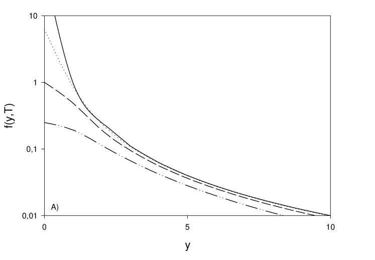
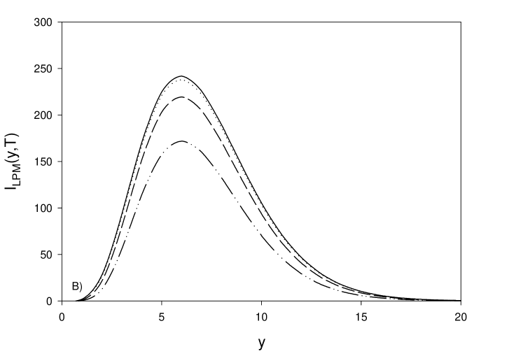
Figure 7: The functions $f(y,T)$ and $I_{LPM}(y,T)$ are shown at temperature $T=2$ MeV (dotted curve), $T=5$ Mev (dashed curve) and $T=10$ MeV (dashed-dotted curve). The QPA result is given by the solid line.

Finally we turn to the LPM effect. Clearly its possible relevance in the present case depends on the magnitude of the width $\Gamma$, which is a function of $\omega$, temperature T and density. Here we use the parameterization SD2000

$$\Gamma(\omega,T)=a(\frac{\omega^{2}}{4\pi^{2}}+T^{2})$$ (88)

to be able to estimate the importance of the LPM-effect. For $\omega<60MeV$ and $T<20MeV$, this roughly coincide within a factor 2 with Alm et al. Alm1996 . Including the LPM effect in the emissivity the function I(y) in Eq. (85) has to be replaced by

$$I_{LPM}(y,T)=y^{2}f(y,T)I(y)$$ (89)

with $f(y,T)=1/(y^{2}+\frac{\Gamma(yT,T)^{2}}{T^{2}})$, which can be derived from Eqs. (73), (78)and (83). The function $f(y,T)$ describes very roughly the behavior of $\Im m\Pi^{R}$. To give an indication of the importance of the LPM effect and to demonstrate the influence of the weighting factor in the emissivity we show in Fig. 7 how the functions $f(y,T)$ and $I_{LPM}(y,T)$ in Eq. (89) are modified for various values of the temperature. The value of the parameter $a$ depends weakly on the density and is approximately $0.2MeVc^{-1}$. One sees that the function $f(y,T)$ has a singularity at $y=0$ in the QPA. The LPM effect suppresses this infrared divergence. The function $I_{LPM}(y,T)$ is less sensitive to the LPM effect compared to the function $f(y,T)$, because the weighting factor in the emissivity strongly suppresses the $y=0$ contribution. Therefore the LPM effect in the emissivity is negligible for $T<5$ MeV. Comparing the ratio of the emissivity with and without LPM effect $R_{LPM}=\epsilon/\epsilon_{lpm}$ at $T=5$ MeV,$T=10$ MeV and $T=20$ MeV gives $0.89$,$0.68$ and $0.35$, respectively. The influence of the LPM-effect increases with temperature and becomes appreciable above $T=5$ MeV. Therefore in practice in calculating the emissivity the LPM effect does not play an important role for small $T$, say $T<5$ MeV.
Finally we note that an additional medium effect, not considered here, is the possible medium effect of the axial vector coupling $g_{A}$, which has been considered in CP2002 , where it is was found that space like axial coupling is quenched by about 20 percent. However the timelike axial coupling is not necessarily equal, since Lorentz invariance is broken. Experiments with first-forbidden $\beta$ decay of light nuclei give indications for an enhancement of the time-like axial charge of about 25 percent in the medium WTB1994 . This is in agreement with meson exchange calculations in the soft pion approximations T1992 .

V Summary and Conclusion

In this paper we studied the neutrino emissivity for the neutral current $NN$ bremsstrahlung process, relevant for neutron star cooling. In particular we considered some effects that are not included in the standard cooling scenario of FM1979 , which is based upon a non-relativistic quasi-particle approximation and the use of the one-pion exchange potential. The effects considered, namely the description of the $NN$ interaction, the LPM effect and relativistic effects, influence the neutrino emission of the neutral current bremsstrahlung process. Therefore these effects are expected to affect also other neutrino emission processes in a similar way.

First we studied how the description of the $NN$ interaction influences the $NN$ bremsstrahlung process. In the low density limit using the fact that $\omega$ is small the Low theorem Low can be applied, which allows us to use the on-shell $T$-matrix, specified by empirical phase shifts, and to compare it with OPE. At typical neutron momenta in neutron stars, approximately $300\ {\rm MeV}/{\rm c}$, the resulting free space cross section is roughly a factor 4-5 reduced compared to the application of OPE. Although adding ORE to OPE is an improvement, the result still differs a factor 2-3 with that obtained using the $T$-matrix. We also analyzed which Fermi components of the $T$-matrix dominate the rate, namely the tensor and the spin-orbit type terms.

To evaluate neutrino-pair bremsstrahlung in a finite medium at finite temperature we have used a closed diagram technique up to two loops. It is found that at $n\sim n_{0}$ the neutrino emissivity, applying the on-shell $T$-matrix to describe the $NN$ interaction, is roughly a factor 4 smaller than those based upon OPE. This is in qualitative agreement with the conclusion of Hanhart HPR2000 . Including medium effects from Pauli-blocking by replacing the T-matrix by a in-medium G-matrix,we find a small increase of the emissivity of 20-30 percent.

Secondly in order to investigate the many-body correlations we can go beyond QPA by considering dressed propagators with a temperature dependent imaginary part $\Gamma$. Of course gauge invariance of the vector current is conserved in our approach. In particular we find that in the medium the damping of the infrared divergence, the LPM effect, has a negligible effect for low temperatures ($T<5$ MeV); this is due to both the small single-particle width ($\Gamma\approx T^{2}$) and a weighting factor depending on $\omega$ in the phase space integral.

Finally we estimated relativistic (recoil) effects to be rather small, of the order of 10 percent, at nuclear saturation densities.

In short the description of the $NN$ interaction by the on-shell $T$-matrix OPE has the largest impact on the neutrino emission of the bremsstrahlung process; roughly a reduction factor of 4. Other effects are relatively small; below 30 percent for $T<5MeV$.

VI Acknowledgements

This work has been supported through the Stichting voor Fundamenteel Onderzoek der Materie with financial support from the Nederlandse Organisatie voor Wetenschappelijk Onderzoek. The work of J.A.T. is supported by the U.S. Department of Energy contract number DE-AC05-84ER40150 under which the Southeastern Universities Research Association (SURA) operates the Thomas Jefferson National Accelerator Facility. We thank R.G.E. Timmermans, and S. Reddy for helpful discussions.

Appendix A Neutrino transport

In the present paper we use the finite temperature real time Schwinger-Keldysh formalism to compute the collision integrals in the transport formalism. For the sake of completeness the main steps are summarized in this appendix; for more details we refer to SD2000 . In this formalism one must distinguish between vertices with indices (+) and (-). For given real interaction these are associated with the value $-iV$ (time ordered part) and with adjoint vertex $+iV$ (anti-time ordered part). The corresponding finite temperature Green functions (applied to neutrinos as well as the nucleons) can be expressed as a two times two matrix propagator:

$$i\underline{G}_{1,2}=\left(\begin{array}[]{cc}G^{--}_{12}&G^{-+}_{12}\\ G^{+-}_{12}&G^{++}_{12}\end{array}\right)=\left(\begin{array}[]{cc}\left<T\psi(x_{1})\bar{\psi}(x_{2})\right>&-\left<\bar{\psi}(x_{2})\psi(x_{1})\right>\\ \left<\psi(x_{1})\bar{\psi}(x_{2})\right>&\left<\tilde{T}\psi(x_{1})\bar{\psi}(x_{2})\right>\end{array}\right)$$ (94)

Sometimes it is more convenient to use the retarded and advanced functions:

$$i{G}^{R}_{12}=\theta(t_{1}-t_{2})\langle\left\{\psi(x_{1}),\overline{\psi}(x_{2})\right\}\rangle,\quad i{G}^{A}_{12}=\theta(t_{1}-t_{2})\langle\left\{\psi(x_{1}),\overline{\psi}(x_{2})\right\}\rangle,$$ (95)

The propagators satisfy the Dyson equation

$$\underline{G}(x_{1},x_{2})=\underline{G}_{0}(x_{1},x_{2})+\underline{G}_{0}(x_{1},x_{3})\underline{\Phi}(x_{3},x_{2})\underline{G}(x_{2},x_{1})$$ (96)

where $\underline{\Phi}$ is the proper self-energy.
Equivalently in integro-differential form

$$\not\!\partial_{1}\underline{G}_{1,2} = \delta_{1,2}\underline{\sigma}_{z}+\underline{\sigma}_{z}\int d3\underline{\Phi}_{13}\underline{G}_{3,2}$$ (97)

$$\not\!\partial_{2}^{*}\underline{G}_{1,2} = \delta_{1,2}\underline{\sigma}_{z}+\int d3\underline{G}_{1,3}\underline{\Phi}_{3,2}\sigma_{z},$$ (98)

where $\underline{\sigma}_{z}$ is the Pauli spin matrix. The semi-classical neutrino transport equation are obtained by subtracting the Dyson Eqs. (97) and (98) for $\partial_{1}$ and $\partial_{2}$

$$i\underline{G}(x_{1},x_{2})\not\!\partial_{x_{2}}-i\not\!\partial_{x_{1}}\underline{G}(x_{1},x_{2})$$

$$=\underline{G}(x_{1},x_{3})\underline{\Phi}(x_{3},x_{2})\underline{\sigma_{z}}-\underline{\sigma_{z}}\underline{\Phi}(x_{1},x_{3})\underline{G}(x_{3},x_{2}),$$ (99)

In particular the transport equation for the off-diagonal matrix Green function reads

$$\left[\not\!\partial_{x_{3}}-\Re e\,\Phi^{R}(x_{1},x_{3}),G^{+-,-+}(x_{3},x_{2})\right]-\left[\Re e\,G^{R}(x_{1},x_{2}),\Phi^{+-,-+}(x_{3},x_{2})\right]$$

$$=\frac{1}{2}\left\{G^{+-,-+}(x_{1},x_{3}),\Phi^{+-,-+}(x_{3},x_{2})\right\}+\frac{1}{2}\left\{\Phi^{+-,-+}(x_{1},x_{2}),G^{+-,-+}(x_{3},x_{2})\right\},$$ (100)

As a result of the assumption of the existence of the Lehmann representation we have $\Re eG^{R}=\Re eG^{A}=\Re eG$ and $\Re e\Phi^{R}=\Re e\Phi^{A}=\Re e\Phi$. The Wigner transforms of the off-diagonal Green functions correspond to Wigner densities in 4-coordinate and 4-momentum space. In the gradient expansion the Wigner transforms of convolution integrals can be expressed in terms of Poisson brackets $\{A,B\}_{P.B.}=\partial_{k}A\partial_{x}B-\partial_{x}A\partial_{k}B$. This leads to the quasi-classical neutrino transport equation in which the neutrino self-energies enter in the loss and gain terms

$$i\left\{\Re e\ G^{-1}(p,x),G^{+-,-+}(p,x)\right\}_{P.B.}+i\left\{\Re e\ G(p,x),\Phi^{+-,-+}(p,x)\right\}_{P.B.}$$

$$=G^{+-,-+}(p,x)\Phi^{+-,-+}(p,x)+\Phi^{+-,-+}(p,x)G^{+-,-+}(p,x),$$ (101)

The first Poisson bracket at the l.h.s. side leads (Vlasov part) to the Boltzmann drift term, whereas the second one corresponds to off-mass shell effects. After separating the pole and non-pole terms:

$$G^{+-,-+}(p,x)=G_{0}^{+-,-+}(p,x)+G_{\rm off}^{+-,-+}(p,x)$$

the quasiparticle part of the transport equation is given by

$$i\left\{\Re eG^{-1}(p,x),G_{0}^{+-,-+}(p,x)\right\}_{P.B.} = G^{+-,-+}(p,x)\Phi^{+-,-+}(p,x)$$ (102)

$$- \Phi^{+-,-+}(p,x)G^{+-,-+}(p,x),$$

where $\Re eG^{-1}(p,x)=\not\!\partial_{p}-\Re e\Phi^{R}(p,x)$. The l.h.s. corresponds to the drift term of the Boltzmann equation and the r.h.s. to the collision integrals. The remainder part of the transport equation

$$i\left\{\Re eG^{-1}(p,x).G_{off}^{+-,-+}(p,x)\right\}_{P.B.}+i\left\{\Re eG(p,x),\Phi^{+-,-+}(p,x)\right\}_{P.B.}=0$$ (103)

describes the off-shell effects, which we neglect.
The on-mass-shell neutrino propagator is related to the single-time distribution functions (Wigner functions) of neutrinos and anti-neutrinos, $f_{\nu}(q)$ and $f_{\bar{\nu}}(q)$,

$$G_{0}^{-+}(q,x)=\frac{i\pi\!\not\!q}{\omega(\vec{q})}\Big{[}\delta\left(q_{0}-\omega(\vec{q})\right)f_{\nu}(q,x)-\delta\left(q_{0}+\omega(\vec{q})\right)\left(1-f_{\bar{\nu}}(-q,x)\right)\Big{]}$$ (104)

and for the $G_{0}^{+-}$ propagator $f_{\nu}(q)$ replaced by 1- $f_{\nu}(q)$ and $1-f_{\bar{\nu}}(q)$ by $1-f_{\bar{\nu}}(q)$. In this limit the Boltzmann equation for the neutrino distributions is obtained

$$\left[\partial_{t}+\vec{\partial}_{q}\,\omega(\vec{q})\vec{\partial}_{x}\right]f_{\nu}(\vec{q},x) = \int_{0}^{\infty}\frac{dq_{0}}{2\pi}{\rm Tr}\Big{[}\Phi^{-+}(q,x)G_{0}^{+-}(q,x)$$ (105)

$$-\Phi^{+-}(q,x)G_{0}^{-+}(q,x)\Big{]}\equiv I^{-+}_{\nu}(\vec{q},x)-I^{+-}_{\nu}(\vec{q},x),$$

where the r.h.s. corresponds to the gain and loss term. (the Boltzmann Eq. for anti-neutrino follows by integration over the negative $q_{0}$).

Appendix B Collision integrals

In the lowest (second) order in the weak interaction the neutrino transport self-energies are given by

$$-i\Phi^{-+,+-}(q,x)=\int\frac{d^{4}q_{1}}{(2\pi)^{4}}\frac{d^{4}q_{2}}{(2\pi)^{4}}(2\pi)^{4}\delta^{4}(q_{1}+q_{2}-q)i\Gamma_{q_{1}}^{\mu}\,iG_{0}^{-+}(q_{2},x)i\Gamma_{q_{1}}^{\dagger\lambda}iS^{-+,+-}_{\mu\lambda}(q_{1},x),$$ (106)

where $S^{-+,+-}_{\mu\lambda}(q)$ is the baryon polarization tensor, and $\Gamma_{q}^{\mu}$ is the weak leptonic interaction vertex.
The collision integrals in Eq. (105), which are expressed as a convolution of the lepton self-energies $\Phi$ and the intermediate (anti-)neutrino propagator, consist of a sum of a loss and a gain term; e.g. the neutrino gain part

$$I_{\nu}^{-+}(\vec{q},x)=\int_{0}^{\infty}\frac{dq_{0}}{2\pi}{\rm Tr}[\Phi^{-+}(q,x)G_{0}^{+-}(q,x)]$$ (107)

contains a (space-like) scattering (proportional to $f_{\nu}(1-f_{\nu}))$ and a (time-like) pair emission term ($\propto(1-f_{\bar{\nu}})(1-f_{\nu}))$ The anti-neutrino one is obtained by replacing the positive energy range by the negative one.

Appendix C Finite $T$ hadronic Green functions

Although in the neutrino sector the stationary condition $\Phi^{-+}G^{+-}_{\nu}=\Phi^{+-}G^{-+}_{\nu}$ is not satisfied (see appendix), in the hadronic sector it is. Therefor the nucleons can be treated in the equilibrium Green function’s formalism. The retarded self energy $\Sigma^{R}$ can be decomposed in Lorentz components, in nuclear matter only the scalar and vector components are non zero

$$\Sigma^{R}(p)=\Sigma^{R}_{S}(p)+\!\not\!{\Sigma}^{R}_{V}(p)$$

with $p=(p^{0},\vec{p})$. The retarded relativistic dressed baryon Green function DP1991 is

$$G^{R}(p)=\frac{\!\not\!{p}+m-\!\not\!{\Sigma}^{R}_{V}(p)+\Sigma^{R}_{S}(p)}{(p-\Sigma^{R}_{V}(p)).(p-\Sigma^{R}_{V}(p))-(m+\Sigma^{R}_{S}(p))^{2}}$$ (108)

and the spectral function

$$A(p)=-2\Im mG^{R}(p).$$ (109)

Using Eqs. 108 and 109 we can now give the following relations

$$G^{-+}(p)=if(p^{0})A(p),$$ (110)

$$G^{+-}(p)=-i(1-f(p^{0}))A(p),$$ (111)

$$G^{--}(p)=(1-f(p^{0}))G^{R}(p)+f(p^{0})G^{A}(p),$$ (112)

$$G^{++}(p)=-(1-f(p^{0}))G^{A}(p)-f(p^{0})G^{R}(p)$$ (113)

with $f(p_{0})=1/\Big{(}\exp(\beta(p^{0}-\mu))+1\Big{)}$, $\beta=1/kT$ and the chemical potential $\mu=E_{p_{F}}+\Re e\Sigma^{0,R}_{V}(p_{F})$. We will now define the relativistic effective Dirac mass $m_{D}=m+\Re e\Sigma^{R}_{S}(p)$, $\tilde{p}^{0}=p^{0}-\Re e\Sigma^{0,R}(p)$, $\vec{\tilde{p}}=\vec{p}+\Re e\vec{\Sigma}^{R}_{V}(p)$ ,$\tilde{E}_{p}=\sqrt{(\vec{\tilde{p}})^{2}+(m_{D})^{2}}$ and $\Gamma=2\Im m\Big{(}-\Sigma^{0,R}_{V}-\frac{m_{D}}{\tilde{E}_{p}}\Sigma^{R}_{S}(p)+\frac{\vec{\tilde{p}}}{\tilde{E}_{p}}\vec{\Sigma}^{R}_{V}(p)\Big{)}$. We will consider two cases:i) the QPA Green functions: $\Im m\Sigma(p)\rightarrow 0$ and ii) the non-relativistic Green functions.

C.1 Green functions in QPA

In the QPA case, the imaginary part of self energy $\Im m\Sigma(p)$ vanishes. This gives the following definitions for the Green functions in Eqs. (110),(111), (112) and (113)

$$G_{0}^{+-}(p)=-2i\pi\frac{m_{D}\Lambda^{+}(\tilde{p})}{\tilde{p}^{0}}(1-f(p^{0}))\delta(\tilde{p}^{0}-\tilde{E}_{p}),$$ (114)

$$G_{0}^{-+}(p)=2i\pi\frac{m_{D}\Lambda^{+}(\tilde{p})}{\tilde{p}^{0}}f(p^{0})\delta(\tilde{p}^{0}-\tilde{E}_{p}),$$ (115)

$$G_{0}^{--}(p)=(G_{0}^{++}(p))^{*}=\frac{2m_{D}\Lambda^{+}(\tilde{p})}{\tilde{p}^{2}-m^{2}_{D}},$$ (116)

where we have the positive-energy operator $\Lambda^{+}(\tilde{p})=\frac{\!\not\!{\tilde{p}}+m_{D}}{2m_{D}}$ and $Z^{-1}_{F}(p)=\partial(\tilde{p}^{2}-m^{2}_{D})/\partial p^{0}$. The causal propagators $G_{0}^{--}$ and $G_{0}^{++}$ are off-mass-shall. If $\tilde{p}$ is on-mass-shell $\tilde{p}^{2}-{m_{D}}^{2}=0$, then $G^{--}$ can be rewritten as

$$G_{0}^{--}(p\pm q)=(G_{0}^{++}(p\pm q))^{*}=\frac{2m_{D}\Lambda^{+}(\tilde{p})}{\pm 2\tilde{p}.q}.$$ (117)

We point out that, when taking complex conjugates, it is understood that Dirac gamma matrices are not conjugated. The free case can easily be obtained from this. By replacing $m_{D}$,$\tilde{p}$ by $m$ and $p$ we obtain the free Green functions.

C.2 The non-relativistic Green functions

In this part will be given the non-relativistic Green functions. Besides the non-relativistic limit, we will assume that the width of the quasi-particle state, is small, $\Im m\Sigma^{R}(p)\ll\Re e\Sigma^{R}(p)$. We will now define the Green functions in the non-relativistic limit as

$$G^{-+}(p)=\frac{i\Gamma(p)}{(p^{0}-\eta_{\vec{p}})^{2}+\Gamma(p)^{2}/4}f(p^{0}),$$ (118)

$$G^{+-}(p)=\frac{-i\Gamma(p)}{(p^{0}-\eta_{\vec{p}})^{2}+\Gamma(p)^{2}/4}(1-f(p^{0}))$$ (119)

and

$$G^{--}(p)=(G^{++}(p))^{*}=\frac{p^{0}-\eta_{p}}{\left[p^{0}-\eta_{\vec{p}}\right]^{2}+\Gamma(p)^{2}/4}$$

$$-\frac{i\Gamma(p)}{\left[p^{0}-\eta_{\vec{p}}\right]^{2}+\Gamma(p)^{2}/4}{\rm tanh}\left(\frac{p^{0}}{2}\right),$$ (120)

where $\Gamma(p)=-2\Im m\Big{(}\Sigma^{0,R}_{V}(p)+\Sigma^{R}_{S}(p)\Big{)}$, ${\rm tanh}\left(p^{0}\right)=1-2f(2p^{0})$, and $\eta_{\vec{p}}=\epsilon^{0}_{\vec{p}}$ with $\epsilon^{0}_{\vec{p}}=|\vec{p}|^{2}/(2m^{*})$ and $m^{*}$ the non-relativistic effective mass.

References

• (1) B.L. Friman and O.V. Maxwell, Astrophys. J. 232, 541 (1979).
• (2) C. Hanhart, D.R. Philips, S. Reddy, Phys. Lett B499, 9 (2001).
• (3) R. Timmermans, A.Yu. Korchin, E.N.E. van Dalen and A.E.L. Dieperink, Phys. Rev. C65, 064007 (2002).
• (4) D.N. Voskresensky and A.V. Senatorov, Sov. Phys. JETP 63, 885 (1986).
• (5) J. Knoll and D.N. Voskresensky, Ann. Phys. 249, 532 (1996).
• (6) A. Sedrakian and A.E.L. Dieperink, Phys. Rev. D62, 083002(2000).
• (7) M.E. Gusakov, Astron. Astrophys. 389, 702 (2002)
• (8) D.G. Yakovlev, A.D. Kaminker, P. Haensel and O.Y. Gnedin, Astron. Astrophys. 389, L24 (2002)
• (9) F.E. Low, Phys. Rev. 110, 974 (1958).
• (10) M.L. Goldberger, M.T. Grisaru, S.W. MacDowell and D.Y. Wong, Phys. Rev. 120, 2250 (1960); M.L. Goldberger, Y. Nambu and R. Oehme, Ann. Phys. (N.Y.) 2, 726 (1957).
• (11) J.A. Tjon and S.J. Wallace, Phys. Rev. C32, 267 (1985).
• (12) V.G.J. Stoks, R.A.M. Klomp, M.C.M. Rentmeester and J.J. de Swart, Phys. Rev. C48, 792 (1993).
• (13) V.G.J. Stoks, R.A.M. Klomp, C.P.F. Terheggen, and J.J. de Swart, Phys. Rev. C49, 2950 (1994).
• (14) W. Botermans and R. Malfliet, Phys. Rep. 198, 115 (1990).
• (15) J.E. Davis and R. J. Perry, Phys. Rev. C43, 1893 (1991).
• (16) F. de Jong and R. Malfliet, Phys. Rev. C44, 998 (1991).
• (17) S. Reddy, M. Prakash, J.M. Lattimer and J.A. Pons, Phys. Rev. C59, 2888 (1999).
• (18) P. Aurenche, F. Gelis and H. Zaraket, Phys. Rev. D62, 096012 (2000).
• (19) J. Cleymans, V.V. Goloviznin, K. Redlich, Phys. Rev. D47, 989 (1993).
• (20) G. Raffelt, D. Seckel, Phys. Rev. D52, 1780 (1995).
• (21) M.K. Banerjee and J.A. Tjon, Phys.Rev. C58, 2120 (1998).
• (22) D. Blaschke, G. R$\ddot{\rm o}$pke, H. Schulz, A.D. Sedrakian and D.N. Voskresensky, Mon. Not. R. Astron. Soc. 273, 596 (1995).
• (23) M.K. Banerjee and J.A. Tjon, Nucl. Phys. A708, 303 (2002)
• (24) D.G. Yakovlev, A.D. Kaminker, O.Y. Gnedin and P. Haensel, Phys. Rep. 354, 1 (2001)
• (25) T. Alm, G. R$\ddot{\rm o}$pke, A. Schnell, N.H. Kwong and H.S. K$\ddot{\rm o}$hler, Phys. Rev. C53, 2181 (1996).
• (26) G.W. Carter and M. Prakash, Phys. Lett. B525, 249 (2002).
• (27) E.K. Warburton, I.S. Towner, B.A. Brown, Phys. Rev. C49, 824 (1994).
• (28) I.S. Towner, Nucl. Phys. A542, 631 (1992).