Nuclear response functions for the $\mathbf{N-N^{*}(1440)}$ transition

Abstract

Parity-conserving and -violating response functions are computed for the inclusive electroexcitation of the $N^{*}(1440)$ (Roper) resonance in nuclear matter modeled as a relativistic Fermi gas. Using various empirical parameterizations and theoretical models of the $N-N^{*}(1440)$ transition form factors, the sensitivity of the response functions to details of the structure of the Roper resonance is investigated. The possibility of disentangling this resonance from the contribution of $\Delta$ electroproduction in nuclei is addressed. Finally, the contributions of the Roper resonance to the longitudinal scaling function and to the Coulomb sum rule are also explored.

, , and

1 Introduction

Parity-conserving (PC) inclusive electron scattering from nuclei has attracted considerable attention as a probe of nuclear structure. Virtual photons penetrate deeply inside the nucleus allowing one to test modeling of various aspects of the nuclear many-body problem including effects from nuclear correlations, meson exchange currents and relativistic effects [1, 2]. Parity-violating (PV) electron scattering from nuclei — inclusive scattering of longitudinally polarized electrons — goes even further by opening the possibility of obtaining new information not only on nuclear, but also on nucleon structure, especially on the strangeness content of the nucleon. Indeed, a basic motivation for studying PV asymmetries in nuclei with polarized electrons is that scattering from a free proton alone is insufficient when attempting to disentangle all of nucleon’s form factors and somewhere a neutron (hence, a nucleus) must be involved [3].

Many studies have been focused on the energy region of the quasielastic (QE) peak and the $\Delta$ resonance [2, 4]. However, there is increasing interest in the so called second resonance region, namely where the $N^{*}(1440)P_{11}$ (Roper), $N^{*}(1520)D_{13}$ and $N^{*}(1535)S_{11}$ resonances are to be found. Understanding the properties of these $N-N^{*}$ transitions is a challenge for quark models and relates to basic issues such as the nature of quark-hadron duality and the roles played by gluons in the baryon excitation spectrum. The experimental study of meson electroproduction on the proton, currently underway at JLab, is presently providing data in this region [5, 6]. Similar studies in nuclei would add information on the in-medium dynamics of these resonances and on possible modifications of baryon properties inside the nucleus [7].

The $N^{*}(1440)P_{11}$ is one of the most puzzling of the resonances occurring just above the $\Delta$(1232). It is usually viewed as a radial excitation of a three-quark nucleon state — a breathing mode. However, the standard non-relativistic constituent quark modeling fails to describe all of its properties, in particular its mass which is overestimated. This outcome has prompted further studies, pointing to the relevance of chiral symmetry [8], relativistic corrections [9], meson clouds [9, 10] or configuration mixing due to gluon exchange [11]. Alternative approaches describe the Roper as a Skyrme soliton [12, 13], a hybrid state with a large gluonic component [14], a nucleon-sigma molecule [15] or as a chiral soliton within the chromodielectric model [16]. All of these models predict specific behaviors for the electroproduction amplitudes $A^{p,n}_{1/2}$, $S^{p,n}_{1/2}$, which, in turn, have consequences for the nuclear response functions. The experimental information available so far comes from the multipole analysis of Gerhardt [17] and is clearly insufficient to allow a stringent test of these theories. It is also worth mentioning the relevant role played by the $N^{*}(1440)$ in the description of several hadronic reactions at intermediate energies, $\pi N\rightarrow\pi\pi N$ [18], $NN\rightarrow NN\pi\pi$ [19] and especially the $(\alpha,\alpha^{\prime})$ reaction on a proton target where the isoscalar excitation of the Roper clearly stands out in the data [20, 21].

The aim of this work is to make a first step towards a theoretical description of the nuclear response functions (both parity-conserving and -violating) in the second resonance region. We calculate these responses for the Roper resonance excitation in nuclei using the simple (perhaps oversimplified, but at least respecting Lorentz and gauge invariance) Relativistic Fermi Gas (RFG) model [22]. The paper is organized as follows: first we consider the PC response and, after discussing the general formalism, we calculate the RFG response functions in the domain of the $N-N^{*}(1440)$ transition using for this form factors related to the helicity amplitudes. We present results corresponding to various parameterizations and model calculations of the Roper’s structure available in the literature, emphasizing their specific impacts on the nuclear response functions. Next we explore the consequences of including the Roper excitation on the scaling and superscaling properties of the nuclear response functions and on the Coulomb sum rule. Finally, we perform a similar investigation in the PV case.

2 Parity-conserving response functions

2.1 General formalism

We consider the scattering of an electron with initial and final four-momenta $k=(E,\mathbf{k})$ and $k^{\prime}=(E^{\prime},\mathbf{k}^{\prime})$, respectively, from a nucleus. The momentum transferred to the latter, namely $q=k-k^{\prime}=(\omega,\mathbf{q})$, is carried by a single virtual photon. As in past work, the set of dimensionless variables

$$\kappa=(\lambda,\boldsymbol{\kappa})=\left(\frac{\omega}{2m_{\scriptscriptstyle{N}}},\frac{\mathbf{q}}{2m_{\scriptscriptstyle{N}}}\right)\,,\quad\tau=\boldsymbol{\kappa}^{2}-\lambda^{2}=-\frac{q^{2}}{4m^{2}_{\scriptscriptstyle{N}}}=\frac{|Q^{2}|}{4m^{2}_{\scriptscriptstyle{N}}}$$ (1)

$$\eta=(\epsilon,\boldsymbol{\eta})=\left(\sqrt{1+\frac{\mathbf{p}^{2}}{m_{\scriptscriptstyle{N}}^{2}}},\ \frac{\mathbf{p}}{m_{\scriptscriptstyle{N}}}\right)\,,$$ (2)

$$\eta_{\scriptscriptstyle{F}}=\frac{k_{\scriptscriptstyle{F}}}{m_{\scriptscriptstyle{N}}}\,,\quad\epsilon_{\scriptscriptstyle{F}}=\sqrt{1+\eta_{\scriptscriptstyle{F}}^{2}}\,,\quad\xi_{\scriptscriptstyle{F}}=\epsilon_{\scriptscriptstyle{F}}-1$$ (3)

($m_{\scriptscriptstyle{N}}$ being the nucleon mass and $k_{\scriptscriptstyle{F}}$ the Fermi momentum) for the nucleon is used.

In the Born approximation and in the ultra-relativistic limit ($m_{e}\rightarrow 0$), the inclusive differential cross section reads [23]

$$\frac{d\sigma}{d\Omega^{\prime}dE^{\prime}}=\sigma_{\scriptscriptstyle{M}}\frac{1}{2EE^{\prime}\cos^{2}{\theta_{e}/2}}L_{\mu\nu}W^{\mu\nu}=\sigma_{\scriptscriptstyle{M}}\left(v_{\scriptscriptstyle{L}}R^{\scriptscriptstyle{L}}+v_{\scriptscriptstyle{T}}R^{\scriptscriptstyle{T}}\right)\,,$$ (4)

$\sigma_{\scriptscriptstyle{M}}$ being the Mott cross section, $\theta_{e}$ the electron scattering angle and $R^{{\scriptscriptstyle{L}}({\scriptscriptstyle{T}})}$ the longitudinal (transverse) response functions. The kinematical factors $v_{{\scriptscriptstyle{L}}({\scriptscriptstyle{T}})}$ are

$$v_{\scriptscriptstyle{L}}=\frac{\tau^{2}}{\boldsymbol{\kappa}^{4}}\,,\quad v_{\scriptscriptstyle{T}}=\frac{\tau}{2\boldsymbol{\kappa}^{2}}+\tan^{2}{\frac{\theta_{e}}{2}}$$ (5)

and the leptonic tensor $L_{\mu\nu}$ is

$$L_{\mu\nu}=\frac{1}{4}\mathrm{Tr}\left[k\!\!\!/\gamma_{\mu}k^{\prime}\!\!\!\!/\gamma_{\nu}\right]=k_{\mu}k^{\prime}_{\nu}+k^{\prime}_{\mu}k_{\nu}-g_{\mu\nu}k\cdot k^{\prime}\,.$$ (6)

The response functions are connected to the nuclear tensor according to the following relations

$$R^{\scriptscriptstyle{L}}=W^{00}\,,\quad R^{\scriptscriptstyle{T}}=W^{11}+W^{22}\,.$$ (7)

In our case, $W^{\mu\nu}$ accounts for the $N-N^{*}(1440)$ transition inside the nucleus. Analogously to the case of the $N-\Delta$ transition [24], it is given by

$$W^{\mu\nu}=\int^{\mu^{*}_{max}}_{\mu^{*}_{min}}d\mu^{*}G(\mu^{*})W_{0}^{\mu\nu}(\mu^{*})\,,$$ (8)

where $\mu^{*}$, the ratio between the Roper invariant mass W and the nucleon mass, ranges from $\mu^{*}_{min}=1+(m_{\pi}/m_{\scriptscriptstyle{N}})$ to $\mu^{*}_{max}=\sqrt{(\epsilon_{\scriptscriptstyle{F}}+2\lambda)^{2}-(\eta_{\scriptscriptstyle{F}}-2|\boldsymbol{\kappa}|)^{2}}$. Moreover, we parametrize the spectral function of the Roper resonance in the form

$$G(\mu^{*})=\frac{1}{2\pi}\frac{\Gamma(W)/m_{\scriptscriptstyle{N}}}{\left(\mu^{*}-m^{*}/m_{\scriptscriptstyle{N}}\right)^{2}+\Gamma^{2}(W)/(4m^{2}_{\scriptscriptstyle{N}})}\,,$$ (9)

where $m^{*}=1440$ MeV is the resonance mass and $\Gamma(W)$ its total width. Our specific expression for this energy-dependent total width is given in the Appendix. Finally, $W_{0}^{\mu\nu}(\mu^{*})$ is the standard RFG tensor associated with a narrow $N^{*}$ of mass $W=m_{\scriptscriptstyle{N}}\mu^{*}$, namely

$$W_{0}^{\mu\nu}(\mu^{*})=\frac{3{\mathcal{N}}}{4|\boldsymbol{\kappa}|m_{\scriptscriptstyle{N}}\eta_{F}^{3}}\int_{\epsilon_{0}}^{\epsilon_{F}}f^{\mu\nu}(\epsilon,\mu^{*})d\epsilon\,,$$ (10)

where

$$\epsilon_{0}=|\boldsymbol{\kappa}|\sqrt{1/\tau+\rho^{2}}-\lambda\rho$$ (11)

is the minimum energy of the struck nucleon as a function of $|\boldsymbol{\kappa}|$, $\lambda$ and the inelasticity parameter $\rho$, which is defined as [24]

$$\rho=1+\frac{1}{4\tau}(\mu^{*2}-1)\,.$$ (12)

The particle number ${\mathcal{N}}$ corresponds to the proton and neutron number, respectively. The nuclear responses are clearly obtained by adding the contributions from the two species, with weightings ${\mathcal{N}}=Z$ and ${\mathcal{N}}=N$, respectively.

Concerning the single-nucleon tensor $f_{\mu\nu}$, its standard form is given by [3]

$$f^{\mu\nu}=-w_{1}(\tau,\mu^{*})\left(g^{\mu\nu}+\frac{\kappa^{\mu}\kappa^{\nu}}{\tau}\right)+w_{2}(\tau,\mu^{*})V^{\mu}V^{\nu}\,,$$ (13)

where $V_{\mu}=\eta_{\mu}+\kappa_{\mu}\rho$. The insertion of Eq. (13) into Eq. (10) leads then to the following expressions for the longitudinal and transverse response functions

$$R^{{\scriptscriptstyle{L}}({\scriptscriptstyle{T}})}(|\mathbf{q}|,\omega)=\int^{\mu^{*}_{max}}_{\mu^{*}_{min}}d\mu^{*}G(\mu^{*})R_{0}^{{\scriptscriptstyle{L}}({\scriptscriptstyle{T}})}(|\mathbf{q}|,\omega,\mu^{*})\,,$$ (14)

where

$$R_{0}^{{\scriptscriptstyle{L}}({\scriptscriptstyle{T}})}(|\mathbf{q}|,\omega,\mu^{*})=\frac{3{\mathcal{N}}}{4|\boldsymbol{\kappa}|m_{\scriptscriptstyle{N}}\eta_{\scriptscriptstyle{F}}^{3}}\xi_{\scriptscriptstyle{F}}\,\Theta(1-\psi^{*2})(1-\psi^{*2})U^{\scriptscriptstyle{L}(\scriptscriptstyle{T})}(|\mathbf{q}|,\omega,\mu^{*})$$ (15)

with

$$U^{\scriptscriptstyle{L}} = \frac{\boldsymbol{\kappa}^{2}}{\tau}\left[(1+\tau\rho^{2})w_{2}(\tau,\mu^{*})-w_{1}(\tau,\mu^{*})+w_{2}(\tau,\mu^{*}){\mathcal{D}}(\kappa,\mu^{*})\right]\,,$$ (16)

$$U^{\scriptscriptstyle{T}} = 2w_{1}(\tau,\mu^{*})+w_{2}(\tau,\mu^{*}){\mathcal{D}}(\kappa,\mu^{*})\,,$$ (17)

$${\mathcal{D}}(\kappa,\mu^{*}) = \frac{\tau}{\boldsymbol{\kappa}^{2}}\left[(\lambda\rho+1)^{2}+(\lambda\rho+1)(1+\psi^{*2})\xi_{\scriptscriptstyle{F}}+\frac{1}{3}(1+\psi^{*2}+\psi^{*4})\xi_{\scriptscriptstyle{F}}^{2}\right]$$ (18)

$$- (1+\tau\rho^{2})\,.$$

Moreover,

$$\psi^{*2}=\frac{\epsilon_{0}-1}{\xi_{\scriptscriptstyle{F}}}\,$$ (19)

is the squared scaling variable associated with the resonance. The above expressions are independent of the specific transition under consideration: they can be used to describe the $\Delta$ region (after replacing $m^{*}$ by $m_{\Delta}$ in Eq. (9) and modifying $\Gamma(W)$ accordingly) as well as the quasielastic peak (in the $\Gamma\rightarrow 0$ limit setting $m^{*}=m_{\scriptscriptstyle{N}}$) [3, 24, 25]. In other words, all of the information about the $N-N^{*}(1440)$ transition is embedded in the functions $w_{1,2}(\tau,\mu^{*})$. In order to relate these to the transition form factors (and to the helicity amplitudes), we need to write $f^{\mu\nu}$ in terms of the $N-N^{*}(1440)$ electromagnetic current.

2.2 Hadronic tensor and form factors

The $N-N^{*}(1440)$ tensor reads

$$f^{\mu\nu}=\frac{1}{2}\mu^{*}\mathrm{Tr}\left[\frac{(p\!\!\!\!\>/+m_{\scriptscriptstyle{N}})}{2m_{\scriptscriptstyle{N}}}\left(\gamma_{0}J^{\dagger\mu}\gamma_{0}\right)\frac{(p\!\!\!\!\>/^{\prime}+W)}{2W}J^{\nu}\right]\,,$$ (20)

where the spinor matrix element of the current, written in terms of form factors and gauge invariant operators [26, 27, 28], is given by

$$J^{\alpha}=\bar{u}_{N^{*}}(p^{\prime})\left[F_{1}(q^{2})\left(q\!\!\!\!\>/\,q^{\alpha}-q^{2}\gamma^{\alpha}\right)+iF_{2}(q^{2})\sigma^{\alpha\beta}q_{\beta}\right]u(p)\,.$$ (21)

Notice the structure of the current which is very similar to its nucleonic counterpart (but for obvious redefinitions of the form factors) except for the $q\!\!\!\!\,/\,q^{\alpha}$ part. For the nucleon, the form factor associated with this operator has to vanish to ensure current conservation, but not for the Roper, since the mass of the latter differs from that of the nucleon.

Substituting Eq. (21) into Eq. (20) and casting the result in the form of Eq. (13), one gets $w_{1,2}$ in terms of the form factors according to

$$w_{1} = \displaystyle\left[\tau+\frac{(\mu^{*}-1)^{2}}{4}\right]G_{\scriptscriptstyle{M}}^{2}\,,$$ (22)

$$w_{2} = \displaystyle\frac{1}{\displaystyle 1+\frac{4\tau}{(\mu^{*}+1)^{2}}}\left[G_{\scriptscriptstyle{E}}^{2}+\frac{4\tau}{(\mu^{*}+1)^{2}}G_{\scriptscriptstyle{M}}^{2}\right]\,,$$ (23)

where $G_{\scriptscriptstyle{E},\scriptscriptstyle{M}}$ are defined analogously to the Sachs form factors of the nucleon [11, 27], i.e.,

$$G_{\scriptscriptstyle{E}} = \displaystyle 4m_{\scriptscriptstyle{N}}^{2}\tau\left[F_{1}-\frac{F_{2}}{m_{\scriptscriptstyle{N}}(\mu^{*}+1)}\right]\,,$$ (24)

$$G_{\scriptscriptstyle{M}} = \displaystyle 4m_{\scriptscriptstyle{N}}^{2}\tau F_{1}+m_{\scriptscriptstyle{N}}(\mu^{*}+1)F_{2}\,.$$ (25)

Indeed, when $\mu^{*}\rightarrow 1$, Eqs. (22,23) coincide with the well-known expressions for the nucleon (see for instance [3]).

2.3 Helicity amplitudes

Electromagnetic transitions between a nucleon and a resonant state are often expressed as helicity amplitudes, which describe transitions between a nucleon state with helicity $\lambda=1/2$ and a resonant state with $\lambda^{\prime}=1/2$ or $3/2$. In the case of the Roper two helicity amplitudes $A_{1/2}$ and $S_{1/2}$ should be introduced. They are defined as [27]

$$A_{1/2}^{p(n)}(Q^{2}) = \sqrt{\frac{2\pi\alpha}{k_{R}}}{\bigl{\langle}N^{*}\downarrow\bigr{|}}\epsilon^{\scriptscriptstyle(+)}_{\mu}J^{p(n)\mu}{\bigl{|}N\uparrow\bigr{\rangle}}\,,$$ (26)

$$S_{1/2}^{p(n)}(Q^{2}) = \sqrt{\frac{2\pi\alpha}{k_{R}}}\frac{|{\mathbf{q}|}}{Q^{2}}{\bigl{\langle}N^{*}\uparrow\bigr{|}}\epsilon^{\scriptscriptstyle(0)}_{\mu}J^{p(n)\mu}{\bigl{|}N\uparrow\bigr{\rangle}}\,,$$

where $\alpha$ is the electromagnetic fine-structure constant, $k_{R}$ is the energy of a real photon equivalent to the virtual one and $\epsilon^{\scriptscriptstyle(+,0)}$ stand for the transverse and longitudinal polarizations of the virtual photon. Inserting Eq. (21) in the above expressions and using the definitions of $G_{\scriptscriptstyle E,M}$ given in Eqs. (24, 25), it is straightforward to relate the helicity amplitudes to the form factors [11, 28] according to

$$A^{p(n)}_{1/2}(\tau) = f(\tau,\mu^{*})G^{p(n)}_{\scriptscriptstyle{M}}(\tau,\mu^{*})\,,$$ (27)

$$S^{p(n)}_{1/2}(\tau) = f(\tau,\mu^{*})\frac{\sqrt{[(\mu^{*}-1)^{2}+4\tau][(\mu^{*}+1)^{2}+4\tau]}}{8\sqrt{2}\tau}\,\times$$ (28)

$$\frac{\mu^{*}+1}{\mu^{*}}G^{p(n)}_{\scriptscriptstyle{E}}(\tau,\mu^{*})\,,$$

with

$$f(\tau,\mu^{*})=\sqrt{\frac{2\pi\alpha}{m_{\scriptscriptstyle{N}}}\frac{(\mu^{*}-1)^{2}+4\tau}{\mu^{*2}-1}}\,.$$ (29)

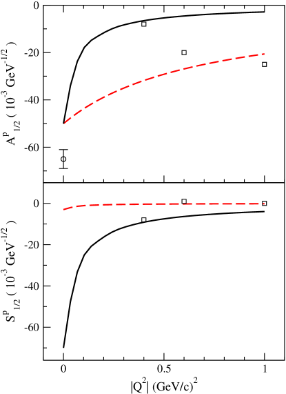
Figure 1: $N-N^{*}(1440)$ helicity amplitudes as a function of $|Q^{2}|$ for two different fits, Gh1 (solid lines) and Gh2 (dashed lines), of the data [17, 14]. The squares are the results of Gerhardt’s analysis at fixed energies and the circle is the value at the photon point [29].

As already mentioned, the only well established experimental information about these amplitudes was obtained by Gerhardt from a partial wave analysis of the data taken at NINA and DESY [17]. A fit in the second resonance region was performed independently at three fixed values of $Q^{2}$ and in the whole range (0-1 (GeV$/c$)²) for all of the NINA and DESY data separately. The results, converted into helicity amplitudes from the original $M_{1-}$ and $S_{1-}$ multipoles by Li et al. [14], are shown in Fig. 1. These amplitudes are for the $p-p^{*}(1440)$ transition; there is no information on the $Q^{2}$-dependence of the neutron form factors and only the value at the photon point ($Q^{2}=0$) is known [29]. One should also bear in mind that the analysis includes model-dependent assumptions; the systematic error is estimated to be no smaller than $\pm 12\times 10^{-3}$ GeV^-1/2 [14]. On the positive side, the preliminary result of an analysis of the pion electroproduction data measured in the CLAS detector at JLab at the $|Q^{2}|=0.4$ (GeV$/c$)² is in excellent agreement with Gerhardt’s value [5].

The $N-N^{*}(1440)$ transition amplitudes have been studied using various models with a wide diversity of results. Some of these are shown in Fig. 2, namely, the prediction from the non-relativistic quark model (NRQM) [14], the hybrid model [14], the light-front relativistic quark model (LF) calculation of [11], the chiral chromodielectric (ChD) model (self-consistent calculation) [16] and the extended vector-meson dominance (EVMD) model of [10] ($V_{I}$ potential). Notice that the hybrid model predicts $S^{p}_{1/2}=0$, whereas $S^{n}_{1/2}=0$ is obtained for both the NRQM and hybrid model. The chromodielectric model also yields an $S^{n}_{1/2}$ consistent with zero.

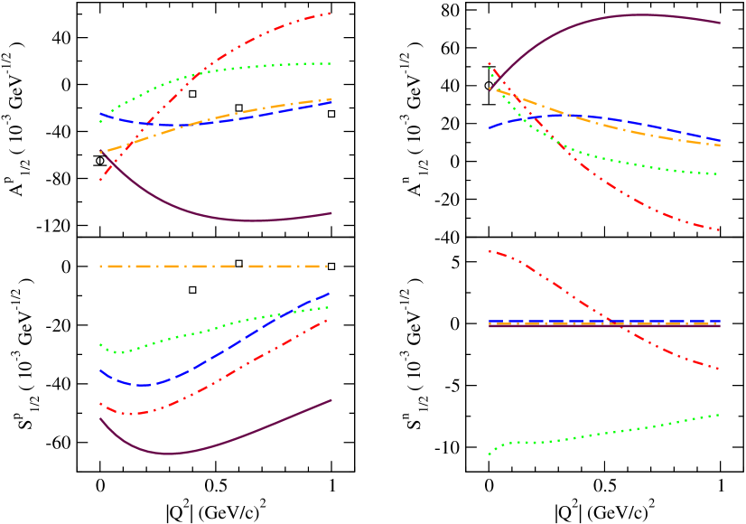
Figure 2: Transverse ($A_{1/2}$) and longitudinal ($S_{1/2}$) electroproduction amplitudes for the $N^{*}(1440)$ calculated with various models: NRQM (solid line) [14], hybrid model (dash-dotted line) [14], LF (dotted line) [11], ChD (dashed line) [16] and EVMD (dash-double-dotted line) [10].

2.4 Results and discussion

The RFG PC $N-N^{*}(1440)$ response functions are shown in Fig. 3 for two values of the transferred 3-momentum using the two empirical parameterizations for the helicity amplitudes displayed in Fig. 1. Since there are no measurements on the neutron, we assume the NRQM relations

$$A^{n}_{1/2}=-\frac{2}{3}A^{p}_{1/2}\,,\quad S^{n}_{1/2}=0\,.$$ (30)

The choice of $k_{\scriptscriptstyle{F}}=225$ MeV$/c$ and $Z=N=6$ corresponds to ¹²C. The contribution of the $\Delta$, as calculated in [24], has also been included. The total RFG response will thus arise, in first approximation, from the sum of the Roper and the $\Delta$ contributions. In the case of the transverse response, the Roper’s effect is negligible compared with that of the $\Delta$ at all energies. This does not come as surprise, since the strong $N-\Delta$ $M1$ transition appears at full strength in this observable. However, in the longitudinal channel the situation is different: the leading terms cancel [24, 25], which results in a longitudinal $\Delta$ response an order of magnitude smaller than the transverse one, giving a chance for other mechanisms to show up. Indeed, in the upper panels of Fig. 3, the Roper contribution appears as a moderately sharp peak at the edges of the spectra. Its size depends strongly on the parameterization of the helicity amplitudes. However, it should be kept in mind that near the light-cone the kinematical factor $v_{\scriptscriptstyle{L}}$ severely quenches the longitudinal channel, and hence it is doubtful if the Roper can be detected in this domain.

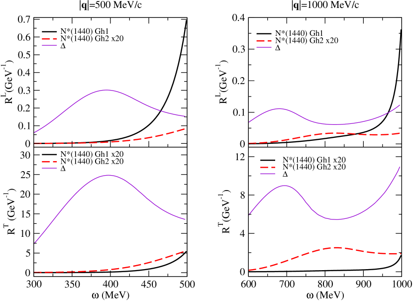
Figure 3: PC $N-N^{*}(1440)$ response functions for ¹²C at two values of the transferred 3-momentum and for two different parameterizations of the helicity amplitudes, Gh1 and Gh2 (see Fig. 2). The $N-\Delta$ responses are also shown. Notice that some curves have been multiplied by a factor 20 to make them visible.

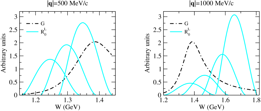
Figure 4: Combined plot of $G$ and $R_{0}^{\scriptscriptstyle{L}}$ functions as a function of the $N^{*}$ invariant mass. $R_{0}^{\scriptscriptstyle{L}}$ is shown at various $\omega$’s which are, from left to right, 400, 450 and 500 MeV on the left panel and 750, 830, 930 and 1000 MeV on the right panel.

Be it as it may, in order to understand the behavior of the Roper response near the light-cone, we have plotted the spectral function $G$ [see Eq. (9)] and $R_{0}^{\scriptscriptstyle{L}}$ as a function of the $N^{*}$ invariant mass in Fig. 4. Their convolution for a given $\omega$ value yields the response according to Eq. (14). Here we have used the parameterization Gh2 (dashed lines in Figs. 1 and 3). At larger values of $\omega$, $R_{0}^{\scriptscriptstyle{L}}$ probes higher invariant masses — hence its value at the maximum increases. At $|\mathbf{q}|=500$ MeV$/c$, the regions of higher $R_{0}^{\scriptscriptstyle{L}}$ correspond to larger $G$ values, producing a monotonic rise of $R^{\scriptscriptstyle{L}}$ as seen in the upper left panel of Fig. 3. The situation is completely different at $|\mathbf{q}|=1000$ MeV$/c$ where small $R_{0}^{\scriptscriptstyle{L}}$ and large $G$ are combined to produce a local maximum around $\omega=830$ MeV (see the dashed line in the upper right panel of Fig. 3) followed by a very shallow minimum around $930$ MeV; then, the rapid growth of $R_{0}^{\scriptscriptstyle{L}}$ compensates the decrease of $G$ at the edge of the spectrum.

Further information can be extracted from Fig. 4. At $|\mathbf{q}|=1000$ MeV$/c$ and for large values of $\omega$, where the Roper contribution might be significant, the relevant values of $W$ are well above the Roper peak. Therefore the response functions will not be dominated by the $\Delta$ and the Roper alone. Indeed many heavier resonances will contribute, making unreliable the information about the $N-N^{*}(1440)$ transition obtained on the basis of the data at this value of $|\mathbf{q}|$. However, at $|\mathbf{q}|=500$ MeV$/c$, the relevant values of $W$ are below $1.44$ GeV. It is then plausible to assume that the contribution of resonances heavier than the Roper is small, so that, relying on our present knowledge of the $N-\Delta$ transition, useful information about the Roper can eventually be obtained.

It is instructive to take a closer look at the responses in the light-cone limit ($\omega\rightarrow|\mathbf{q}|$, i.e., $\tau\rightarrow 0$; note that this limit is actually unobtainable for inelastic electron scattering even when the scattering angle approaches zero). A straightforward calculation yields

$$U^{\scriptscriptstyle{L}}(\lambda\rightarrow|\boldsymbol{\kappa}|) = \left(\frac{m_{\scriptscriptstyle{N}}}{2\pi\alpha}\right)\left[8\boldsymbol{\kappa}^{2}\frac{\mu^{*2}}{\mu^{*2}-1}S_{1/2}^{2}(0)+|\boldsymbol{\kappa}|\xi_{\scriptscriptstyle{F}}(1-\psi_{0}^{2})A_{1/2}^{2}(0)\right]\,,$$ (31)

$$U^{\scriptscriptstyle{T}}(\lambda\rightarrow|\boldsymbol{\kappa}|) = \left(\frac{m_{\scriptscriptstyle{N}}}{2\pi\alpha}\right)\frac{1}{2}(\mu^{*2}-1)A_{1/2}^{2}(0)\,,$$ (32)

with

$$\psi_{0}^{2}=\frac{(\mu^{*2}-1-4|\boldsymbol{\kappa}|)^{2}}{8\xi_{\scriptscriptstyle{F}}(\mu^{*2}-1)|\boldsymbol{\kappa}|}\,.$$ (33)

The insertion of the relevant numbers in Eq. (31) reveals the fact that the factor in front of $A_{1/2}^{2}(0)$ is about two orders of magnitude smaller than the one in front of $S_{1/2}^{2}(0)$ (notice the smallness of $\xi_{\scriptscriptstyle{F}}=0.03$). Therefore, the peak observed at the edge of the longitudinal response function is completely dominated by the $S_{1/2}$ amplitude evaluated close to the origin. It is then obvious that the different values for $S^{p}_{1/2}$ close to the origin predicted by Gh1 and Gh2 fits (lower panel in Fig. 1) are responsible for the large differences in the corresponding longitudinal response observed in Fig. 3. By the same argument, Eq. (32) and the upper panel of Fig. 1 explain why the transverse responses using the two parameterizations coincide as $\omega\rightarrow|\mathbf{q}|$, the curve obtained with Gh1 being above the other in the vicinity of this point.

Finally, we present the electromagnetic responses at $|\mathbf{q}|=500$ MeV$/c$ calculated with the helicity amplitudes obtained from the various models shown in Fig. 2. As expected from the above discussion, the size of the peak of the longitudinal response is determined by the strength of $S_{1/2}$ at $Q^{2}\rightarrow 0$. There is a big gap between the large result obtained with the NRQM and the almost negligible one found for the hybrid model where $S^{p}_{1/2}=S^{n}_{1/2}=0$. Notice also that the pattern is completely different in the case of $R^{\scriptscriptstyle{T}}$.

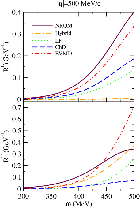
Figure 5: Electromagnetic $N-N^{*}(1440)$ responses at $|\mathbf{q}|=500$ MeV$/c$ calculated using the helicity amplitudes from the models displayed in Fig. 2.

3 Scaling behavior of the Roper responses

Study of the scaling properties of the cross sections and response functions in inclusive electron scattering provides important information about what constitute the relevant reaction mechanisms in the nucleus [30, 31]. This access to scaling is achieved by dividing the response functions by a function such that the physics related to the quasifree (elastic) scattering process on a single (moving) nucleon is removed. In this way, contributions from other mechanisms such as resonance excitation and meson exchange currents, which in general do not scale, can be revealed.

Our aim in this section is to investigate the scale-breaking effects associated with the excitation of the Roper resonance. For this purpose, we have computed the scaling functions

$$f_{\scriptscriptstyle{L(T)}}=k_{\scriptscriptstyle{F}}\frac{R_{\scriptscriptstyle{L(T)}}}{G_{\scriptscriptstyle{L(T)}}}$$ (34)

as a function of the QE scaling variable $\psi$ [3], which can be easily obtained from $\psi^{*}$ of Eqs. (19,11) by taking $\rho\rightarrow 1$. The response functions $R_{\scriptscriptstyle{L(T)}}$ are given by the sum of contributions from the quasi-elastic peak (taken from [3]) and the excitation of the $\Delta$ and Roper resonances. The functions $G_{\scriptscriptstyle{L(T)}}$ correspond essentially to the single-nucleon content of the nuclear responses. We take them as follows

$$G_{\scriptscriptstyle{L}} = \frac{|\boldsymbol{\kappa}|}{2\tau}\left[ZG^{2}_{\scriptscriptstyle{Ep}}+NG^{2}_{\scriptscriptstyle{En}}\right]$$ (35)

$$G_{\scriptscriptstyle{T}} = \frac{\tau}{|\boldsymbol{\kappa}|}\left[ZG^{2}_{\scriptscriptstyle{Mp}}+NG^{2}_{\scriptscriptstyle{Mn}}\right]\,.$$ (36)

This choice differs slightly from the one employed in [31] (Eqs. 16-19) in that the (small) medium corrections included there are disregarded here.

In Fig. 6 we display our results for $f_{\scriptscriptstyle{L}}$ at $|\mathbf{q}|=500$ and $1000$ MeV$/c$ and $\psi>1$, i.e., above the quasielastic region where resonance excitation is important. As expected, violations of both first- and second-kind scaling appear to set in. Above the $\Delta$ peak, the Roper contribution to the scaling violation in the longitudinal channel becomes important compared with that from the $\Delta$, at least in the case when the Gh1 parameterization is used, although the overall size of the effect is tiny (we recall that $f_{\scriptscriptstyle{L}}\simeq 0.7$ at $\psi=0$).

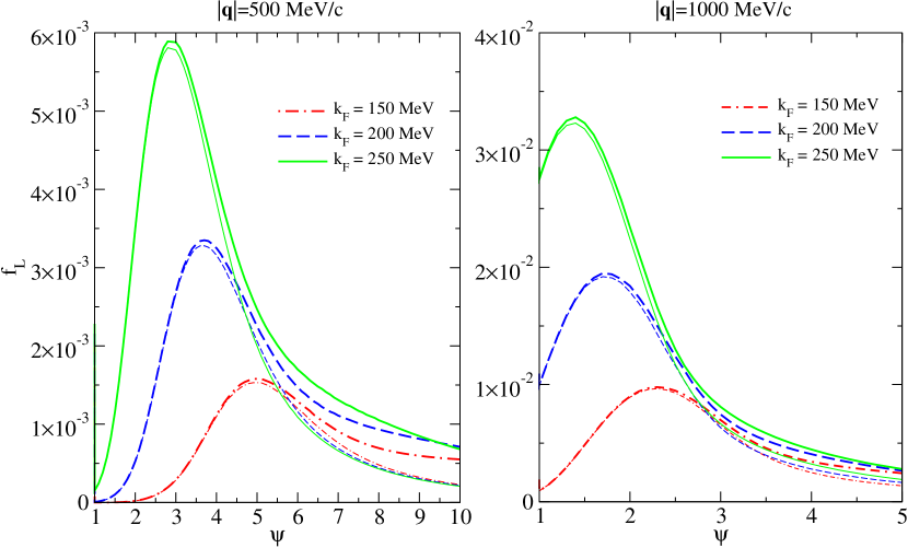
Figure 6: The longitudinal scaling function in resonance region, including the contributions of $\Delta$ alone (thin lines) and of the $\Delta$+Roper (thick lines) for $|\mathbf{q}|=500$ and 1000 MeV$/c$ and three values of $k_{\scriptscriptstyle{F}}$. The $N^{*}$ contribution is computed using the Gh1 parameterization.

Our findings of small scaling violation effects in the longitudinal channel is consistent with the experimental indications that $f_{\scriptscriptstyle{L}}$ exhibits superscaling behavior even above the quasielastic peak [32, 31]. The scaling violation is much more important in the transverse channel, but there the impact of the Roper is negligible compared with that of the $\Delta$.

4 Resonance contribution to the Coulomb sum rule

In this section, we investigate the contribution of the low-lying baryonic resonances $\Delta$ and $N^{*}(1440)$ to the integrated longitudinal response function, i.e. to the Coulomb sum rule. For this purpose, we compute the following ratio

$$\mathcal{R}(|\mathbf{q}|)=\frac{\displaystyle\int_{0}^{|\mathbf{q}|}d\omega\left[R^{{\scriptscriptstyle{L}}}_{QE}(|\mathbf{q}|,\omega)+R^{{\scriptscriptstyle{L}}}_{\Delta,N^{*}}(|\mathbf{q}|,\omega)\right]}{\displaystyle\int_{0}^{|\mathbf{q}|}d\omega R^{{\scriptscriptstyle{L}}}_{QE}(|\mathbf{q}|,\omega)}\,.$$ (37)

The integral over the energy transfer is restricted to the space-like region, the one explored in electron scattering experiments [33].

The results are presented in Fig. 7 using the $N-N^{*}(1440)$ transition amplitudes from the various models shown in Fig. 2. The resonances are irrelevant below $|\mathbf{q}|=400$ MeV$/c$, but become increasingly important at higher momentum transfers. The $\Delta$ accounts for at most 5% whereas the impact of the Roper is model-dependent and ranges from zero (Hybrid model) to almost 20% at $|\mathbf{q}|=1$ GeV$/c$ for the NRQM.

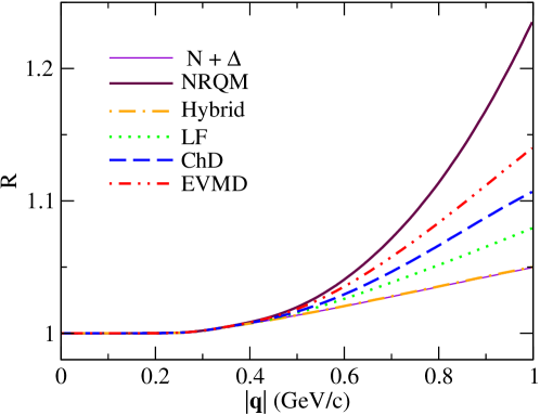
Figure 7: Resonance contribution to the Coulomb sum rule. The ratio $\mathcal{R}$ defined in Eq. (37) is evaluated including only the $\Delta$ (solid thin line) and including both $\Delta$ and Roper (thick lines) for the various models introduced above. Notice that the Roper contribution in the hybrid model is negligible and practically coincides with that of the $\Delta$ alone.

These findings imply that the resonances studied here should be accounted for when deriving a realistic Coulomb sum rule, especially when this is used to extract $NN$ correlations from experiment, at momentum transfers above 500 MeV$/c$. By the same token the contribution from other $N^{*}$ resonances (beyond the Roper) is also likely to be important and should be studied.

5 Parity-violating response functions

5.1 General formalism

Parity-violating effects due to weak interactions can be accessed in polarized inclusive electron scattering experiments by measuring the helicity asymmetry [34]

$${\mathcal{A}}=\left(\frac{d\sigma}{d\Omega^{\prime}dE^{\prime}}\right)^{(PV)}\Bigg{/}\left(\frac{d\sigma}{d\Omega^{\prime}dE^{\prime}}\right)^{(PC)}\,.$$ (38)

The PC cross section is given by Eq. (4) while the PV one, defined as the difference of the cross sections with opposite helicities of the initial electron, is expressed in terms of the corresponding PV response functions according to

$$\left(\frac{d\sigma}{d\Omega^{\prime}dE^{\prime}}\right)^{(PV)} \equiv \frac{1}{2}\left(\frac{d\sigma^{+}}{d\Omega^{\prime}dE^{\prime}}-\frac{d\sigma^{-}}{d\Omega^{\prime}dE^{\prime}}\right)$$ (39)

$$= \sigma_{\scriptscriptstyle{M}}\frac{1}{2EE^{\prime}\cos^{2}{\theta_{e}/2}}\mathcal{A}_{0}\widetilde{L}_{\mu\nu}\widetilde{W}^{\mu\nu}$$

$$= \sigma_{\scriptscriptstyle{M}}\mathcal{A}_{0}\left(v_{\scriptscriptstyle{L}}R^{\scriptscriptstyle{L}}_{\scriptscriptstyle{AV}}+v_{\scriptscriptstyle{T}}R^{\scriptscriptstyle{T}}_{\scriptscriptstyle{AV}}+v_{\scriptscriptstyle{T^{\prime}}}R^{\scriptscriptstyle{T^{\prime}}}_{\scriptscriptstyle{VA}}\right)\,,$$

where

$$\mathcal{A}_{0}=\frac{G_{\scriptscriptstyle{F}}|Q^{2}|}{2\sqrt{2}\pi\alpha}\,,$$ (40)

$G_{\scriptscriptstyle{F}}$ being the Fermi constant and

$$v_{\scriptscriptstyle{T^{\prime}}}=\sqrt{\frac{\tau}{\boldsymbol{\kappa}^{2}}+\tan^{2}{\frac{\theta_{e}}{2}}}\tan{\frac{\theta_{e}}{2}}\,.$$ (41)

The leptonic tensor is

$$\widetilde{L}_{\mu\nu}=a_{\scriptscriptstyle{A}}L_{\mu\nu}+a_{\scriptscriptstyle{V}}\left(-i\epsilon_{\mu\nu\alpha\beta}k^{\alpha}k^{{}^{\prime}\beta}\right)\,,$$ (42)

with $a_{\scriptscriptstyle{A}}=-1$ and $a_{\scriptscriptstyle{V}}=-(1-4\sin^{2}{\theta_{\scriptscriptstyle{W}}})$, $\theta_{\scriptscriptstyle{W}}$ being the weak angle of the standard electroweak theory. The following relations between the hadronic PV tensor $\widetilde{W}^{\mu\nu}$ and the response functions follow from Eq. (39)

$$R^{\scriptscriptstyle{L}}_{\scriptscriptstyle{AV}} \equiv a_{\scriptscriptstyle{A}}\widetilde{R}^{\scriptscriptstyle{L}}=a_{\scriptscriptstyle{A}}\widetilde{W}^{00}\,,$$ (43)

$$R^{\scriptscriptstyle{T}}_{\scriptscriptstyle{AV}} \equiv a_{\scriptscriptstyle{A}}\widetilde{R}^{\scriptscriptstyle{T}}=a_{\scriptscriptstyle{A}}\left(\widetilde{W}^{11}+\widetilde{W}^{22}\right)\,,$$ (44)

$$R^{\scriptscriptstyle{T^{\prime}}}_{\scriptscriptstyle{AV}} \equiv a_{\scriptscriptstyle{V}}\widetilde{R}^{\scriptscriptstyle{T^{\prime}}}=-i2a_{\scriptscriptstyle{V}}\widetilde{W}^{12}\,.$$ (45)

For $\widetilde{W}^{\mu\nu}$, Eqs. (8,9,10) hold if one replaces $f^{\mu\nu}$ by

$$\widetilde{f}^{\mu\nu}= -\widetilde{w}_{1}(\tau,\mu^{*})\left(g^{\mu\nu}+\frac{\kappa^{\mu}\kappa^{\nu}}{\tau}\right)+\widetilde{w}_{2}(\tau,\mu^{*})V^{\mu}V^{\nu}$$ (46)

$$-i\widetilde{w}_{3}(\tau,\mu^{*})\epsilon_{\mu\nu\alpha\beta}\kappa^{\alpha}V^{\beta}\,.$$

It is then straightforward to obtain the standard expressions for the PV response functions, namely

$$\widetilde{R}^{{\scriptscriptstyle{L}},{\scriptscriptstyle{T}},{\scriptscriptstyle{T^{\prime}}}}(|\mathbf{q}|,\omega)=\int^{\mu^{*}_{max}}_{\mu^{*}_{min}}d\mu^{*}G(\mu^{*})\widetilde{R}_{0}^{{\scriptscriptstyle{L}},{\scriptscriptstyle{T}},{\scriptscriptstyle{T^{\prime}}}}(|\mathbf{q}|,\omega,\mu^{*})$$ (47)

and

$$\widetilde{R}_{0}^{{\scriptscriptstyle{L}},{\scriptscriptstyle{T}},{\scriptscriptstyle{T^{\prime}}}}(|\mathbf{q}|,\omega,\mu^{*})=\frac{3{\mathcal{N}}}{4|\boldsymbol{\kappa}|m_{\scriptscriptstyle{N}}\eta_{\scriptscriptstyle{F}}^{3}}\xi_{\scriptscriptstyle{F}}\,\Theta(1-\psi^{2})(1-\psi^{2})\widetilde{U}^{{\scriptscriptstyle{L}},{\scriptscriptstyle{T}},{\scriptscriptstyle{T^{\prime}}}}(|\mathbf{q}|,\omega,\mu^{*})\,,$$ (48)

where

$$\widetilde{U}^{\scriptscriptstyle{L}} = \frac{\boldsymbol{\kappa}^{2}}{\tau}\left[(1+\tau\rho^{2})\widetilde{w}_{2}(\tau,\mu^{*})-\widetilde{w}_{1}(\tau,\mu^{*})+\widetilde{w}_{2}(\tau,\mu^{*}){\mathcal{D}}(\kappa,\mu^{*})\right]\,,$$ (49)

$$\widetilde{U}^{\scriptscriptstyle{T}} = 2\widetilde{w}_{1}(\tau,\mu^{*})+\widetilde{w}_{2}(\tau,\mu^{*}){\mathcal{D}}(\kappa,\mu^{*})\,,$$ (50)

$$\widetilde{U}^{\scriptscriptstyle{T^{\prime}}} = 2\sqrt{\tau(1+\tau\rho^{2})}\widetilde{w}_{3}(\tau,\mu^{*})\left[1+{\mathcal{D}}^{\prime}(\kappa,\mu^{*})\right]\,.$$ (51)

The function ${\mathcal{D}}(\kappa,\mu^{*})$ is defined in Eq. (18), while

$${\mathcal{D}}^{\prime}(\kappa,\mu^{*})=\frac{1}{|\boldsymbol{\kappa}|}\sqrt{\frac{\tau}{1+\tau\rho^{2}}}\left[1+\xi_{\scriptscriptstyle{F}}(1+\psi^{2})+\lambda\rho\right]-1\,.$$ (52)

As in the PC case, all of the dynamical information is carried by the functions $\widetilde{w}_{1,2,3}(\tau,\mu^{*})$.

5.2 Hadronic tensor and form factors

The PV $N-N^{*}(1440)$ hadronic tensor arises from the interference between the electromagnetic and the weak neutral currents

$$\widetilde{f}^{\mu\nu}=\frac{1}{2}\mu^{*}\mathrm{Tr}\left[\frac{(p\!\!\!\!\>/+m_{\scriptscriptstyle{N}})}{2m_{\scriptscriptstyle{N}}}\left(\gamma_{0}J_{em}^{\dagger\mu}\gamma_{0}\right)\frac{(p\!\!\!\!\>/^{\prime}+W)}{2W}J_{nc}^{\nu}\right]\,;$$ (53)

$J_{em}$ is given in Eq. (21) while $J_{nc}$ contains a vector and an axial-vector part. The vector current has the same structure as the electromagnetic one and the axial current is given in terms of axial and pseudoscalar form factors just as in the nucleon case:

$$J_{nc}^{\alpha}=J_{\scriptscriptstyle{V}}^{\alpha}+J_{\scriptscriptstyle{A}}^{\alpha}$$ (54)

with

$$J_{\scriptscriptstyle{V}}^{\alpha}=\bar{u}_{N^{*}}(p^{\prime})\left[\widetilde{F}_{1}(q^{2})\left(q\!\!\!\!\>/\,q^{\alpha}-q^{2}\gamma^{\alpha}\right)+i\widetilde{F}_{2}(q^{2})\sigma^{\alpha\beta}q_{\beta}\right]u(p)\,,$$ (55)

$$J_{\scriptscriptstyle{A}}^{\alpha}=\bar{u}_{N^{*}}(p^{\prime})\left[\widetilde{G}_{\scriptscriptstyle{A}}\gamma^{\alpha}\gamma_{5}+\widetilde{G}_{\scriptscriptstyle{P}}q^{\alpha}\gamma_{5}\right]u(p)\,.$$ (56)

It is convenient to introduce the weak form factors $\widetilde{G}_{\scriptscriptstyle{E,M}}$ related to $\widetilde{F}_{1,2}$ exactly as the electromagnetic form factors in Eqs. (24,25) and it is then possible to express $\widetilde{G}_{\scriptscriptstyle{E,M}}$ in terms of $G_{\scriptscriptstyle{E,M}}$. Following [35] one gets

$$2\widetilde{G}^{p(n)}_{\scriptscriptstyle{E,M}}=(1-4\sin^{2}{\theta_{\scriptscriptstyle{W}}})G^{p(n)}_{\scriptscriptstyle{E,M}}-G^{n(p)}_{\scriptscriptstyle{E,M}}\,.$$ (57)

In a similar way, $\widetilde{G}_{\scriptscriptstyle{A}}$ can be written as

$$2\widetilde{G}^{p(n)}_{\scriptscriptstyle{A}}=G^{p(n)}_{\scriptscriptstyle{A}}-G^{n(p)}_{\scriptscriptstyle{A}}=\pm G^{\scriptscriptstyle{V}}_{\scriptscriptstyle{A}}\,.$$ (58)

Lacking any experimental information or model calculations for the $N-N^{*}(1440)$ transition axial-vector form factor $G^{\scriptscriptstyle{V}}_{\scriptscriptstyle{A}}$, as in [28] we take

$$G^{\scriptscriptstyle{V}}_{\scriptscriptstyle{A}}(Q^{2})=2f_{\pi}\frac{\tilde{f}}{m_{\pi}}\left(1+\frac{|Q^{2}|}{M_{\scriptscriptstyle{A}}^{2}}\right)^{-2}\,,$$ (59)

where the value at $Q^{2}=0$ has been derived assuming pion pole dominance in the divergence of the axial current. Here, $f_{\pi}=92.4$ MeV is the pion decay constant [29] and $\tilde{f}=0.48$ is the $N^{*}\rightarrow N\,\pi$ coupling (see the Appendix). The dipole form for the $Q^{2}$ dependence with $M_{\scriptscriptstyle{A}}\approx 1$ GeV is inspired by the analogous behavior of the nucleon axial form factor. The pseudoscalar form factor $\widetilde{G}_{\scriptscriptstyle{P}}$ can, in principle, be related to $\widetilde{G}_{\scriptscriptstyle{A}}$ if one assumes partial conservation of the axial current (PCAC) [28]. However, since for PV electron scattering we require only the transverse projections of the axial-vector current, which do not include the pseudoscalar contributions, the latter are not needed in the present work. For purely weak interaction processes, and then only when mass terms must be retained, is it necessary to include such contributions (see, for example, [36]).

Finally, substituting the electromagnetic and neutral currents in Eq. (53) and comparing the result with the general form of $\widetilde{f}^{\mu\nu}$ in Eq. (46), one obtains

$$\widetilde{w}_{1} = \displaystyle\left[\tau+\frac{(\mu^{*}-1)^{2}}{4}\right]G_{\scriptscriptstyle{M}}\widetilde{G}_{\scriptscriptstyle{M}}\,,$$ (60)

$$\widetilde{w}_{2} = \displaystyle\frac{1}{\displaystyle 1+\frac{4\tau}{(\mu^{*}+1)^{2}}}\left[G_{\scriptscriptstyle{E}}\widetilde{G}_{\scriptscriptstyle{E}}+\frac{4\tau}{(\mu^{*}+1)^{2}}G_{\scriptscriptstyle{M}}\widetilde{G}_{\scriptscriptstyle{M}}\right]\,,$$ (61)

$$\widetilde{w}_{3} = \displaystyle G_{\scriptscriptstyle{M}}\widetilde{G}_{\scriptscriptstyle{A}}\,.$$ (62)

5.3 Results and discussion

In Fig. 8 we present the PV $N-N^{*}(1440)$ response functions together with those for the $N-\Delta$ [37, 25], at $|\mathbf{q}|=500$ and $1000$ MeV$/c$, and for ¹²C ($k_{\scriptscriptstyle{F}}=225$ MeV$/c$, $Z=N=6$) as in the PC case. We have used the helicity amplitudes from the five models displayed in Fig. 2. The Roper contribution to the transverse and axial responses is much smaller than in the case of the $\Delta$, so that the differences between the models do not appreciably change the results for the full response functions. In the case of $\widetilde{U}^{\scriptscriptstyle{T^{\prime}}}$, Eq. (59) has been used for $G^{\scriptscriptstyle{V}}_{\scriptscriptstyle{A}}$ in all cases. Different model calculations of these form factors will not change the situation appreciably, since the $q^{2}=0$ limit is not likely to be very different from the estimate based on PCAC, while the details of the $q^{2}$ dependence have little impact on the response functions, especially at low $|\mathbf{q}|$.

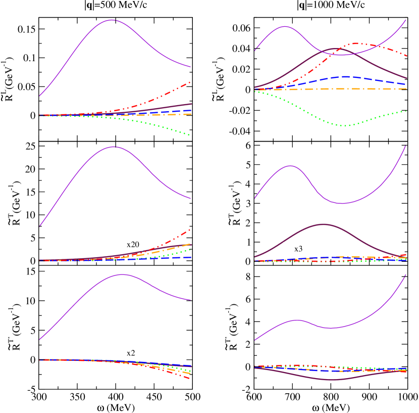
Figure 8: PV $N-N^{*}(1440)$ and $N-\Delta$ (thin solid lines) responses. In the case of the Roper, the helicity amplitudes of Fig. 2 have been used; the line styles are the same as in Figs. 3 and 5. Notice that in some of the plots, the $N-N^{*}(1440)$ responses have been multiplied by factor 20, 3 and 2.

The longitudinal response, in spite of its smallness, displays some interesting features. At $|\mathbf{q}|=500$ MeV$/c$, the results obtained with the NRQM, hybrid and ChD models is small while the LF and, particularly, EVMD approaches produce sizable (compared with the $\Delta$) responses of opposite signs. In order to understand the origin of such different behaviors we have calculated the $\tau\rightarrow 0$ limit of $\widetilde{U}^{\scriptscriptstyle{L}}$ in terms of the helicity amplitudes as in Eq. (31), obtaining

$$\widetilde{U}_{p}^{\scriptscriptstyle{L}}(\lambda\rightarrow|\boldsymbol{\kappa}|) = \left(\frac{m_{\scriptscriptstyle{N}}}{2\pi\alpha}\right)\bigg{[}8\boldsymbol{\kappa}^{2}\frac{\mu^{*2}}{\mu^{*2}-1}S_{1/2}^{p}(0)\widetilde{S}_{1/2}^{p}(0)$$ (63)

$$+ |\boldsymbol{\kappa}|\xi_{\scriptscriptstyle{F}}(1-\psi_{0}^{2})A_{1/2}^{p}(0)\widetilde{A}_{1/2}^{p}(0)\bigg{]}\,,$$

where

$$2\widetilde{A}_{1/2}^{p} = (1-4\sin^{2}{\theta_{\scriptscriptstyle{W}}})A_{1/2}^{p}-A_{1/2}^{n}$$ (64)

$$2\widetilde{S}_{1/2}^{p} = (1-4\sin^{2}{\theta_{\scriptscriptstyle{W}}})S_{1/2}^{p}-S_{1/2}^{n}\,.$$ (65)

The contribution arising from the neutrons ($\widetilde{U}_{n}^{\scriptscriptstyle{L}}$) is obtained by interchanging the labels $p$ and $n$ in the above equations. As we argued in Sec. 2.4, the factors in front of the helicity amplitudes are such that only the $S_{1/2}\widetilde{S}_{1/2}$ term matters. Since $(1-4\sin^{2}{\theta_{\scriptscriptstyle{W}}})\approx 0.092$, the term proportional to $S_{1/2}^{p2}(0)$ is disfavored with respect to the one proportional to $-S_{1/2}^{p}(0)S_{1/2}^{n}(0)$; $S_{1/2}^{n}(0)\neq 0$ only for LF and EVMD models (with different signs), as can be seen in Fig. (2). This shows how the nuclear PV response functions mix the information about the $N-N^{*}$ transitions on protons and neutrons in a non-trivial way.

In Figs. 9, 10 we show the asymmetry including the quasielastic contribution, the $\Delta$ and the $N^{*}(1440)$ for $|\mathbf{q}|=500$ and $1000$ MeV$/c$, respectively, and for forward (10^∘) and backward (170^∘) angles. In the case of the lower $|\mathbf{q}|$ the contribution of the $N^{*}(1440)$ to the asymmetry is negligible. Here, as well as in the case of the PC cross section previously discussed, the sizable contribution to $\tilde{R}^{L}$ is completely suppressed by $v_{L}$ (see the right panel).

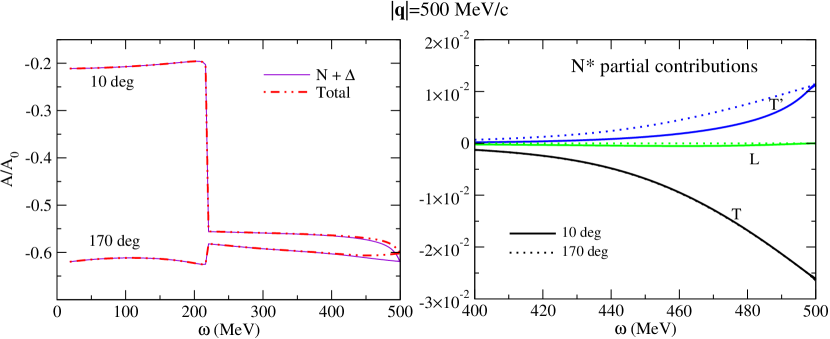
Figure 9: Left panel: the asymmetry in the $N+\Delta$ (solid) and $N+\Delta+N^{*}$ (dot-dashed) model for $|\mathbf{q}|=500$ MeV$/c$ at forward and backward angles; right panel: the separate contributions of the $N^{*}$ to the asymmetry in the $L$, $T$ and $T^{\prime}$ channels.

Hence the statement made in [37] interpreting the deviation from flatness of the asymmetry as a signal of the $N-\Delta$ axial response is not affected by the Roper resonance at least at low momentum transfer. On the other hand, at $|\mathbf{q}|=1000$ MeV$/c$, the Roper contribution changes the asymmetry above the quasielastic peak appreciably. Note that in this case the various models considered do not differ much from one other; only the NRQM does, and it is in fact one of the least favored by the data on the proton. Nevertheless, the striking effect predicted in [37], namely of an increase in magnitude of the asymmetry of about a factor three occurring at forward angles in passing from the QEP to the $\Delta$ peak domain, still persists.

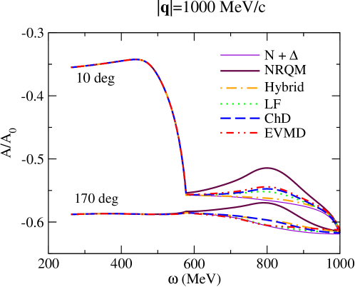
Figure 10: The same as the left panel of Fig. 9, but now for $|\mathbf{q}|=1000$ MeV$/c$. The contribution of the Roper is displayed for various models of the transition amplitudes.

6 Conclusions

We have studied the nuclear PC and PV response functions for the $N-N^{*}(1440)$ transition within the RFG framework. Empirical parameterizations and a selection of the model calculations available in the literature for the electromagnetic helicity amplitudes have been used as an input. The responses show some sensitivity to the various models. In particular, the non-relativistic quark model and the hybrid model with a large gluon component predict a quite different PC longitudinal response $R_{\scriptscriptstyle{L}}$. Also the $R_{\scriptscriptstyle{L}}$ associated with the Roper can be large compared with the contribution arising from the $\Delta$ near the light-cone. However, although in principle the study of the longitudinal response function in this region could provide valuable information about the nature of the Roper resonance, in practice this is hard to achieve because here the longitudinal response is much suppressed. On the other hand, given a longitudinal/transverse separation, the impact of the Roper on the Coulomb sum rule can be significant, as seen in Fig. 7.

Our results show that values of the momentum transfer around 500 MeV$/c$ are the most favorable for studies of $N-N^{*}(1440)$ transitions because here the Roper signal is already relatively large due to its considerable width, while heavier resonances are not likely to be too disruptive. A similar observation has been recently made in a study of photoproduction of the $N^{*}(1440)$ and vector mesons ($\rho$, $\omega$) [38].

In spite of the difficulties discussed in the paper with studying this elusive excitation of the nucleon, the interest in pursuing an in-medium investigation of the Roper resonance, as we have done here, relates in part to the role it plays as a breathing mode of the nucleon. It is the analog of the breathing mode of the nucleus (the isoscalar monopole mode) which carries information on the compressibility of nuclear matter. The same should occur at the nucleonic level, and hence a study of the nucleon’s compressibility, both in free space and embedded in the nuclear medium, may help in understanding the nature of hadronic matter including the problem of confinement.

It should be kept in mind that our treatment of nuclear effects is restricted to the inclusion of Fermi motion; hence it represents only a first step. More work is required to take into account polarization effects, meson exchange currents and in-medium renormalization in order to treat the second resonance region with the same level of sophistication achieved for the $\Delta$ and the quasielastic peaks.

Finally, it is worth pointing out that the contributions of the $N^{*}(1520)$ and $N^{*}(1535)$ to the nuclear responses should also be accounted for before drawing too specific conclusions on the role of the Roper. Also we have treated the $\Delta$ and the Roper as independent particles, but since both decay mainly into the $N\pi$ channel it is advisable to model non-resonant contributions and to estimate the importance of interference effects within a consistent framework. The spirit of the present exploratory study has been to determine whether or not such an ambitious program is warranted.

7 Acknowledgments

We thank J. A. Caballero, C. Maieron, M. Post and M. J. Vicente Vacas for useful discussions. This work has been supported in part by the Spanish DGICYT contract number BFM2000-1326 and in part (TWD) by funds provided by the U.S. Department of Energy under cooperative research agreement No. DE-DC02-94ER40818.

Appendix A The width of the Roper resonance

We express the total energy-dependent width of the $N^{*}(1440)$ as the sum of three contributions, $N\pi$, $\Delta\pi$ and $N(\pi\pi)^{I=0}_{s-wave}$ decay modes,

$$\Gamma(W)=\Gamma_{N\pi}(W)+\Gamma_{\Delta\pi}(W)+\Gamma_{N\pi\pi}(W)\,.$$ (66)

The more uncertain $N\rho$ channel [29] has been neglected. $\Gamma_{N\pi}$ exhibits a p-wave structure which, in the nonrelativistic limit, can be cast as [18]

$$\Gamma_{N\pi}(W)=\frac{3}{2\pi}\left(\frac{\tilde{f}}{m_{\pi}}\right)^{2}\frac{m_{\scriptscriptstyle{N}}}{W}|\mathbf{q}_{cm}|^{3}\,,$$ (67)

where $\mathbf{q}_{cm}$ is the pion 3-momentum in the resonance rest frame. The coupling $\tilde{f}=0.48$ is obtained assuming a total width of 350 MeV (at $W=m^{*}$) and an $N\pi$ branching ratio of 65% [29].

An accurate evaluation of the $N^{*}\rightarrow\Delta\pi$ width requires one to take into account the width of the $\Delta$ resonance. The fact that the $\Delta$ width is not small compared with the mass difference between the Roper and the $\Delta$ makes this correction advisable. The width is then expressed as [21]

$$\Gamma_{\Delta\pi}(W)=\frac{1}{3\pi^{2}}\left(\frac{g_{N^{*}\Delta\pi}}{m_{\pi}}\right)^{2}\int_{0}^{|\mathbf{p}|_{max}}d|\mathbf{p}|\,\frac{\mathbf{p}^{4}}{\sqrt{\mathbf{p}^{2}+m_{\pi}^{2}}}\left|D_{\Delta}(W_{\Delta})\right|^{2}\Gamma_{\Delta}(W_{\Delta})\,,$$ (68)

where $D_{\Delta}(W_{\Delta})$ is the $\Delta$ propagator

$$D_{\Delta}(W_{\Delta})=\frac{1}{W_{\Delta}-M_{\Delta}+\frac{1}{2}i\Gamma_{\Delta}(W_{\Delta})}\,,$$ (69)

$\Gamma_{\Delta}$ is the standard p-wave $\Delta\rightarrow N\pi$ partial decay width,

$$W_{\Delta}^{2}=W^{2}-2W(\sqrt{\mathbf{p}^{2}+m_{\pi}^{2}})+m_{\pi}^{2}\,,$$ (70)

and

$$\mathbf{p}_{max}^{2}=\left(\frac{W^{2}-m_{\scriptscriptstyle{N}}^{2}-2m_{\scriptscriptstyle{N}}m_{\pi}}{2W}\right)^{2}-m_{\pi}^{2}\,.$$ (71)

Using a branching ratio of 25% one obtains $g_{N^{*}\Delta\pi}=2.07$.

Finally, if we use the simplest possible Lagrangian for the $N^{*}\rightarrow N(\pi\pi)^{I=0}_{s-wave}$ channel as in [18], the decay width is given by

$$\Gamma_{N\pi\pi}(W)=3c^{2}\frac{1}{2^{5}\pi^{3}}\frac{m_{\scriptscriptstyle{N}}}{W^{2}}\int^{(W-m_{\scriptscriptstyle{N}})^{2}}_{4m_{\pi}^{2}}\frac{dx}{x}\lambda^{1/2}(W^{2},x,m_{\scriptscriptstyle{N}}^{2})\lambda^{1/2}(x,m_{\pi}^{2},m_{\pi}^{2})$$ (72)

with

$$\lambda(x,y,z)=x^{2}+y^{2}+z^{2}-2(xy+xz+yz)\,,$$ (73)

assuming a branching ratio of 7.5%, $c=2.3/m_{\pi}$.

References

- [1] S. Boffi, C. Giusti and F.D. Pacati, Phys. Rept. 226 (1993) 1.
- [2] J.E. Amaro et al., Phys. Rept. 368 (2002) 317, nucl-th/0204001.
- [3] T.W. Donnelly et al., Nucl. Phys. A541 (1992) 525.
- [4] A. Gil, J. Nieves and E. Oset, Nucl. Phys. A627 (1997) 543, nucl-th/9711009.
- [5] V.D. Burkert, (2002), hep-ph/0210321.
- [6] V.D. Burkert, AIP Conf. Proc. 603 (2001) 3, nucl-ex/0109004.
- [7] J. Lehr, M. Effenberger and U. Mosel, Nucl. Phys. A671 (2000) 503, nucl-th/9907091.
- [8] L.Y. Glozman and D.O. Riska, Phys. Rept. 268 (1996) 263, hep-ph/9505422.
- [9] Y.B. Dong et al., Phys. Rev. C60 (1999) 035203.
- [10] F. Cano and P. Gonzalez, Phys. Lett. B431 (1998) 270, nucl-th/9804071.
- [11] F. Cardarelli et al., Phys. Lett. B397 (1997) 13, nucl-th/9609047.
- [12] M.P. Mattis and M. Karliner, Phys. Rev. D31 (1985) 2833.
- [13] L.C. Biedenharn, Y. Dothan and M. Tarlini, Phys. Rev. D31 (1985) 649.
- [14] Z.p. Li, V. Burkert and Z.j. Li, Phys. Rev. D46 (1992) 70.
- [15] O. Krehl et al., Phys. Rev. C62 (2000) 025207, nucl-th/9911080.
- [16] P. Alberto et al., Phys. Lett. B523 (2001) 273, hep-ph/0103171.
- [17] C. Gerhardt, Z. Phys. C4 (1980) 311.
- [18] E. Oset and M.J. Vicente-Vacas, Nucl. Phys. A446 (1985) 584.
- [19] L. Alvarez-Ruso, E. Oset and E. Hernandez, Nucl. Phys. A633 (1998) 519, nucl-th/9706046.
- [20] H.P. Morsch et al., Phys. Rev. Lett. 69 (1992) 1336.
- [21] S. Hirenzaki, P. Fernandez de Cordoba and E. Oset, Phys. Rev. C53 (1996) 277, nucl-th/9511036.
- [22] W.M. Alberico et al., Phys. Rev. C38 (1988) 109.
- [23] T.W. Donnelly and J.D. Walecka, Ann. Rev. Nucl. Sci. 25 (1975) 329.
- [24] J.E. Amaro et al., Nucl. Phys. A657 (1999) 161, nucl-th/9905035.
- [25] L. Alvarez-Ruso et al., Phys. Lett. B497 (2001) 214, nucl-th/0007036.
- [26] R.C.E. Devenish, T.S. Eisenschitz and J.G. Korner, Phys. Rev. D14 (1976) 3063.
- [27] H.J. Weber, Phys. Rev. C41 (1990) 2783.
- [28] L. Alvarez-Ruso, S.K. Singh and M.J. Vicente Vacas, Phys. Rev. C57 (1998) 2693, nucl-th/9712058.
- [29] Particle Data Group, D.E. Groom et al., Eur. Phys. J. C15 (2000) 1.
- [30] M.B. Barbaro et al., Nucl. Phys. A643 (1998) 137, nucl-th/9804054.
- [31] C. Maieron, T.W. Donnelly and I. Sick, Phys. Rev. C65 (2002) 025502, nucl-th/0109032.
- [32] T.W. Donnelly and I. Sick, Phys. Rev. C60 (1999) 065502, nucl-th/9905060.
- [33] T.W. Donnelly, E.L. Kronenberg and J.W. Van Orden, Nucl. Phys. A494 (1989) 365.
- [34] J.D. Walecka, Nucl. Phys. A285 (1977) 349.
- [35] M.J. Musolf et al., Phys. Rept. 239 (1994) 1.
- [36] T.W. Donnelly and R.D. Peccei, Phys. Rept. 50 (1979) 1.
- [37] P. Amore et al., Nucl. Phys. A690 (2001) 509, nucl-th/0007072.
- [38] M. Soyeur, Nucl. Phys. A671 (2000) 532, nucl-th/0003047.