A non-perturbative approach to halo breakup

Abstract

The theory of weakly bound cluster breakup, like halo nucleus breakup, needs an accurate treatment of the transitions from bound to continuum states induced by the nuclear and Coulomb potentials. When the transition probability is not very small, a non-perturbative framework might be necessary. Nuclear excitation dominates at small impact parameters whereas the Coulomb potential being long range acts over a larger impact parameter interval. In this article, we propose an effective breakup amplitude which meets a number of requirements necessary for an accurate quantitative description of the breakup reaction mechanism. Furthermore our treatment gives some insight on the interplay between time dependent perturbation theory and sudden approximation and it allows to include the nuclear and Coulomb potentials to all orders within an eikonal-like framework.

PACS number(s):25.70.Hi, 21.10Gv,25.60Ge,25.70Mn,27.20+n

Key-words Nuclear breakup, Coulomb breakup, high order effects, halo nuclei.

1 Introduction

Break up of halo nuclei is a stimulating field for reaction mechanism studies where accurate reaction theories are needed in order to extract spectroscopic information from experimental data. These theories should treat together very different excitations induced by electromagnetic and nuclear fields to all orders. Recently a number of interesting papers have appeared in which the problem of nuclear and Coulomb breakup is solved numerically either by a direct solution of the single particle Schrödinger equation [1]-[7], or by DWBA type of approaches [8] or by an approximate treatment of the coupled equations in the continuum [9]. Of these papers only Refs.[2, 6, 8, 9] have treated at the same time the nuclear and Coulomb processes. Still one needs analytical models to complete the understanding of the mechanisms involved and test approximations which could help reduce the computational difficulties and help extending the models to more structured clusters. Various analytical solutions of the Coulomb breakup problem exist where the problem of the higher order effects has been studied [1]. In this paper, we propose an effective amplitude for breakup to all orders in the interactions which reveals the interplay between sudden and time dependent perturbation theory.

Nuclear breakup is a short time process, several observables of which are reasonably well described by the sudden approximation [7, 10]. In the case of the electromagnetic field, things are more complicated since the Coulomb potential is a long range field. Hence, in Section 2 of this paper we present the theoretical framework for the simultaneous treatment of nuclear and Coulomb interactions. The effective amplitude we propose is introduced in Section 3 where we show also how one can establish the accuracy of different approximations based on the relative behavior of two parameters. The last part of this article is dedicated to the discussion of some calculations and to their comparison with experimental data.

2 Eikonal theory of nuclear and Coulomb breakup

In a recent paper [11] we presented a full description of the treatment of the scattering equation for a projectile which decays by single neutron breakup due to its interaction with the target. There it was shown that within the semiclassical approach for the projectile-target relative motion, the amplitude for a transition from a nucleon bound state $\psi_{i}$ in the projectile to a final continuum state $\psi_{f}$ is given by

$$g_{fi}={1\over i\hbar}\int_{-\infty}^{\infty}dt<\psi_{f}(t)|V({\bf r})|\psi_{i}(t)>,$$ (1)

where $V$ is the interaction responsible for the neutron transition to the continuum.

For light targets the recoil effect due to the projectile-target Coulomb potential is rather small and the interaction responsible for the reaction is mainly the neutron-target nuclear potential. In the case of heavy targets the dominant reaction mechanism is Coulomb breakup. The Coulomb force does not act directly on the neutron but it affects it only indirectly by causing the recoil of the core. Therefore the neutron is subject to an effective force which gives rise to an effective Coulomb dipole potential $V_{\rm eff}({\bf r,R}(t))$ (cf. Eq. (23) of the Appendix). ${\bf R}(t)={\bf\hat{x}}d+{\bf\hat{z}}vt$ is the core-target relative distance and ${\bf r}$ is the neutron-core coordinate. In ref.[11] it was shown that the combined effect of the nuclear and Coulomb interactions to all orders can be taken into account by using the potential ${V}=V_{\rm nt}+V_{\rm eff}$ sum of the neutron-target optical potential and the effective Coulomb dipole potential. If for the neutron final continuum wave function we take a distorted wave of the eikonal-type, then the amplitude in the projectile reference frame becomes :

$$g_{fi}\left(\mathbf{k,}{\bf d}\right)=\frac{1}{i\hbar}\int\!\!d^{3}{\bf r}\int dt{\rm e}^{-i{\bf k\cdot r}+i\omega t-i\chi_{\rm eik}({\bf r},t)}{V}\left({\bf r},t\right)\phi_{i}\left(\mathbf{r}\right)$$ (2)

where $\phi_{i}$ is the time independent part of the neutron initial wave function and $i\equiv(l,m)$ stands for the angular momentum quantum numbers, $\omega=\left({{\varepsilon^{\prime}_{f}}}-\varepsilon_{0}\right)/\hbar$ and $\varepsilon_{0}$ is the neutron initial bound state energy while ${{\varepsilon^{\prime}_{f}}}$ is the final neutron-core continuum energy. ${\bf k}\equiv(k_{x},k_{y},k_{z})$ is a real vector and the eikonal phase shift is simply

$$\chi_{\rm eik}({\bf r},t)=\frac{1}{\hbar v}\int_{t}^{\infty}V({\bf r},t^{\prime})dt^{\prime}$$ (3)

where $v$ is the relative motion velocity at the distance of closest approach. Integrating by parts Eq. (2) leads to the equivalent expression for the breakup amplitude :

$$g_{fi}\left(\mathbf{k,}{\bf d}\right)=-\int\!\!dt{\rm e}^{i\omega t}\frac{d}{dt}\int\!\!d^{3}{\bf r}{\rm e}^{-i{\bf k}\cdot{\bf r}-i\chi_{\rm eik}({\bf r},t)}\phi_{i}\left(\mathbf{r}\right).$$ (4)

Eq. (2) is appropriate to calculate the coincidence cross section $A_{p}\to(A_{p}-1)+n$. Finally the differential probability with respect to the neutron energy and angles can be written as

$${d^{3}P_{bu}(d)\over d{{\varepsilon^{\prime}_{f}}}d\Omega^{\prime}}={1\over 8\pi^{3}}{mk\over\hbar^{2}}{1\over 2l_{i}+1}\Sigma_{m_{i}}|g_{fi}\left(\mathbf{k,}{\bf d}\right)|^{2}.$$

where $g_{fi}$ is given by Eq. (2) and we have averaged over the neutron initial state.

Eq. (2) can be in principle an useful alternative to full numerical solutions of the Schrödinger equation. In fact it contains all partial waves in the final eikonal-like wave function and still the full time dependence, while the numerical solutions so far available are often restricted to the first few partial waves in the development of the final continuum wave function. Finally the differential breakup cross section is given by an integration over core-target impact parameters

$${d^{2}\sigma\over{d{{\varepsilon^{\prime}_{f}}}d\Omega^{\prime}}}=C^{2}S\int_{0}^{\infty}d{\bf d}{d^{2}P_{bu}(d)\over d{{\varepsilon^{\prime}_{f}}d\Omega^{\prime}}}P_{ct}(d),$$ (5)

and $C^{2}S$ is the spectroscopic factor for the initial single particle orbital. The effects associated with the core-target interaction have been included by multiplying the breakup probability by $P_{ct}(d)=|S_{ct}|^{2}$ [12] the probability for the core to be left in its ground state, defined in terms of a core-target S-matrix function of $d$, the core-target distance of closest approach. A simple parameterization is $P_{ct}(d)=\exp(-(\ln 2)\exp[(R_{s}-d)/a])$, where the strong absorption radius $R_{s}\approx 1.4(A_{p}^{1/3}+A_{t}^{1/3})$ fm is defined as the distance of closest approach for a trajectory that is 50% absorbed from the elastic channel and $a=0.6$ fm is a diffusness parameter.

There have been already in the literature a large number of papers dealing with the problem of higher order effects in halo breakup and therefore it is important to understand the relation between our model and other approaches. By using a first order time dependent amplitude in Eq. (1) we are assuming that breakup is a one step process in which the neutron is emitted in the continuum by a single interaction with the nuclear target potential and by core recoil. The nuclear and Coulomb potential are seen as final state interactions which distort the simple plane wave which otherwise would be the final continuum state of the neutron. Because of the long tail of the halo wave function the overlap between $\psi({\bf r})$ and the potential $V({\bf r})$ is large and the potential needs to be treated to all orders. This approach is fully consistent with the usual treatment of higher order effect by the electromagnetic field [1].

3 Approximation scheme : BBM 1 and BBM 2 amplitudes

Since it is already well established that the nuclear potential needs to be considered to all orders for weakly bound projectiles, in [11] we studied numerically only the limits of pure nuclear breakup to all orders, of Coulomb breakup to first order and of the coupling between Coulomb to first order and nuclear to all orders. On the other hand we argued that the question of if and when the Coulomb potential needs to be treated to all orders was still under investigation. Here we report on new calculations that we have recently performed by using Eq. (2) to treat in detail Coulomb higher order effects.

Expanding the time dependent perturbation theory amplitude Eq. (2) in powers of the eikonal phase shift Eq.(3)

$$g_{\rm CN}=g_{\rm CN}^{1}+g_{\rm CN}^{2}+g_{\rm CN}^{3}+\dots$$ (6)

we get a series of partial amplitudes. From here on we avoid the indices _fi to simplify the notation. Treating separately the nuclear and Coulomb potential Eq. (6) reduces to

$$g^{\rm pert}_{\rm C}=g_{\rm C}^{\rm pert\,1}+g_{\rm C}^{\rm pert\,2}+g_{\rm C}^{\rm pert\,3}+\dots$$ (7)

$$g^{\rm pert}_{\rm N}=g_{\rm N}^{\rm pert\,1}+g_{\rm N}^{\rm pert\,2}+g_{\rm N}^{\rm pert\,3}+\dots$$ (8)

On the other hand if we make the sudden approximation $\omega=0$ then the analogous amplitudes are

$$g^{\rm sudd}_{\rm C}=g_{\rm C}^{\rm sudd\,1}+g_{\rm C}^{\rm sudd\,2}+g_{\rm C}^{\rm sudd\,3}+\dots$$ (9)

$$g^{\rm sudd}_{\rm N}=g_{\rm N}^{\rm sudd\,1}+g_{\rm N}^{\rm sudd\,2}+g_{\rm N}^{\rm sudd\,3}+\dots$$ (10)

In Eq. (9) each term corresponds to the n^th term of the standard eikonal approximation to the theory of Coulomb excitations [13], while in Eq. (7) $g_{\rm C}^{\rm pert\,1}$ is the standard first order perturbation theory. Also we know already that the sudden approximation gives an accurate framework for the nuclear breakup, then $g_{\rm N}^{\rm pert\,i}-g_{\rm N}^{\rm sudd\,i}\approx 0$ for each order, such that $g^{\rm sudd}_{\rm N}\approx g^{\rm pert}_{\rm N}$.

Eq. (9) is much easier to calculate than Eq. (7), however it has the very well known drawback that the first order term leads to a logarithmic divergence when used in the integral over impact parameters Eq. (5). Under the hypothesis that higher order terms are accurately calculated by the sudden approximation, we propose the use of an effective amplitude defined as:

$$g_{\rm C}^{\rm BBM\,1}\equiv\left(g_{\rm C}^{\rm sudd}-g_{\rm C}^{\rm sudd\,1}\right)+g_{\rm C}^{\rm pert\,1}$$ (11)

We want to treat the nuclear process at the same level of approximation, hence, it is straightforward to show that the generalization of $g_{\rm C}^{\rm BBM\,1}$ which includes also the nuclear potential to all orders and the coupling between the nuclear and the Coulomb effective potential is simply

$$g_{\rm CN}^{\rm BBM\,1} \approx g_{\rm C}^{\rm pert\,1}+g_{\rm N}^{\rm pert\,1}+\left(g_{\rm CN}^{\rm sudd}-g_{\rm C}^{\rm sudd\,1}-g_{\rm N}^{\rm sudd\,1}\right)$$ (12)

$$\equiv g_{\rm C}^{\rm pert\,1}+\left(g_{\rm CN}^{\rm sudd}-g_{\rm C}^{\rm sudd\,1}\right).$$

In the above equation the choice to treat terms higher than the first order within the sudden approximation might seem somewhat arbitrary. Then, we define another amplitude, BBM 2, for which we keep the time dependence in both first and second order terms, sudden approximation being used starting from the third order term :

$$g_{\rm CN}^{\rm BBM\,2} \equiv g_{\rm C}^{\rm pert\,1}+g_{\rm C}^{\rm pert\,2}+\left(g_{\rm CN}^{\rm sudd}-g_{\rm C}^{\rm sudd\,1}-g_{\rm C}^{\rm sudd\,2}\right)$$ (13)

$$+ \left(g_{\rm C}^{\rm\,pert\,1}-g_{\rm C}^{\rm sudd\,1}\right)g_{\rm N}^{\rm sudd\,1}$$

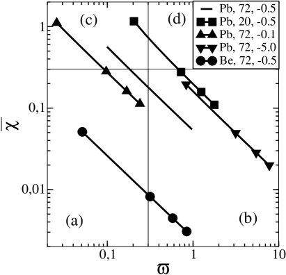
Figure 1: Perturbation parameter $\bar{\chi}$ versus adiabaticity parameter $\varpi$ for impact parameters between $R_{s}$ and 110 fm and for the reaction ¹¹Be+${\rm Target}$. We vary the target (Pb, Be), the energy of the beam (72, 20 A.MeV) and the binding energy of the neutron (-0.1, -0.5, -5 MeV). Four regions where different theories should be valid are indicated: (a) sudden first order, (b) first order time dependent, (c) sudden to all order, (d) time dependent to all orders.

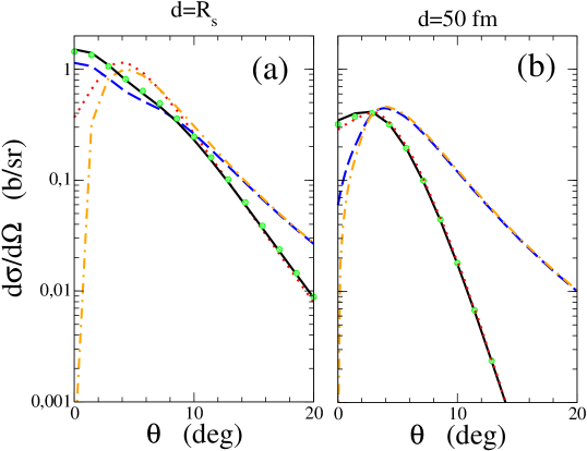
Figure 2: Neutron angular distributions for the reaction ¹¹Be+¹⁹⁷Au at 41 A.MeV at $d=R_{s}$ and 50 fm. Solid line is the result of $g_{\rm C}^{\rm BBM\,1}$ compared to $g_{\rm CN}^{\rm BBM\,2}$ calculated without nuclear potential (big dots). The dotted line is the first order perturbation theory calculation, dashed line is the sudden to all orders while dot-dashed line is the sudden to first order result.

This approximation scheme solves several problems encountered in the treatment of halo breakup: the already mentioned logarithmic divergence in the impact parameter integral due to the the first order sudden approximation, the requirement to treat the Coulomb and the nuclear field at the same level of approximation and to all orders for small impact parameters and the need to use time dependent perturbation theory for large impact parameters where the Coulomb field is effective for a long time. A quantitative justification of our approximation scheme is given by the discussion of Fig. (1) in the next section. On the other hand the discussion of Fig. (2) where the results obtained with BBM1 and BBM2 are compared will clarify the treatment of higher order terms by the eikonal approximation.

4 Time dependent framework and its sudden approximation

In this section we give some explicit expressions for the amplitudes discussed in Sec.(3). We start by considering the Coulomb term only and in particular the first order approximation for it, thus $\exp(-i\chi_{\rm eff})=1$ and $V_{\rm nt}=0$, but the $\omega t$ term is kept in Eq. (4) (this is the standard first order time dependent perturbation theory amplitude)

$$g^{\rm pert\,1}_{\rm C}\left({\bf k},{\bf d};lm\right) = Q\left(\varpi K_{1}\left(\varpi\right)\frac{d}{dk_{x}}+i\varpi K_{0}\left(\varpi\right)\frac{d}{dk_{z}}\right)\tilde{\phi}_{lm}\left(\mathbf{k}\right).$$ (14)

Here $Q=2{\beta}_{1}Z_{P}Z_{T}e^{2}/\hbar vd$ is the classical Coulomb momentum transfer to the neutron due to the core recoil. $K_{1}$ and $K_{0}$ are the usual modified Bessel functions. The adiabaticity parameter $\varpi={{\varepsilon}^{\prime}_{f}-\varepsilon_{0}\over\hbar v}d$ represents the ratio of the collision time ($d/v$) over the nuclear interaction time. If the reaction mechanism is such that $\varpi$ is small, then the nuclear interaction time is greater than the collision time and the sudden approximation becomes accurate.

Then we consider the sudden approximation in which $\omega=0$ and Eq. (2) can be calculated with the nuclear and Coulomb potentials to all orders giving

$$g^{\rm sudd}_{\rm CN}\left({\bf k},{\bf d};lm\right)=\int d^{2}\mathbf{r}_{\perp}{\rm e}^{-i\mathbf{k}_{\perp}\cdot\mathbf{r}_{\perp}}\left({\rm e}^{-i(\chi_{\rm nt}\left({\bf r}_{\perp}\right)+\chi_{\rm eff}\left({\bf r}_{\perp}\right))}-1\right)\tilde{\phi}_{lm}\left(\mathbf{r}_{\perp},k_{z}\right),$$ (15)

where

$$\chi_{\rm eff}\left({\bf r}_{\perp}\right) = \int_{-\infty}^{\infty}dt~{}~{}V_{\rm eff}({\bf r,R}(t))=Qx$$ (16)

and $V_{\rm eff}$ is given by Eq. (23). However as we mentioned above, in a first step we study only the effects of the Coulomb potential. Thus we call $g_{\rm C}^{\rm sudd}$ the amplitude obtained from Eq. (15), by setting the nuclear potential equal to zero. Then the Coulomb amplitude in the sudden approximation to all orders can be written as

$$g^{\rm sudd}_{\rm C}\left({\bf k},{\bf d};lm\right) = \int d^{2}\mathbf{r}_{\perp}e^{-i\mathbf{k}_{\perp}\mathbf{.r}_{\perp}}\left(e{{}^{-iQx}}-1\right)\tilde{\phi}_{lm}\left(\mathbf{r}_{\perp},k_{z}\right)$$ (17)

$$= \tilde{\phi}_{lm}\left(k_{x}+Q,k_{y},k_{z}\right)-\tilde{\phi}_{lm}\left(k_{x},k_{y},k_{z}\right)$$

In the limit of very small $Q$ Eq. (17) gives

$$g^{\rm sudd\,1}_{\rm C}\left({\bf k},{\bf d};lm\right)\approx Q\frac{d}{dk_{x}}\tilde{\phi}_{lm}\left(k_{x},k_{y},k_{z}\right)$$ (18)

which is the sudden approximation restricted to first order and it agrees with the perturbation formula in the sudden limit, because $\varpi K_{1}\left(\varpi\right)=1$ and $\varpi K_{0}\left(\varpi\right)=0$ when $\varpi=0$. If the initial state wave function is approximated by its asymptotic form which is an Hankel function

$$\phi_{lm}({\bf r})=-i^{l}C_{i}\gamma_{0}h_{l}^{(1)}(i\gamma_{0}r)Y_{lm}(\theta,\phi),\,\,\,\gamma_{0}r>>1,$$ (19)

where $C_{i}$ is the asymptotic normalization constant and $\gamma_{0}=\sqrt{-2m\varepsilon_{0}}/\hbar$, then the general form of the initial state momentum distribution is given by the Fourier transform of Eq.(19) :

$$\widetilde{\phi}_{lm}({\bf k})=4\pi C_{i}\frac{(k/\gamma_{0})^{l}}{({\bf k}^{2}+\gamma_{0}^{2})}Y_{lm}(\hat{{\bf k}})$$ (20)

For the 2s_1/2 halo state of ${}^{11}Be$ it reads

$$\widetilde{\phi}_{00}(k)=2\sqrt{\pi}C_{i}{1\over({\bf k}^{2}+\gamma_{0}^{2})}=2\sqrt{\pi}C_{i}{1\over K^{2}}$$ (21)

Where we have put $K^{2}={\bf k}^{2}+\gamma_{0}^{2}$. By defining the dimensionless strength parameter $\bar{\chi}={Q/K}$ and using Eq. (21), the sudden to all orders amplitude calculated explicitly up to second order in $\bar{\chi}$ reads

$$g^{\rm sudd}_{\rm C}\left({\bf k},{\bf d};00\right) = -{2\sqrt{\pi}C_{i}\over K^{2}}\left[{2k_{x}\over K}\bar{\chi}+\left(1-{4k_{x}^{2}\over K^{2}}\right)\bar{\chi}^{2}+...\right]$$ (22)

In Appendix A, Eqs.(29) and (30), we give the expansion of the amplitude up to second order in the full time dependent approach. Eq. (22), can also be obtained from those equations in the limit $\varpi\to 0$. The strength parameter $\bar{\chi}$ represent the ratio of the classical Coulomb momentum transfer $Q$ over the momentum $K$ which is an average of the neutron final and initial momenta. If $\bar{\chi}$ is small, then a first order theory is accurate. From Eq. (22) one sees that if $k_{x}=0$, which happens for example for scattering at zero degrees, the amplitude gets contribution starting from the second order term. Thus the higher order terms are important for a proper description of the forward angle neutrons.

The transition from the perturbative to the non-perturbative but all orders regime can be studied by plotting the strength parameter $\bar{\chi}$ vs the adiabaticity parameter $\varpi$ using the impact parameter as a variable. We show in Fig. (1) the results obtained for various combinations of incident beam energy and neutron separation energy and different targets as indicated in the figure. The case of low incident energy clearly needs an exact treatment of Coulomb breakup because at all impact parameters both the strength parameter $\bar{\chi}$ as well as the adiabaticity parameter $\varpi$ get values close to one. In the other cases instead, there is always one of the two limits which works well. For small separation energies (0.1MeV) $\varpi$ is very small and one can use the sudden approximation to all orders. On the other hand for large separation energies (5MeV) $\bar{\chi}$ is always small and the first order perturbation theory is accurate enough. In the cases we are discussing in this paper there is a smooth transition from one regime to the other and the transition occurs for impact parameters such that $\bar{\chi}\approx\varpi$ which is satisfied in our case for $d=d_{\rm crit}=\sqrt{Z_{\rm eff}/\sqrt{2}\gamma_{0}|\epsilon_{0}|}$. This discussion and our formulation of the sudden approximation are very close in spirit to the work of Typel and Baur [17] and to ref.[18].

Table 1: For several reactions discussed in this paper, we give the associated strong absorption radius $R_{s}$ and the critical impact parameter $d_{\rm crit}$. The maximum value of the impact parameter is always $d=120$ fm.

	Target	$E_{\rm inc}$ (A.MeV)	$R_{s}$ (fm)	$d_{\rm crit}$ (fm)
11Be	Be	41	6.0	4.4
	Ti	41	8.2	10.2
	Au	41	11.3	19.4
	Pb	72	11.4	19.8
19C	Pb	67	12.0	18.4

5 Results

We discuss now the behavior of $g_{\rm C}^{\rm BBM\,1}$. An interesting observable which has been measured in a few experiments [23, 26] is the exclusive neutron angular distribution. The data of [23] were taken at 41 A.MeV therefore it would be interesting to check if our model works reasonably well at such low energy. We show in Fig. (2) (a) and (b) angular distributions for the Coulomb breakup alone calculated for the reaction ¹¹Be+¹⁹⁷Au at 41 A.MeV at two impact parameters $d=R_{s}$, and $d=50$ fm. The solid line is the result obtained from $g_{\rm C}^{\rm BBM\,1}$ which is compared to the result from $g_{\rm CN}^{\rm BBM\,2}$ without nuclear interaction (big dots), the dotted line is the first order perturbation theory calculation, dashed line is the sudden to all orders while dot-dashed line is the sudden to first order result. We see that at small impact parameters the sudden to first order and the sudden to all orders give coincident results, starting from an angle of about 10 deg. At $d=50$ fm already the sudden to all orders and the sudden to first order give the same results at all angles. Thus it appears that higher order effects are important only at small neutron angles and at small impact parameters. Also in these situations the $g_{\rm C}^{\rm BBM\,1}$ amplitude Eq. (11) reduces to the first order perturbation theory amplitude Eq. (14). Eq. (11) can be considered correct only if the treatment of higher order terms by the sudden approximation, is accurate. This is indeed shown in Fig. (2) by the results obtained with the effective formula corrected to second order $g_{\rm CN}^{\rm BBM\,2}$ (big dots) calculated without nuclear potential.

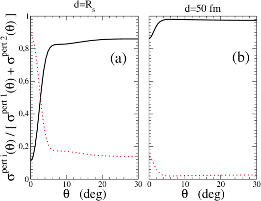
Figure 3: Same reaction as Fig. (2), the lines are ratios of differential cross sections as a function of neutron angle. The solid and dotted lines are the ratios of the first and second order time dependent perturbation theory cross sections respectively divided by their sum.

At angles smaller than 10 deg and small impact parameters the all orders calculation is different from the first order calculation. This is due to higher orders terms in the Coulomb field. Fig. (3) clarify this point: we represent the contribution of the first and the second order calculation normalized by their sum. It is clear that second order is very important at small neutron angles for small impact parameters whereas at large impact parameters, its effects are negligible.

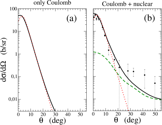
Figure 4: Same reaction as Fig. (2) with the full d-integration. In both figures the dotted line is first order perturbation theory. On the left hand side figure, the solid line is the calculation with the effective amplitude including only the Coulomb potential, while on the right hand side the solid line includes both nuclear and Coulomb effects and the dashed line is the nuclear breakup alone. Data are from [23].

The angular distributions integrated over impact parameters are shown in Fig. (4) (a) and (b). The result with the $g_{\rm C}^{\rm BBM\,1}$ amplitude in (a) is shown by the full line while the result with the Coulomb first order amplitude is the dotted line. In the case of pure Coulomb breakup, the first order amplitude is accurate enough down to 10 degrees, where higher order terms in the Coulomb field flatten the angular distribution. Such behavior seems indeed to be present in the experimental data which are shown on the right hand side figure together with the nuclear contribution. Our results explain why first order perturbation theory has been so successful in earlier studies of Coulomb breakup and they provide also a further justification of our previous approach [11]. Note that for lighter targets the data do show a peak slightly shifted from zero degrees, thus reflecting the less important effect of higher order contributions [23]. In Fig. (4) (b) we give instead by the solid line the results from $g_{\rm CN}^{\rm BBM\,1}$ including Coulomb and nuclear potential. For completeness we give also by the dashed line the nuclear contribution alone and the experimental data from [23].

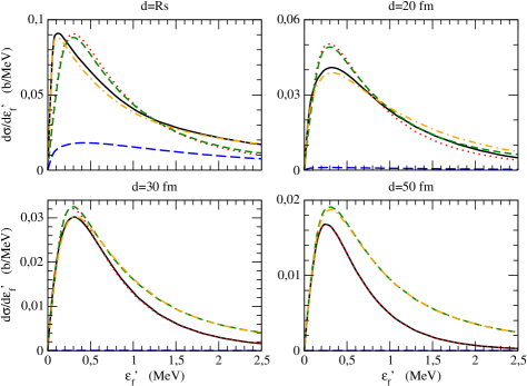
Figure 5: Neutron-target energy distributions from ¹¹Be+²⁰⁸Pb at 72 A.MeV for several impact parameters. Solid line is the result of $g_{\rm CN}^{\rm BBM\,1}$, the dotted line is the first order perturbation theory calculation, dashed line is the first order sudden calculation, the long dashed is the nuclear sudden to all orders and dot-dashed line is the Coulomb plus nuclear sudden to all orders result.

We present now results relative to energy distributions obtained for the reaction ¹¹Be(²⁰⁸Pb,²⁰⁸Pb)¹⁰Be+$n$ at $E_{\rm inc}$=72 A.MeV [24]. In Fig. (5) we give the results of the calculations obtained by the amplitude $g_{\rm CN}^{\rm BBM\,1}$, including both nuclear and Coulomb potential, Eq. (12), by the solid line. The sudden all-order amplitude (dot-dashed line) Eq. (15), the first order perturbation theory (dotted curve) Eq. (14) and the sudden first order (short dashed) Eq. (18) for an impact parameter corresponding to the strong absorption radius $d=R_{s}$ and to $d$=20, 30 and 50 fm. The long dashed line gives only the nuclear contribution. At small impact parameters the two first order calculations, sudden and time dependent perturbation theory are very close, thus showing that the sudden approximation is valid at small impact parameters and therefore suggesting that Eq. (17) would be accurate at small impact parameters to calculate the all orders amplitude. On the other hand we see that starting from $d=30$ fm a new regime applies in which the two sudden calculations, to all orders or to first order give the same results. Then we conclude again that at high impact parameters the higher order effects can be neglected and first order perturbation theory applies.

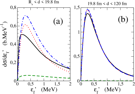
Figure 6: Same as Fig. (5) with integration over impact parameters smaller and larger than the critical value (cf. Table 1). The solid line is the $g_{\rm CN}^{\rm BBM\,1}$ result, dotted is Coulomb first order perturbation theory, dashed line is nuclear sudden to all orders and dotted-dash line is the previous result from [11].

The main results of our new calculations are shown in Fig. (6) (a) and (b) by the solid thick line. The effective formula $g^{\rm BBM\,1}_{\rm CN}$ has been integrated in the impact parameter range smaller and larger than $d_{crit}=19.8$ fm respectively. These calculations indicate that for $R_{s}<d<19.8$ fm the results obtained with $g^{\rm BBM\,1}_{\rm CN}$, solid line, are smaller than those obtained with first order perturbation theory $g^{\rm pert\,1}_{\rm C}$, thus showing higher order terms need to be considered. Since from the angular distributions shown in the previous figures one can see that the effect of the higher order terms in Coulomb breakup alone is rather small, we suggest that the strong depletion shown by the peak of the energy distributions including Coulomb and nuclear breakup, comes mainly from the destructive interference effect already discussed in [11]. On the other hand for $d>19.8$ fm we find that higher order effects are negligible since using the effective formula or perturbation theory gives very little difference. We have checked that for

$d>30$ fm perturbation theory agrees exactly with the effective formula. Then we can conclude that at large $d$ perturbation theory is valid. It is then reasonable to think that experimental data for neutron breakup could be analyzed by first order perturbation theory provided one could extract the contribution from impact parameters somewhat larger than $d_{crit}$. As we mentioned before, it is important to notice that the amplitude defined as $g^{\rm BBM\,1}_{\rm C}$, valid at all core-target impact parameters does not give rise to any divergences in the final integral over impact parameters. This is because the first order sudden term $g^{\rm sudd\,1}_{\rm C}$ which contains the divergence is removed and substituted by the first order time dependent perturbation theory term $g^{\rm pert\,1}_{\rm C}$ which does not diverge. The dashed line gives the nuclear contribution alone and the dot-dashed line is the result of our previous method [11], recalculated using relativistic kinematics for consistency with all other results of this paper.

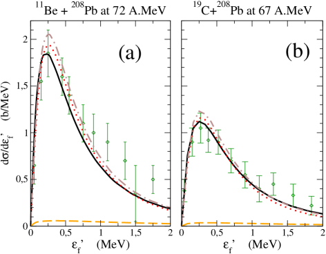
Figure 7: Comparison between calculations and experimental results for the reactions: (a) ¹¹Be+²⁰⁸Pb at 72 A.MeV and (b) ¹⁹C+²⁰⁸Pb at 67 A.MeV (right). The solid line is the $g^{\rm BBM\,1}_{\rm CN}$ result, dotted is Coulomb first order perturbation theory, dashed line is nuclear sudden to all orders and dot-dashed line is previous results from [11]. The spectroscopic factor used are $C^{2}S=0.77$ for ¹¹Be and $C^{2}S=0.65$ for ¹⁹C. Data are from [24, 25].

Finally the results of the full impact parameter integration are shown in Fig. (7) which gives the neutron final energy spectrum with respect to the core for breakup of ¹¹Be and ¹⁹C on ²⁰⁸Pb at 72 A.MeV and 67 A.MeV respectively. Experimental data are from [24, 25]. Notations are as in Fig. (6). In the case of ¹¹Be the theoretical calculations have been multiplied by the known spectroscopic factor $C^{2}S=0.77$, while for ¹⁹C we have used $C^{2}S=0.65$ and a neutron separation energy for the 2s state of 0.5 MeV. As expected, and already shown by other authors the effects of higher order terms are to reduce the peak cross section [1]. Analysis of the type presented in this section have been used to extract spectroscopic factors.

6 Conclusions

In this work we have presented an approximation scheme which allows calculating Coulomb and nuclear breakup and their coupling to all orders. It appears that higher order terms can give some effect only for heavy targets, at low core-target impact parameters and small neutron angles, and their effect is still noticeable after integrating over impact parameters. We have shown that higher order effects are accurately calculated by the sudden approximation. The neutron angular distribution observable is well reproduced by the time dependent perturbation theory of Coulomb breakup. Once again we would like to stress the usefulness of measuring neutron angular distributions following breakup, as one of the best observables to clarify reaction mechanisms and to test theoretical models.

The neutron-core relative energy spectrum after breakup shows a depletion of the peak value when higher order effects are included. It appears that this is mainly due to the destructive interference between nuclear and Coulomb breakup. Our conclusions are in agreement with recent numerical solutions of the breakup problem [1, 2, 8] and with new experimental data [26]. In particular as higher order effects in the Coulomb potential are important only for small impact parameters ($d<d_{\rm crit}$), in order to extract spectroscopic factors without any ambiguities, it appears very well suited to compare Coulomb first order perturbation theory with data containing contributions from $d>d_{\rm crit}$ only [26].

One neutron halo breakup is a simple reaction mechanism for which our approximation scheme allows to treat higher order terms in the Coulomb and the nuclear fields at the same time, including their couplings. This approximation scheme leads to simple expressions which can be generalized to proton breakup, where one needs to include the particle-target Coulomb potential and its quadrupole component.

Aknowledgments

We wish to thank Stefan Typel for discussions and comments and for communicating his results previuos to publication.

Appendix A Eikonal perturbation theory for Coulomb breakup

We give here some explicit formulae for the eikonal perturbation theory in the case of an electromagnetic excitation. The Coulomb field from a target nucleus can act both on the core and on the halo nucleus. Here we are only interested in the part that acts on their relative position and cause the breakup. For this reason, we subtract the part that acts on the position of the center of mass and we obtain [19] :

$$V_{\rm eff}=Z_{T}e^{2}\left(\frac{Z_{h}}{|{\bf R}+\beta_{2}{\bf r}|}+\frac{Z_{C}}{|{\bf R}-\beta_{1}{\bf r}|}-\frac{Z_{C}+Z_{h}}{|{\bf R}|}\right)$$ (23)

where charges and masses are: core ($A_{C}$,$Z_{C}$), halo ($A_{h}$,$Z_{h}$), target ($A_{T}$,$Z_{T}$). We used also two ratios : $\beta_{1}=A_{h}/A_{P}$ and $\beta_{2}=A_{c}/A_{P}$, with $A_{P}=A_{C}+A_{h}$. We develop this interaction in series and we take the case of a zero charge halo thus getting the dipole field

$$V_{\rm eff}({\bf r},t) = f(t)x+g(t)z$$ (24)

where

$$f(t)=\frac{Z_{\rm eff}d}{\big{(}d^{2}+(vt)^{2}\big{)}^{3/2}}\hskip 28.45274pt{\rm and}\hskip 28.45274ptg(t)=\frac{Z_{\rm eff}vt}{\big{(}d^{2}+(vt)^{2}\big{)}^{3/2}}.$$

and $Z_{\rm eff}=\beta_{1}Z_{P}Z_{T}e^{2}$. According to the eikonal formalism, the phase shift is expressed in the simple form :

$$\chi_{\rm eff}({\bf r},t)=\int_{t}^{\infty}V_{\rm eff}({\bf r},t^{\prime})dt^{\prime} = F(t)x+G(t)z$$ (25)

with

$$F(t) = {1\over\hbar}\int_{t}^{\infty}f(t^{\prime})dt^{\prime}={Q\over 2}\left(1-\frac{s}{\sqrt{1+s^{2}}}\right)$$

$$G(t) = {1\over\hbar}\int_{t}^{\infty}g(t^{\prime})dt^{\prime}={Q\over 2}\frac{1}{\sqrt{1+s^{2}}}$$ (26)

where $s=vt/d$ and $Q=2Z_{\rm eff}/(\hbar vd)$.

Introducing Eq. (25) into Eq. (4) leads to

$$g^{\rm pert}_{\rm C}({\bf k},{\bf d};lm) = -\int\!\!dt\,{\rm e}^{i{\omega}t}\frac{d}{dt}\tilde{\phi}_{lm}({\bf k}_{t})$$ (27)

where ${\bf k}_{t}=\big{(}k_{x}+F(t),k_{y},k_{z}+G(t)\big{)}$. Using Eq. (21) the breakup amplitude from an initial s-state becomes

$$g^{\rm pert}_{\rm C}({\bf k},{\bf d};00)=4C_{i}\sqrt{\pi}\int dt\,{\rm e}^{i\omega t}\frac{f(t)[k_{x}+F(t)]+g(t)[k_{z}+G(t)]}{\left([k_{x}+F(t)]^{2}+{k_{y}}^{2}+[k_{z}+G(t)]^{2}+\gamma_{0}^{2}\right)^{2}}.$$ (28)

We obtain the eikonal perturbation theory from an expansion in powers of the phase shift. Due to the simple form of the phase shift $\chi_{\rm eff}=Qx$, we expand Eq. (28) with respect to the small quantities $F(t)k_{x}/K^{2}$ and $G(t)k_{z}/K^{2}$ which are proportional to the parameter $\bar{\chi}=Q/K$ used in Eq. (22), and neglect terms of order $F(t)^{2}$ and $G(t)^{2}$. Thus the first order term reads :

$$g^{\rm pert\,1}_{\rm C}({\bf k},{\bf d};00) = -\sqrt{\pi}C_{i}Q\frac{\varpi}{K^{4}}\Big{(}2k_{x}K_{1}(\varpi)+2ik_{z}K_{0}(\varpi)\Big{)}$$ (29)

where one sees that the adiabaticity parameter $\varpi$ appears naturally. The second order amplitude is

$$g^{\rm pert\,2}_{\rm C}({\bf k},{\bf d};00) = -{\sqrt{\pi}\over 2}C_{i}Q^{2}\frac{\varpi}{K^{6}}\Big{(}\big{(}K^{2}-4{k_{x}}^{2}\big{)}K_{1}(\varpi)-4ik_{x}k_{z}K_{0}(\varpi)$$ (30)

$$-i\pi({k_{z}}^{2}+2k_{x}k_{z}-{k_{x}}^{2}){\rm e}^{-\varpi}\Big{)}$$

The sudden approximation of these amplitudes are simply deduced as the limit $\varpi\rightarrow 0$.

In order to make a link with previous work [1] by other authors, we calculate explicitly the probability momentum distribution in the sudden approximation as:

$$\frac{dP^{s}({\bf d})}{dk}=\frac{1}{8\pi^{3}}\int d\Omega^{\prime}{k}^{2}|g^{\rm sudd}_{\rm C}({\bf k},{\bf d})|^{2}$$ (31)

Then, we find for the first order and second order terms in the dipole field

$$\frac{dP_{1}^{s}({\bf d})}{dk} = \frac{1}{8\pi^{3}}\int d\Omega^{\prime}{k}^{2}|g^{\rm sudd\,1}({\bf k},{\bf d})|^{2}=\frac{16y^{2}}{3\pi\gamma_{0}}\frac{x^{4}}{(1+x^{2})^{4}}$$ (32)

$$\frac{dP_{22}^{s}({\bf d})}{dk} = \frac{1}{8\pi^{3}}\int d\Omega^{\prime}{k}^{2}|g^{\rm sudd\,2}|^{2}=\frac{4y^{4}}{15\pi\gamma_{0}}\frac{x^{2}(15-10x^{2}+23x^{4})}{(1+x^{2})^{6}}$$ (33)

$$\frac{dP_{13}^{s}({\bf d})}{dk} = \frac{1}{8\pi^{3}}\int d\Omega^{\prime}{k}^{2}g^{\rm sudd\,1}g^{\rm sudd\,3}=-\frac{32y^{4}}{15\pi\gamma_{0}}\frac{x^{4}(5-x^{2})}{(1+x^{2})^{6}}$$ (34)

$$\frac{dP_{2}^{s}({\bf d})}{dk} = \frac{dP_{22}^{s}({\bf d})}{dk}+2\frac{dP_{13}^{s}({\bf d})}{dk}=\frac{4y^{4}}{15\pi\gamma_{0}}\frac{x^{2}(15-90x^{2}+39x^{4})}{(1+x^{2})^{6}}$$ (35)

with $x=k/\gamma_{0}$, $y=Q^{(D)}/\gamma_{0}$ and we used the asymptotic normalization constant $C_{i}^{2}=2\gamma_{0}$ of authors [1].

Our first order result Eq. (32) is identical with the equivalent term Eq. (2.6) of ref.[1]. The second order dipole-dipole term of this work Eq. (33) is different from Eq. (2.8) of [1]. The difference is due to the fact that in [1] the exact neutron-core scattering wave function

$$\phi_{f}({\bf k})={{\rm e}^{i{\bf k\cdot r}}}-{1\over{\gamma_{0}-ik}}{e^{ikr}\over r}.$$ (36)

was used, while in this paper the plane wave approximation has been applied, consistently with our hypothesis that the neutron-core final state interaction can be neglected (cf. Sec. 2 of [11]). We have checked that using Eq. (36) we would get the same result as in [1] but also that the difference with Eq. (33) is negligible. To show this point we give in Fig. (8) the sudden first order Coulomb breakup probability Eq.(32) after momentum integration as a function of the core-target impact parameter $d$ (solid line) and the second order dipole-dipole term Eq. (33) calculated according to Eq. (2) (dashed line) and with the final plane wave function substituted by Eq. (36) (short dashed line). It is clear that second order terms are rather small compared to the first order term, but also that the use of final plane waves is justified.

Appendix B Fourier Transforms for the Coulomb potential

$$\int dt\,{\rm e}^{i\omega t}f(t) = Q\varpi K_{1}(\varpi)$$ (37)

$$\int dt\,{\rm e}^{i\omega t}g(t) = iQ\varpi K_{0}(\varpi)$$ (38)

$$\int dt\,{\rm e}^{i\omega t}f(t)F(t) = {Q^{2}\over 4}\left(2\varpi K_{1}(\varpi)-i\frac{\pi}{2}\varpi{\rm e}^{-\varpi}\right)$$ (39)

$$\int dt\,{\rm e}^{i\omega t}g(t)G(t) = {Q^{2}\over 4}i\frac{\pi}{2}\varpi{\rm e}^{-\varpi}$$ (40)

$$\int dt\,{\rm e}^{i\omega t}f(t)G(t) = {Q^{2}\over 4}\frac{\pi}{2}(1+\varpi){\rm e}^{-\varpi}$$ (41)

$$\int dt\,{\rm e}^{i\omega t}g(t)F(t) = {Q^{2}\over 4}\left(2i\varpi K_{0}(\varpi)+\frac{\pi}{2}(-1+\varpi){\rm e}^{-\varpi}\right)$$ (42)

Figure 8: Comparison between the sudden first order Coulomb breakup probability Eq. (32) after momentum integration, as a function of the core-target impact parameter (dashed line) and the second order dipole-dipole term calculated according to Eqs. (2) and (33) (solid line) and with the final plane wave function substituted by Eq. (36) (dotted line).

References

- [1] S. Typel and G. Baur, Phys. Rev. C 64 (2001) 024601.
- [2] S. Typel and R. Shyam, Phys. Rev. C 64 (2001) 024605.
- [3] H. Esbensen, G. Bertsch and C.A. Bertulani, Nucl. Phys. A581 (1995) 107.
- [4] T. Kido, K. Yabana and Y. Suzuki, Phys. Rev. C 53 (1996) 2296.
- [5] V. S. Melezhik and D. Baye, Phys. Rev. C 59 (1999) 3232.
- [6] M. Fallot, J. A. Scarpaci, D. Lacroix, Ph. Chomaz and J. Margueron, Nucl. Phys. A700 (2002) 70.
- [7] H. Esbensen, and G. F. Bertsch, Phys. Rev. C 64 (2001) 014608; Nucl. Phys. A706 (2002) 383.
- [8] R. Chatterjee and R. Shyam, Phys. Rev. C 66 (2002) 061601.
- [9] F. M. Nunes and I. J. Thompson, Phys. Rev. C 59, (1999) 2652 and references therein.
- [10] A. Bonaccorso and G. F. Bertsch, Phys. Rev. C 63 (2001) 044604.
- [11] J.Margueron, A.Bonaccorso and D.M. Brink, Nucl. Phys. A703 (2002) 105 and references therein.
- [12] A. Bonaccorso, Phys. Rev. C 60 (1999) 054604 and references therein.
- [13] K. Alder and A. Winther, electromagnetic excitation (North-Holland, Amsterdam, 1975).
- [14] S. Typel and G. Baur, Phys. Rev. C 49 (1994) 379.
- [15] S. Typel and G. Baur, Phys. Rev. C 50 (1994) 2104.
- [16] S. Typel and G. Baur, Nucl. Phys. A573 (1994) 486.
- [17] S. Typel and G. Baur, Phys. Lett. B 356 (1995) 186.
- [18] Y.Tokimoto et al., Phys. Rev. C 63 (2001) 35801.
- [19] H.Esbensen, International school of heavy ion physics, Erice 11-20 May 1997, Ed R.A.Broglia and P.G.Hansen, World Scientific.
- [20] A. Bonaccorso and D. M. Brink, Phys. Rev. C 57 (1998) R22.
- [21] A. Bonaccorso and D. M. Brink, Phys. Rev. C 58 (1998) 2864.
- [22] A. Winther and K. Adler, Nucl. Phys. A319 (1979) 518.
- [23] R. Anne et al., Nucl. Phys. A575 (1994) 125.
- [24] T. Nakamura, Phys. Lett. B 331 (1994) 296.
- [25] T. Nakamura et al., Phys. Rev. Lett. 83 (1999) 1112.
- [26] T. Nakamura, in Proc. of the 4th Italy-Japan Symposium on Perspectives in Heavy Ion Physics, edited by K. Yoshida, S. Kubono, I. Tanihata, C. Signorini, (World Scientific, 2003), p. 25, and to be published.