Axial exchange currents and the spin content of the nucleon

D. Barquilla-Cano¹, A. J. Buchmann² and E. Hernández¹

Abstract

In a chiral quark model where chiral symmetry is introduced via a non-linear $\sigma$ model, we evaluate the axial couplings $g_{A}(0)$, $g_{A}^{8}(0)$ and $g_{A}^{0}(0)$ related to the spin structure of the nucleon. Our calculation includes one-body and two-body axial current and pion absorption operators, which satisfy the Partial Conservation of Axial Current (PCAC) condition. While $g_{A}(0)$ is dominated by the one-body axial current we find significant corrections due to two-body axial exchange currents in $g_{A}^{8}(0)$ and $g_{A}^{0}(0)$. Interestingly, the axial current associated with gluon exchange reduces $g_{A}^{8}(0)$ from 1 to 0.6. Our analysis shows that the so-called “proton spin crisis” can be resolved in a constituent quark model in which PCAC is satisfied. Furthermore, we use the PCAC constraint in order to determine the couplings of the $\eta$ and $\eta^{\prime}$ mesons to nucleons.

I Introduction

In a recent work [1] we have evaluated the axial form factors of the nucleon, $g_{A}$, $g_{P}^{non-pole}$ and $g_{T}$ in the context of a chiral constituent quark model. Chiral symmetry was introduced via a linear $\sigma$-model with pions and $\sigma$-meson degrees of freedom. The model is consistent with PCAC, up to some order in the nonrelativistic expansion of the axial quark operators. The PCAC constraint for the non-pole part of the axial current reads

$$[H,A^{non-pole,0}({\bf q})]-{\bf q}\cdot{\bf A}^{non-pole}({\bf q})=i\ \sqrt{2}\ f_{\pi}\ M^{\pi}({\bf q}),$$ (1)

where $H$ is the Hamiltonian of the three-quark system, including the center of mass motion, $q$$q$ $q$$q$  is the three-momentum transfer of the weak gauge boson, $A^{non-pole,\,\mu}\ (\mu=0,1,2,3)$ stands for the non-pole part of the axial current operator, $M^{\pi}$ is the pion absorption operator, and $f_{\pi}=92.4$ MeV is the empirical pion decay constant. Eq.(1) plays a similar role in constraining the form of the axial currents as the continuity equation for the electromagnetic current.

One of the main consequences of the PCAC relation for the axial current is that axial coupling of the constituent quarks, $g_{Aq}$, is not equal to unity. Instead, it is related to the pion-quark coupling constant, $g_{\pi q}$, via a Goldberger-Treiman relation. The second important consequence of the PCAC constraint is the necessity to include axial exchange currents into the quark model. The presence of two-body potentials in $H$ should be accompanied by two-body axial exchange currents and pion absorption operators if PCAC as formulated in Eq.(1) is to hold. The results of Ref. [1] show that the isovector axial coupling $g_{A}(0)$ of the nucleon is dominated by the one-body axial current. Gluon, pion, and scalar axial exchange currents, although they are individually quite large, add to an overall correction of less than $2\%$.

In the present paper we are interested in the two remaining axial nucleon couplings, namely the flavor octet isosinglet coupling $g_{A}^{8}(0)$ and its flavor singlet counterpart $g_{A}^{0}(0)$ related to the spin content of the nucleon. The spin fractions $\Delta q$ carried by the quarks of flavor $q$ are axial current matrix elements and can be evaluated in a constituent quark model. In the naive nonrelativistic quark model, which uses only one-body axial currents, one obtains $\Delta u=4/3$, $\Delta d=-1/3$ and $\Delta s=0$ and from them $g_{A}(0)=5/3$ and $g_{A}^{8}(0)=g_{A}^{0}(0)=1$. On the other hand, the experimental numbers are: $\Delta u=0.84\pm 0.02$, $\Delta d=-0.42\pm 0.02$, and $\Delta s=-0.09\pm 0.02$ [3] leading to $g_{A}(0)=1.26\pm 0.04$, $g_{A}^{8}(0)=0.60\pm 0.08$ and $g_{A}^{8}(0)=0.33\pm 0.06$.

This marked disagreement between theory and experiment has often been interpreted as a severe shortcoming of the constituent quark model (“spin crisis”). Here, we show that once the PCAC violating and commonly used approximations: (i) axial charge of the constituent quarks $g_{Aq}$ is equal to unity i.e., the same as for QCD quarks, (ii) neglect of two-body axial exchange currents, are removed [1], the calculated spin fractions are in good agreement with the experimental numbers.

The paper is organized as follows. In sect. II we review the relation between the axial current matrix elements and the spin fraction carried by the quarks as determined in deep inelastic lepton-nucleon scattering and octet baryon decays. Sect. III, reviews the non-linear $\sigma$-model of Manohar and Georgi, which is the basis of the chiral quark model used in sect. IV. The axial current operators are listed in sect. V, and our results for the nucleon spin structure are presented in sect. VI. There we also calculate the $\eta NN$ and $\eta^{\prime}NN$ coupling constants. A summary of our results is presented in sect. VII.

II Spin structure of the nucleon

In naive nonrelativistic constituent quark models, in which the three constituent quarks are in relative S-wave states, the nucleon spin is accounted for by the sum of the constituent quark spins. Since the late 1980’s we know from deep inelastic scattering experiments that only a small fraction of the proton spin is carried by the spin of the QCD (or current) quarks, and that there is a nonzero contribution to the nucleon spin arising from strange quark-antiquark pairs in the Dirac sea [2]. Recent experiments conclude that approximately $1/3$ of the spin of the nucleon is carried by QCD quarks [3]. Calling $\Delta q$ the fraction of the proton spin carried by quarks of flavor $q$, we have from Ref. [3]

$$\Delta u=\hskip 9.95863pt0.84\pm 0.02,\hskip 14.22636pt\Delta d=-0.42\pm 0.02,\hskip 14.22636pt\Delta s=-0.09\pm 0.02.$$ (2)

In a parton model description of the nucleon, the spin fractions of the total nucleon spin carried by the individual quark flavors are given as

$$\Delta q=\int_{0}^{1}dx\,\big{(}\,q_{+}(x)+\bar{q}_{+}(x)-q_{-}(x)-\bar{q}_{-}(x)\,\big{)}.$$ (3)

Here, $q_{\pm}(x)$ is the probability of finding in the nucleon a QCD quark of flavor $q$ with momentum fraction $x$ of the total nucleon momentum having its helicity parallel (+) or antiparallel (-) to the proton helicity. The quark momentum distribution functions $q_{\pm}(x)$ can be further decomposed as

$$q_{\pm}(x)=q^{val}_{\pm}(x)+q^{sea}_{\pm}(x),$$ (4)

where $q^{val}_{\pm}(x)$ ($q^{sea}_{\pm}(x)$) is the contribution of the QCD valence (sea) quarks; $\bar{q}_{\pm}(x)$ stands for the antiquark distribution function in the sea.

In deep inelastic lepton-proton scattering one is measuring the spin-dependent structure function $g_{1}^{p}(x,Q^{2})$ of the proton at high momentum transfers $Q^{2}$. The integral of this function $\Gamma_{1}^{p}=\int_{0}^{1}g_{1}^{p}(x,Q^{2})\ dx$ is given in the scaling limit by the parton model result  [4]

$$\Gamma_{1}^{p}=\frac{1}{2}\sum_{q}e_{q}^{2}\Delta q=\frac{4}{18}\Delta u+\frac{1}{18}\Delta d+\frac{1}{18}\Delta s$$ (5)

where $e_{q}$ is the quark charge of flavor q. The spin fractions can be expressed as axial vector current matrix elements

$$\langle\,p,s|\bar{q}\gamma_{\mu}\gamma_{5}q|p,s\rangle=\Delta q\,s_{\mu},$$ (6)

where $s_{\mu}$ is the spin vector.

Additional information on the spin fractions can be extracted from the weak semileptonic decay of octet baryons. From neutron $\beta$-decay one can extract the combination $g_{A}^{3}(0)=\Delta u-\Delta d$ which is nothing but the nucleon axial coupling constant $g_{A}(0)$. Also, from SU(3) flavor symmetry and experimentally known hyperon $\beta$-decays one obtains the spin fraction combination $g_{A}^{8}(0)=\Delta u+\Delta d-2\Delta s$. The two constants $g_{A}(0)$ and $g_{A}^{8}(0)$ govern all octet baryon $\beta$-decays in the flavor symmetry limit. The combined DIS and hyperon $\beta$-decay data give values for each $\Delta q$ as quoted above. While the use of SU(3) symmetry is not without controversy and has been sometimes severely critizied [5], some authors think that SU(3) symmetry breaking effects are small, of the order of 10% [6].

If the Dirac sea were SU(3) flavor symmetric, $g_{A}^{8}(0)$ would have the interpretation as the fraction of the proton spin carried by valence QCD quarks, whereas the total fraction of the proton spin carried by all QCD quarks is given by the quantity $g_{A}^{0}(0)=\Delta u+\Delta d+\Delta s$. Using the numbers [3] given above one obtains $g_{A}^{0}(0)=0.33\pm 0.06$, definitely smaller than 1, which is the expectation according to the naive nonrelativistic quark model. This is the origin of the so called “spin crisis”. The experimental result may change somewhat. From the use of the flavor tagging technique at the HERMES experiment it would be possible to obtain the spin fractions directly from deep inelastic scattering experiments without relying on the SU(3) flavor symmetry assumption. Preliminary results from the experiment show that $\Delta s>0$ in disagreement with the previous determination [7]. This latter result has been critizied on the account that it would take $g_{A}^{8}(0)$ out of any reasonable bounds [8].

Before we calculate the axial nucleon couplings we will review the SU(3) extended version of the non-linear $\sigma$-model, which is appropriate for the evaluation of $g_{A}^{8}(0)$ and $g_{A}^{0}(0)$.

III The non-linear $\sigma$ model

Let us start with the effective Lagrangian for the non-linear $\sigma$ model, which lends support to the notion of constituent quarks interacting via gluon and pseudoscalar boson exchange [9]. The effective Lagrangian is given by

$${\cal L}=\overline{\Psi}i\gamma^{\mu}(D_{\mu}+{\cal V}_{\mu})\Psi-M\overline{\Psi}\Psi+g_{Aq}\overline{\Psi}\gamma^{\mu}\gamma_{5}{\cal A}_{\mu}\Psi+\frac{f^{2}_{\pi}}{4}\ tr\left(\partial^{\mu}\Sigma^{\dagger}\partial_{\mu}\Sigma\right)-\frac{1}{2}\ tr\left(F_{\mu\nu}\,F^{\mu\nu}\right).$$ (7)

Here, $\Psi=(u,\,d,\,s)$ is the quark field and $M=m_{q}{\bf 1}$ is the quark mass matrix prior to any explicit SU(3) breaking. Furthermore, $D_{\mu}$ is the color SU(3)_C covariant derivative

$$D_{\mu}=\partial_{\mu}+i\,g\,G_{\mu},\qquad G_{\mu}=\frac{1}{2}\,\lambda_{j}^{c}\cdot G^{c}_{j,\mu},$$ (8)

where $G_{\mu}$ is the gluon field and the $\lambda_{j}^{c}$ are the color SU(3)_C Gell-Mann matrices. $F_{\mu\nu}$ is the gluon field strength tensor

$$F_{\mu\nu}=\partial_{\mu}\,G_{\nu}-\partial_{\nu}\,G_{\mu}+i\,g\,[G_{\mu},G_{\nu}].$$ (9)

The fields ${\cal V}_{\mu}$ and ${\cal A}_{\mu}$ appearing in Eq.(7) are given in terms of the matrix field $\xi$ derived from an octet of pseudoscalar boson fields $\Phi$$\Phi$ $\Phi$$\Phi$ 

$${\cal V}_{\mu}=\frac{1}{2}(\xi\partial_{\mu}\xi^{\dagger}+\xi^{\dagger}\partial_{\mu}\xi),\qquad{\cal A}_{\mu}=\frac{i}{2}(\xi\partial_{\mu}\xi^{\dagger}-\xi^{\dagger}\partial_{\mu}\xi).$$ (10)

The pseudo-scalar bosons $\Phi$$\Phi$ $\Phi$$\Phi$  are the Goldstone bosons (GB) associated with the spontaneous breaking of the $SU(3)_{V}\times SU(3)_{A}$ chiral symmetry. Following Ref. [9] we describe their dynamics in terms of a $3\times 3$ matrix field $\Sigma$ given by

$$\Sigma=e^{i\hbox{$\lambda$}\hbox to0.0pt{\hss\hbox{$\lambda$}\hskip 0.27995pt}\hbox to0.0pt{\hss\lower 0.12053pt\hbox{\hbox{$\lambda$}\hbox to0.0pt{\hss\hbox{$\lambda$}\hskip 0.27995pt}}}\cdot\hbox{$\Phi$}\hbox to0.0pt{\hss\hbox{$\Phi$}\hskip 0.27995pt}\hbox to0.0pt{\hss\lower 0.12053pt\hbox{\hbox{$\Phi$}\hbox to0.0pt{\hss\hbox{$\Phi$}\hskip 0.27995pt}}}/F}=\xi^{2}$$ (11)

where $\lambda$$\lambda$ $\lambda$$\lambda$  is a vector whose components $\lambda_{j}$ are the eight Gell-Mann matrices of SU(3) flavor symmetry, and $\Phi$$\Phi$ $\Phi$$\Phi$  stands for the eight GB fields $\Phi_{j}$, $j=1\cdots 8$. Here, $i=1,2,3$ stands for the isotriplet $\pi$, $i=4,\cdots 7$ for the two doublets of $K$, and $i=8$ for the $\eta$. With this normalization $F$ is the GB decay constant. Working in lowest order as we shall do

$$F=f_{\pi}=92.4\ {\rm MeV}.$$ (12)

The matrix field

$$\xi=e^{i\hbox{$\lambda$}\hbox to0.0pt{\hss\hbox{$\lambda$}\hskip 0.27995pt}\hbox to0.0pt{\hss\lower 0.12053pt\hbox{\hbox{$\lambda$}\hbox to0.0pt{\hss\hbox{$\lambda$}\hskip 0.27995pt}}}\cdot\hbox{$\Phi$}\hbox to0.0pt{\hss\hbox{$\Phi$}\hskip 0.27995pt}\hbox to0.0pt{\hss\lower 0.12053pt\hbox{\hbox{$\Phi$}\hbox to0.0pt{\hss\hbox{$\Phi$}\hskip 0.27995pt}}}/2f_{\pi}}$$ (13)

transforms under $SU(3)_{V}\times SU(3)_{A}$ as

$$\xi\stackrel{{\scriptstyle\stackrel{{\scriptstyle SU(3)_{V}}}{{}}}}{{\longrightarrow}}V\xi V^{\dagger}\qquad\xi\stackrel{{\scriptstyle\stackrel{{\scriptstyle SU(3)_{A}}}{{}}}}{{\longrightarrow}}A^{\dagger}\xi U^{\dagger}=U\xi A^{\dagger}$$ (14)

where $V=\exp(-i\hbox{$\lambda$}\hbox to0.0pt{\hss\hbox{$\lambda$}\hskip 0.39993pt}\hbox to0.0pt{\hss\lower 0.17218pt\hbox{\hbox{$\lambda$}\hbox to0.0pt{\hss\hbox{$\lambda$}\hskip 0.39993pt}}}\cdot\hbox{$\alpha$}\hbox to0.0pt{\hss\hbox{$\alpha$}\hskip 0.39993pt}\hbox to0.0pt{\hss\lower 0.17218pt\hbox{\hbox{$\alpha$}\hbox to0.0pt{\hss\hbox{$\alpha$}\hskip 0.39993pt}}}_{V}/2)$ and $A=\exp(-i\hbox{$\lambda$}\hbox to0.0pt{\hss\hbox{$\lambda$}\hskip 0.39993pt}\hbox to0.0pt{\hss\lower 0.17218pt\hbox{\hbox{$\lambda$}\hbox to0.0pt{\hss\hbox{$\lambda$}\hskip 0.39993pt}}}\cdot\hbox{$\alpha$}\hbox to0.0pt{\hss\hbox{$\alpha$}\hskip 0.39993pt}\hbox to0.0pt{\hss\lower 0.17218pt\hbox{\hbox{$\alpha$}\hbox to0.0pt{\hss\hbox{$\alpha$}\hskip 0.39993pt}}}_{A}/2)$ are global transformations belonging to $SU(3)_{V}$ and $SU(3)_{A}$ respectively. As for $U$, it is a unitary matrix field that depends on the axial transformation $A$ and the $\Phi$$\Phi$ $\Phi$$\Phi$  Goldstone boson fields.

On the other hand the quark field, $\Psi$, transforms as

$$\Psi\stackrel{{\scriptstyle\stackrel{{\scriptstyle SU(3)_{V}}}{{}}}}{{\longrightarrow}}V\Psi\qquad\Psi\stackrel{{\scriptstyle\stackrel{{\scriptstyle SU(3)_{A}}}{{}}}}{{\longrightarrow}}U\Psi$$ (15)

while the gluon fields are invariant under both SU(3)_V and SU(3)_A transformations.

At this point a comment on the value of $g_{Aq}$ in the effective Lagrangian is in order. Each term in Eq.(7) is separately invariant under the chiral group SU(3)${}_{V}\times$ SU(3)_A. This is why one can introduce an axial quark coupling $g_{Aq}\neq 1$ in the model without violating chiral symmetry. The fact that $g_{Aq}$ for constituent quarks can be different from unity is well founded, both from the phenomenological as well as the theoretical point of view. Weinberg [10, 11] has shown that while constituent quarks have no anomalous magnetic moments, their axial coupling may be considerably renormalized by the strong interactions. Explicit calculation in [11] gives

$$g_{Aq}^{2}=1-\frac{m_{q}^{2}}{8\pi^{2}f_{\pi}^{2}},$$ (16)

which corresponds to a $8\%$ reduction of $g_{Aq}$. Using Witten’s large $N_{C}$ counting rules, one finds, that in contrast to the magnetic moment of the quarks, corrections to $g_{Aq}$ appear already in order $N_{C}^{0}$ [12]. Finally, investigation in the constituent quark structure in the Nambu and Jona-Lasinio model of Ref.[13] shows that $g_{Aq}\approx 0.78$.

Explicit SU(3) breaking mass terms are introduced in the model as

$$-\overline{\Psi}\ e^{-i\gamma_{5}\hbox{$\lambda$}\hbox to0.0pt{\hss\hbox{$\lambda$}\hskip 0.27995pt}\hbox to0.0pt{\hss\lower 0.12053pt\hbox{\hbox{$\lambda$}\hbox to0.0pt{\hss\hbox{$\lambda$}\hskip 0.27995pt}}}\cdot\hbox{$\Phi$}\hbox to0.0pt{\hss\hbox{$\Phi$}\hskip 0.27995pt}\hbox to0.0pt{\hss\lower 0.12053pt\hbox{\hbox{$\Phi$}\hbox to0.0pt{\hss\hbox{$\Phi$}\hskip 0.27995pt}}}/2f_{\pi}}\ M_{0}\ e^{-i\gamma_{5}\hbox{$\lambda$}\hbox to0.0pt{\hss\hbox{$\lambda$}\hskip 0.27995pt}\hbox to0.0pt{\hss\lower 0.12053pt\hbox{\hbox{$\lambda$}\hbox to0.0pt{\hss\hbox{$\lambda$}\hskip 0.27995pt}}}\cdot\hbox{$\Phi$}\hbox to0.0pt{\hss\hbox{$\Phi$}\hskip 0.27995pt}\hbox to0.0pt{\hss\lower 0.12053pt\hbox{\hbox{$\Phi$}\hbox to0.0pt{\hss\hbox{$\Phi$}\hskip 0.27995pt}}}/2f_{\pi}}\ \Psi,$$ (17)

where $M_{0}=diag(m^{0}_{u},m^{0}_{d},m^{0}_{s})$ is the current quark mass matrix. After an expansion in powers of $1/f_{\pi}$ we get to dominant order

$$-\overline{\Psi}\,M_{0}\,\Psi+\frac{i}{2f_{\pi}}\,\overline{\Psi}\gamma_{5}\{\lambda_{j},M_{0}\}\Psi\ \Phi_{j}+\frac{1}{8f^{2}_{\pi}}\,\overline{\Psi}\,\{\lambda_{j},\{\lambda_{k},M_{0}\}\}\Psi\,\Phi_{j}\Phi_{k}.$$ (18)

The last term generates a mass term for the GB when the quark bilinear is replaced by its vacuum expectation value, see for instance Ref. [14].

When putting everything together with the Lagrangian in Eq.(7) we get to dominant order

$${\cal L}= \overline{\Psi}(i\gamma^{\mu}\partial_{\mu}-M-M_{0})\Psi+\frac{1}{2}\,\partial^{\mu}\Phi_{j}\partial_{\mu}\Phi_{j}-\frac{1}{2}\,m^{2}_{\Phi_{j}}\Phi^{2}_{j}-\frac{1}{2}\ tr\left(F_{\mu\nu}\,F^{\mu\nu}\right)$$ (21)

$$-\,g\overline{\Psi}\gamma^{\mu}\,G_{\mu}\Psi+\frac{g_{Aq}}{2f_{\pi}}\,\overline{\Psi}\gamma^{\mu}\gamma_{5}\lambda_{j}\Psi\ \partial_{\mu}\,\Phi_{j}+\frac{i}{2f_{\pi}}\overline{\Psi}\gamma_{5}\{\lambda_{j},M_{0}\}\Psi\ \Phi_{j}$$

$$-\frac{1}{4f^{2}_{\pi}}\,f_{jkl}\,\overline{\Psi}\gamma^{\mu}\lambda_{j}\Psi\,\Phi_{k}\partial_{\mu}\Phi_{l}+\frac{1}{8f^{2}_{\pi}}\overline{\Psi}\,\{\lambda_{j},\{\lambda_{k},M_{0}\}\}\Psi\,\Phi_{j}\Phi_{k},$$

where $M+M_{0}$ gives our constituent quark mass. The $f_{jkl}$ are the SU(3) structure constants and the $m_{\Phi_{j}}$ are the masses of the GB. Expressions for these masses in terms of the current quark masses and the vacuum expectation value of the quark bilinear are easily obtained from Eq.(18) and are given in Ref.[14]. We assume that the mass terms break SU(3) flavor symmetry while preserving SU(2)_I isospin symmetry. This means we shall take $m^{0}_{u}=m^{0}_{d}$. For this quantity one can use the value $m^{0}_{u}=m^{0}_{d}=\overline{m}\simeq 6$ MeV, while $m^{0}_{s}$ can be determined now from the pion and kaon mass to be $m^{0}_{s}=\frac{m^{2}_{K}}{m^{2}_{\pi}}\,2\overline{m}-\overline{m}\simeq 146$  MeV. The actual values are not so important in this calculation, where the total constituent quark mass is the relevant quantity.

In Eq.(21) we have apart from the kinetic energy and mass terms the gluon-quark interaction and GB-quark interaction terms. These interaction Lagrangians provide the vertices needed to build the one-gluon exchange potential of Fig. 1a, the one-boson exchange potentials of Fig. 1b, the one-body contribution to the GB absorption operator of Fig. 3a, the two-body contribution to the GB absorption operator due to gluon exchange of Fig. 3b, and the two-body GB absorption operator due to one-boson exchange of Fig. 3d. In addition, the diagram in Fig. 3c corresponding to two-body GB absorption due to the confinement interaction is obtained after the confinement potential of Fig. 1c is introduced in sect. IV.

In contrast to the linear $\sigma$ model, the coupling between the $u$ and $d$ quarks and the Goldstone bosons is now predominantly pseudo-vector in nature. Neglecting the pseudo-scalar term whose coupling constant is given by $\overline{m}/f_{\pi}\ll 1$ we obtain for the SU(2)_I sector

$${\cal L}_{\pi q}=\frac{g_{Aq}}{2f_{\pi}}\ \overline{\Psi}\gamma^{\mu}\gamma_{5}\hbox{$\tau$}\hbox to0.0pt{\hss\hbox{$\tau$}\hskip 0.39993pt}\hbox to0.0pt{\hss\lower 0.17218pt\hbox{\hbox{$\tau$}\hbox to0.0pt{\hss\hbox{$\tau$}\hskip 0.39993pt}}}\Psi\partial_{\mu}\hbox{$\pi$}\hbox to0.0pt{\hss\hbox{$\pi$}\hskip 0.39993pt}\hbox to0.0pt{\hss\lower 0.17218pt\hbox{\hbox{$\pi$}\hbox to0.0pt{\hss\hbox{$\pi$}\hskip 0.39993pt}}},$$ (22)

with $\tau$$\tau$ $\tau$$\tau$  being the isospin Pauli matrix and $\pi$$\pi$ $\pi$$\pi$  the pion field. Writing the coupling constant in the usual way as $g_{\pi q}/2m_{q}$ we recover the Goldberger-Treiman relation at the quark level for the $u$ and $d$ quarks

$$g_{Aq}=f_{\pi}\frac{g_{\pi q}}{m_{q}},$$ (23)

where $m_{q}$ is the $u$ and $d$ constituent quark mass for which we use a value of $m_{q}=313$ MeV. The way $g_{\pi q}$ is fixed in Ref.[15] is unchanged here because for on-shell quarks the pseudo-vector and the pseudo-scalar quark-pion couplings are equivalent. This means we recover our result [1]

$$g_{Aq}=0.774.$$

A Vector and axial currents

The vector currents that derive from the Lagrangian in Eq.(21) and the transformation properties of the fields are given by

$$V^{\mu}_{j}=\overline{\Psi}\gamma^{\mu}\frac{\lambda_{j}}{2}\Psi+\frac{g_{Aq}}{2f_{\pi}}\,f_{jkl}\ \overline{\Psi}\gamma^{\mu}\gamma_{5}\lambda_{l}\Psi\ \Phi_{k}+f_{jkl}\ \Phi_{k}\partial^{\mu}\Phi_{l}$$ (24)

Using the equations of motion of the fields one finds that to dominant order the divergence of the vector currents are

$$\partial_{\mu}V_{j}^{\mu}=-\frac{i}{2}\overline{\Psi}[\lambda_{j},M_{0}]\Psi.$$ (25)

This shows that only the vector currents corresponding to $j=1,2,3$ (isospin) and $j=8$ (hypercharge) are conserved to that order.

From these vector currents we can build up the electromagnetic current. With the quark charge given as

$$e\ \biggl{(}\frac{1}{2}\lambda_{3}+\frac{\sqrt{3}}{6}\lambda_{8}\biggr{)}$$ (26)

the electromagnetic current will be

$$J^{\mu}=e\ \biggl{(}\ V^{\mu}_{3}+\frac{1}{\sqrt{3}}V^{\mu}_{8}\biggr{)},$$ (27)

which is exactly conserved to all orders.

Turning now to the axial currents one gets for the non-pole part of those currents

$$A^{non-pole,\,\mu}_{j}=g_{Aq}\,\overline{\Psi}\gamma^{\mu}\gamma_{5}\frac{\lambda_{j}}{\sqrt{2}}\Psi+\frac{1}{\sqrt{2}\ f_{\pi}}\,f_{jkl}\ \overline{\Psi}\gamma^{\mu}\lambda_{l}\Psi\ \Phi_{k}.$$ (28)

The boson pole part of the axial current $A_{j}^{GB-pole,\mu}=\sqrt{2}f_{\pi}\partial^{\mu}\Phi_{j}$, which is completely determined by the Goldstone boson fields, is omitted.

The first term in Eq.(28) provides the extra vertex needed for the one-body (Fig. 2a), the two-body gluon (Fig. 2b), and two-body confinement (Fig. 2c) axial exchange current operators, and the second term in $A^{non-pole,\,\mu}$ gives the one for the two-body axial current operator due to one-boson exchange (Fig. 2d).

The divergence of the non-pole part of the axial current is given to dominant order by

$$\partial_{\mu}A^{non-pole,\,\mu}_{j}=-\sqrt{2}\,f_{\pi}\,(\partial_{\mu}\partial^{\mu}+m^{2}_{\Phi_{j}})\,\Phi_{j}+\frac{i}{\sqrt{2}}\,\overline{\Psi}\{\lambda_{j},M_{0}\}\Psi$$ (29)

where once again the equation of motion has been used. The second term in Eq.(29) comes from the pseudoscalar quark-GB coupling that we shall neglect for the $u$ and $d$ sector. In its absence we have

$$\partial_{\mu}A^{non-pole,\,\mu}_{j}\equiv-\sqrt{2}\,f_{\pi}\,(\partial_{\mu}\partial^{\mu}+m^{2}_{\Phi_{j}})\,\Phi_{j}\hskip 28.45274pt;\hskip 28.45274ptj=1,2,3,8.$$ (30)

This means we shall have exact PCAC for each term in the axial current, both at the relativistic level, and to the order we work in the expansion in $\Phi/f_{\pi}$.

IV The nonrelativistic chiral quark model

In this section we will briefly discuss the Hamiltonian of the chiral quark model, as motivated by the non-linear $\sigma$-model of the preceding section, and the wave function of the nucleon.

A The Hamiltonian

We are interested only in non-strange baryons so that only $u$ and $d$ quarks are needed. The Hamiltonian for the internal motion of the three quarks in a baryon is given by:

$$H=\sum_{j}\left(m_{q}+\frac{\hbox{$p$}\hbox to0.0pt{\hss\hbox{$p$}\hskip 0.39993pt}\hbox to0.0pt{\hss\lower 0.17218pt\hbox{\hbox{$p$}\hbox to0.0pt{\hss\hbox{$p$}\hskip 0.39993pt}}}_{j}^{2}}{2m_{q}}\right)-\frac{\hbox{$P$}\hbox to0.0pt{\hss\hbox{$P$}\hskip 0.39993pt}\hbox to0.0pt{\hss\lower 0.17218pt\hbox{\hbox{$P$}\hbox to0.0pt{\hss\hbox{$P$}\hskip 0.39993pt}}}^{2}}{6m_{q}}+\sum_{j<k}\left(\left(V^{conf}\right)_{j,k}+\left(V^{g}\right)_{j,k}+\left(V^{\pi}\right)_{j,k}+\left(V^{\eta_{8}}\right)_{j,k}\right),$$ (31)

$\hbox{$p$}\hbox to0.0pt{\hss\hbox{$p$}\hskip 0.39993pt}\hbox to0.0pt{\hss\lower 0.17218pt\hbox{\hbox{$p$}\hbox to0.0pt{\hss\hbox{$p$}\hskip 0.39993pt}}}_{j}$ is the momentum operator of the j-th quark, and $P$$P$ $P$$P$  is the momentum of the center of mass of the three quark system whose contribution to the kinetic energy is subtracted from the total Hamiltonian. Apart from the confinement potential $\left(V^{conf}\right)$, the Hamiltonian includes two-body potentials from one-gluon $\left(V^{g}\right)$, one-pion $\left(V^{\pi}\right)$, and one-$\eta_{8}$, (or $\Phi_{8}$), $\left(V^{\eta_{8}}\right)$ exchange. The latter potentials are obtained from the Feynman diagrams in Fig.1. For the $\pi$ and $\eta_{8}$ meson exchange potentials we introduce a short distance regulator by means of the static vertex form factor

$$F({\bf k}^{2})=\left(\frac{\Lambda^{2}}{\Lambda^{2}+{\bf k}^{2}}\right)^{1/2}.$$ (32)

Here, $\bf{k}$ is the three-momentum of the exchanged meson and $\Lambda$ is the cut-off parameter. In coordinate space this leads to a very simple form for the potential where a second Yukawa term with a fictitious meson mass $\Lambda$ appears. The actual expressions are given by

$$\left(V^{\pi}\right)_{j,k}=\left(\frac{g_{Aq}}{2f_{\pi}}\right)^{2}\frac{1}{4\pi}\frac{\Lambda^{2}_{\pi}}{\Lambda^{2}_{\pi}-m^{2}_{\pi}}\ \hbox{$\tau$}\hbox to0.0pt{\hss\hbox{$\tau$}\hskip 0.39993pt}\hbox to0.0pt{\hss\lower 0.17218pt\hbox{\hbox{$\tau$}\hbox to0.0pt{\hss\hbox{$\tau$}\hskip 0.39993pt}}}_{j}\cdot\hbox{$\tau$}\hbox to0.0pt{\hss\hbox{$\tau$}\hskip 0.39993pt}\hbox to0.0pt{\hss\lower 0.17218pt\hbox{\hbox{$\tau$}\hbox to0.0pt{\hss\hbox{$\tau$}\hskip 0.39993pt}}}_{k}\ (\hbox{$\sigma$}\hbox to0.0pt{\hss\hbox{$\sigma$}\hskip 0.39993pt}\hbox to0.0pt{\hss\lower 0.17218pt\hbox{\hbox{$\sigma$}\hbox to0.0pt{\hss\hbox{$\sigma$}\hskip 0.39993pt}}}_{j}\cdot{\bf\nabla}_{r})\ (\hbox{$\sigma$}\hbox to0.0pt{\hss\hbox{$\sigma$}\hskip 0.39993pt}\hbox to0.0pt{\hss\lower 0.17218pt\hbox{\hbox{$\sigma$}\hbox to0.0pt{\hss\hbox{$\sigma$}\hskip 0.39993pt}}}_{k}\cdot{\bf\nabla}_{r})\left(\frac{e^{-m_{\pi}r}}{r}-\frac{e^{-\Lambda_{\pi}r}}{r}\right)$$ (33)

$$\left(V^{\eta_{8}}\right)_{j,k}=\left(\frac{g_{Aq}}{2f_{\pi}}\right)^{2}\frac{1}{4\pi}\frac{\Lambda^{2}_{\eta_{8}}}{\Lambda^{2}_{\eta_{8}}-m^{2}_{\eta_{8}}}\ \frac{1}{3}\ (\hbox{$\sigma$}\hbox to0.0pt{\hss\hbox{$\sigma$}\hskip 0.39993pt}\hbox to0.0pt{\hss\lower 0.17218pt\hbox{\hbox{$\sigma$}\hbox to0.0pt{\hss\hbox{$\sigma$}\hskip 0.39993pt}}}_{j}\cdot{\bf\nabla}_{r})\ (\hbox{$\sigma$}\hbox to0.0pt{\hss\hbox{$\sigma$}\hskip 0.39993pt}\hbox to0.0pt{\hss\lower 0.17218pt\hbox{\hbox{$\sigma$}\hbox to0.0pt{\hss\hbox{$\sigma$}\hskip 0.39993pt}}}_{k}\cdot{\bf\nabla}_{r})\left(\frac{e^{-m_{\eta_{8}}r}}{r}-\frac{e^{-\Lambda_{\eta_{8}}r}}{r}\right)$$ (34)

where ${\bf r}_{j}$, $\hbox{$\sigma$}\hbox to0.0pt{\hss\hbox{$\sigma$}\hskip 0.39993pt}\hbox to0.0pt{\hss\lower 0.17218pt\hbox{\hbox{$\sigma$}\hbox to0.0pt{\hss\hbox{$\sigma$}\hskip 0.39993pt}}}_{j}$ and $\hbox{$\tau$}\hbox to0.0pt{\hss\hbox{$\tau$}\hskip 0.39993pt}\hbox to0.0pt{\hss\lower 0.17218pt\hbox{\hbox{$\tau$}\hbox to0.0pt{\hss\hbox{$\tau$}\hskip 0.39993pt}}}_{j}$ are the position, spin and isospin operators of the j-th quark. The relative coordinate ${\bf r}$ is given by ${\bf r}={\bf r}_{j}-{\bf r}_{k}$ and $r=|{\bf r}|$. The factor $1/3$ in the $\eta_{8}$ potential comes from the normalization of the SU(3) flavor matrix $\lambda_{8}$. We will take the cut-off parameters equal

$$\Lambda_{\eta_{8}}=\Lambda_{\pi}=\Lambda.$$ (35)

The value of the cut-off $\Lambda$ is fixed in Ref.[15], by fitting the size of the $q\bar{q}$ component of the pion, assumed to be of 0.4 fm as given in Ref.[16]. A value of $\Lambda=4.2$ fm^-1 results. For the masses we use $m_{\pi}=139$ MeV, and assuming no octet-singlet mixing the Gell-Mann-Okubo mass formula gives $m_{\eta_{8}}^{2}=\frac{1}{3}(4m_{K}^{2}-m_{\pi}^{2})$ from where $m_{\eta_{8}}\approx 565$ MeV is obtained, which is very close to the mass of the physical $\eta$ meson.

The chiral quark model also contains the one-gluon exchange potential introduced by de Rújula et al. [17], and originally used to explain the spectrum of excited baryon states [18, 19]. For this gluon exchange potential we use

$$\left(V^{g}\right)_{j,k}=\frac{\alpha_{s}}{4}\hbox{$\lambda$}\hbox to0.0pt{\hss\hbox{$\lambda$}\hskip 0.39993pt}\hbox to0.0pt{\hss\lower 0.17218pt\hbox{\hbox{$\lambda$}\hbox to0.0pt{\hss\hbox{$\lambda$}\hskip 0.39993pt}}}^{c}_{j}\cdot\hbox{$\lambda$}\hbox to0.0pt{\hss\hbox{$\lambda$}\hskip 0.39993pt}\hbox to0.0pt{\hss\lower 0.17218pt\hbox{\hbox{$\lambda$}\hbox to0.0pt{\hss\hbox{$\lambda$}\hskip 0.39993pt}}}^{c}_{k}\Biggl{\{}\frac{1}{r}-\frac{\pi}{m_{q}^{2}}\left(1+\frac{2}{3}\ \hbox{$\sigma$}\hbox to0.0pt{\hss\hbox{$\sigma$}\hskip 0.39993pt}\hbox to0.0pt{\hss\lower 0.17218pt\hbox{\hbox{$\sigma$}\hbox to0.0pt{\hss\hbox{$\sigma$}\hskip 0.39993pt}}}_{j}\cdot\hbox{$\sigma$}\hbox to0.0pt{\hss\hbox{$\sigma$}\hskip 0.39993pt}\hbox to0.0pt{\hss\lower 0.17218pt\hbox{\hbox{$\sigma$}\hbox to0.0pt{\hss\hbox{$\sigma$}\hskip 0.39993pt}}}_{k}\right)\delta({\bf r})-\frac{1}{4m_{q}^{2}}\biggl{(}3\ (\hbox{$\sigma$}\hbox to0.0pt{\hss\hbox{$\sigma$}\hskip 0.39993pt}\hbox to0.0pt{\hss\lower 0.17218pt\hbox{\hbox{$\sigma$}\hbox to0.0pt{\hss\hbox{$\sigma$}\hskip 0.39993pt}}}_{j}\cdot\hat{{\bf r}})\ (\hbox{$\sigma$}\hbox to0.0pt{\hss\hbox{$\sigma$}\hskip 0.39993pt}\hbox to0.0pt{\hss\lower 0.17218pt\hbox{\hbox{$\sigma$}\hbox to0.0pt{\hss\hbox{$\sigma$}\hskip 0.39993pt}}}_{k}\cdot\hat{{\bf r}})-\hbox{$\sigma$}\hbox to0.0pt{\hss\hbox{$\sigma$}\hskip 0.39993pt}\hbox to0.0pt{\hss\lower 0.17218pt\hbox{\hbox{$\sigma$}\hbox to0.0pt{\hss\hbox{$\sigma$}\hskip 0.39993pt}}}_{j}\cdot\hbox{$\sigma$}\hbox to0.0pt{\hss\hbox{$\sigma$}\hskip 0.39993pt}\hbox to0.0pt{\hss\lower 0.17218pt\hbox{\hbox{$\sigma$}\hbox to0.0pt{\hss\hbox{$\sigma$}\hskip 0.39993pt}}}_{k}\biggr{)}\frac{1}{r^{3}}\Biggl{\}},$$ (36)

where $\alpha_{s}$ is the effective quark-gluon coupling constant that we will take as a free parameter, $\hbox{$\lambda$}\hbox to0.0pt{\hss\hbox{$\lambda$}\hskip 0.39993pt}\hbox to0.0pt{\hss\lower 0.17218pt\hbox{\hbox{$\lambda$}\hbox to0.0pt{\hss\hbox{$\lambda$}\hskip 0.39993pt}}}^{c}$ are the $SU(3)$ color matrices and $\hat{{\bf r}}={\bf r}/{r}$. Following the argumentation of Isgur and Karl [18] we do not consider the spin-orbit terms in the calculation because it is known that such terms would heavily distort the spectrum of the negative parity baryons.

The constituent quarks are confined by a long-range, spin-independent, scalar two-body potential. For convenience a harmonic oscillator potential is often used

$$\left(V^{conf}\right)_{j,k}=-a\ \hbox{$\lambda$}\hbox to0.0pt{\hss\hbox{$\lambda$}\hskip 0.39993pt}\hbox to0.0pt{\hss\lower 0.17218pt\hbox{\hbox{$\lambda$}\hbox to0.0pt{\hss\hbox{$\lambda$}\hskip 0.39993pt}}}^{c}_{j}\cdot\hbox{$\lambda$}\hbox to0.0pt{\hss\hbox{$\lambda$}\hskip 0.39993pt}\hbox to0.0pt{\hss\lower 0.17218pt\hbox{\hbox{$\lambda$}\hbox to0.0pt{\hss\hbox{$\lambda$}\hskip 0.39993pt}}}^{c}_{k}\ r^{2}.$$ (37)

However, lattice calculations suggest that a linear radial function is more realistic. A linear confinement which a larger distances is screened by quark-antiquark pair creation is found in some lattice calculations. It is known that a pure h.o. potential without any anharmonicity cannot reproduce the baryon mass spectrum [18, 19], therefore we will use here a color screened confinement potential of the form

$$\left(V^{conf}\right)_{j,k}=-a\ \hbox{$\lambda$}\hbox to0.0pt{\hss\hbox{$\lambda$}\hskip 0.39993pt}\hbox to0.0pt{\hss\lower 0.17218pt\hbox{\hbox{$\lambda$}\hbox to0.0pt{\hss\hbox{$\lambda$}\hskip 0.39993pt}}}^{c}_{j}\cdot\hbox{$\lambda$}\hbox to0.0pt{\hss\hbox{$\lambda$}\hskip 0.39993pt}\hbox to0.0pt{\hss\lower 0.17218pt\hbox{\hbox{$\lambda$}\hbox to0.0pt{\hss\hbox{$\lambda$}\hskip 0.39993pt}}}^{c}_{k}\left(1-e^{-\mu r}\right)+C,$$ (38)

where $a$, $\mu$ and $C$ are free parameters.

B The nucleon wave function

Even though we work with the color screened confinement potential we will use the harmonic oscillator basis to expand our wave functions. We shall restrict ourselves to states up to $N=2$ excitation quanta. The nucleon wave function is thus given by a superposition of five h.o. states:

$$|N\rangle=a_{S_{S}}\ |S_{S}\rangle+a_{S_{S}^{\prime}}\ |S_{S}^{\prime}\rangle+a_{S_{M}}\ |S_{M}\rangle+a_{D_{M}}\ |D_{M}\rangle+a_{P_{A}}\ |P_{A}\rangle$$ (39)

A complete description of the wave functions used in Eq.(39) can be found in Ref. [19]. The mixing coefficients will be determined by diagonalization of the Hamiltonian in Eq.(31) in this restricted h.o. basis.

The free parameters of the model are $\alpha_{s}$, $a$, $\mu$, $C$ and $b$, where $b$ is the harmonic oscillator constant that appears in the radial part of the wave functions. The nucleon spectrum alone does not provide sufficient constraints in order to fix the parameters uniquely. For that reason we include also the $\Delta$ spectrum and the low energy electromagnetic nucleon properties, such as the magnetic moments and the charge and magnetic radii in order to fix the parameters. For details see Ref. [20]. The model parameters are shown in Table  I while in Table  II we give the admixture coefficients for the nucleon wave function. The $S_{S}$ component clearly dominates.

V The axial current operators

Using the vertices extracted from Eqs.(21, 28) it can be readily shown that each separate contribution in Figs. 2-3 satisfies in momentum space

$$q_{\mu}\ A^{non-pole,\,\mu}_{j}=i\ \sqrt{2}\ f_{\pi}\ M^{GB}_{j}$$ (40)

for the components $j=1,2,3,8$ of the current and for non-strange quarks. Here, $q$ is the four-momentum transfer, $A^{non-pole,\,\mu}_{j}$ is the axial current amplitude corresponding to Fig.2(a-d), and $M^{GB}_{j}$ the Goldstone boson absorption amplitude of Fig.3(a-d). This result is a direct consequence of Eq.(30).

Let us now give the explicit expressions for the different axial current operators that correspond to the nonrelativistic reduction of the Feynman diagrams in Fig.2(a-d). Even though we will only need the spatial part of these operators we give here, for completeness, also the expressions for the zeroth component, i.e., for the axial charge operators. In the rest of this section we drop the non-pole affix of the axial current operators in the understanding that we will always refer to its non-pole part. The one-body isovector axial current operators ($j=1,2,3$) are

$$A^{0}_{j,imp} = g_{Aq}\ \sum_{k}\ \frac{\hbox{$\tau$}\hbox to0.0pt{\hss\hbox{$\tau$}\hskip 0.39993pt}\hbox to0.0pt{\hss\lower 0.17218pt\hbox{\hbox{$\tau$}\hbox to0.0pt{\hss\hbox{$\tau$}\hskip 0.39993pt}}}_{k}^{(j)}}{\sqrt{2}}\ e^{i{\bf q}\cdot{\bf r}_{k}}\frac{1}{2m_{q}}\ \hbox{$\sigma$}\hbox to0.0pt{\hss\hbox{$\sigma$}\hskip 0.39993pt}\hbox to0.0pt{\hss\lower 0.17218pt\hbox{\hbox{$\sigma$}\hbox to0.0pt{\hss\hbox{$\sigma$}\hskip 0.39993pt}}}_{k}\cdot({\bf q}+2{\bf p}_{k})$$ (41)

$${\bf A}_{j,imp} = g_{Aq}\ \sum_{k}\ \frac{\hbox{$\tau$}\hbox to0.0pt{\hss\hbox{$\tau$}\hskip 0.39993pt}\hbox to0.0pt{\hss\lower 0.17218pt\hbox{\hbox{$\tau$}\hbox to0.0pt{\hss\hbox{$\tau$}\hskip 0.39993pt}}}_{k}^{(j)}}{\sqrt{2}}\ e^{i{\bf q}\cdot{\bf r}_{k}}\ \hbox{$\sigma$}\hbox to0.0pt{\hss\hbox{$\sigma$}\hskip 0.39993pt}\hbox to0.0pt{\hss\lower 0.17218pt\hbox{\hbox{$\sigma$}\hbox to0.0pt{\hss\hbox{$\sigma$}\hskip 0.39993pt}}}_{k}.$$ (42)

In order to generalize the isovector axial current to the flavor octet isosinglet axial current we replace in the axial vertex $\hbox{$\tau$}\hbox to0.0pt{\hss\hbox{$\tau$}\hskip 0.39993pt}\hbox to0.0pt{\hss\lower 0.17218pt\hbox{\hbox{$\tau$}\hbox to0.0pt{\hss\hbox{$\tau$}\hskip 0.39993pt}}}_{k}^{(j)}/\sqrt{2}$ by $\sqrt{3}\,\lambda_{k}^{8}$ to get for the $j=8$ case

$$A^{0}_{8,imp} \equiv g_{Aq}\ \sum_{k}\ \ e^{i{\bf q}\cdot{\bf r}_{k}}\frac{1}{2m_{q}}\ \hbox{$\sigma$}\hbox to0.0pt{\hss\hbox{$\sigma$}\hskip 0.39993pt}\hbox to0.0pt{\hss\lower 0.17218pt\hbox{\hbox{$\sigma$}\hbox to0.0pt{\hss\hbox{$\sigma$}\hskip 0.39993pt}}}_{k}\cdot({\bf q}+2{\bf p}_{k})$$ (43)

$${\bf A}_{8,imp} \equiv g_{Aq}\ \sum_{k}\ \ e^{i{\bf q}\cdot{\bf r}_{k}}\ \hbox{$\sigma$}\hbox to0.0pt{\hss\hbox{$\sigma$}\hskip 0.39993pt}\hbox to0.0pt{\hss\lower 0.17218pt\hbox{\hbox{$\sigma$}\hbox to0.0pt{\hss\hbox{$\sigma$}\hskip 0.39993pt}}}_{k},$$ (44)

where we have taken into account that nucleons are made of $u$ and $d$ valence quarks so that we only need the left upper corner of the SU(3) flavor matrix $\lambda_{8}=1/\sqrt{3}\,diag(1,\,1,\,-2)$ which is proportional to the unit matrix.

As in the derivation of the two-body potentials, we consistently neglect all non-local terms in the exchange currents. For the one-gluon exchange operators we then obtain for $j=1,2,3$

$$A^{0}_{j,g} = g_{Aq}\sum_{k<l}\frac{\alpha_{s}}{8m_{q}^{2}}\ \hbox{$\lambda$}\hbox to0.0pt{\hss\hbox{$\lambda$}\hskip 0.39993pt}\hbox to0.0pt{\hss\lower 0.17218pt\hbox{\hbox{$\lambda$}\hbox to0.0pt{\hss\hbox{$\lambda$}\hskip 0.39993pt}}}_{k}^{c}\cdot\hbox{$\lambda$}\hbox to0.0pt{\hss\hbox{$\lambda$}\hskip 0.39993pt}\hbox to0.0pt{\hss\lower 0.17218pt\hbox{\hbox{$\lambda$}\hbox to0.0pt{\hss\hbox{$\lambda$}\hskip 0.39993pt}}}_{l}^{c}\ \Biggl{\{}\ \frac{-\hbox{$\tau$}\hbox to0.0pt{\hss\hbox{$\tau$}\hskip 0.39993pt}\hbox to0.0pt{\hss\lower 0.17218pt\hbox{\hbox{$\tau$}\hbox to0.0pt{\hss\hbox{$\tau$}\hskip 0.39993pt}}}_{k}^{(j)}}{\sqrt{2}}e^{i{\bf q}\cdot{\bf r}_{k}}\ (\hbox{$\sigma$}\hbox to0.0pt{\hss\hbox{$\sigma$}\hskip 0.39993pt}\hbox to0.0pt{\hss\lower 0.17218pt\hbox{\hbox{$\sigma$}\hbox to0.0pt{\hss\hbox{$\sigma$}\hskip 0.39993pt}}}_{k}\times\hbox{$\sigma$}\hbox to0.0pt{\hss\hbox{$\sigma$}\hskip 0.39993pt}\hbox to0.0pt{\hss\lower 0.17218pt\hbox{\hbox{$\sigma$}\hbox to0.0pt{\hss\hbox{$\sigma$}\hskip 0.39993pt}}}_{l})\cdot{\bf r}+(k\leftrightarrow l)\Biggr{\}}\frac{1}{r^{3}}$$ (45)

$${\bf A}_{j,g} = g_{Aq}\sum_{k<l}\frac{\alpha_{s}}{16m_{q}^{3}}\ \hbox{$\lambda$}\hbox to0.0pt{\hss\hbox{$\lambda$}\hskip 0.39993pt}\hbox to0.0pt{\hss\lower 0.17218pt\hbox{\hbox{$\lambda$}\hbox to0.0pt{\hss\hbox{$\lambda$}\hskip 0.39993pt}}}_{k}^{c}\cdot\hbox{$\lambda$}\hbox to0.0pt{\hss\hbox{$\lambda$}\hskip 0.39993pt}\hbox to0.0pt{\hss\lower 0.17218pt\hbox{\hbox{$\lambda$}\hbox to0.0pt{\hss\hbox{$\lambda$}\hskip 0.39993pt}}}_{l}^{c}\ \Biggl{\{}\frac{\hbox{$\tau$}\hbox to0.0pt{\hss\hbox{$\tau$}\hskip 0.39993pt}\hbox to0.0pt{\hss\lower 0.17218pt\hbox{\hbox{$\tau$}\hbox to0.0pt{\hss\hbox{$\tau$}\hskip 0.39993pt}}}_{k}^{(j)}}{\sqrt{2}}\ \ e^{i{\bf q}{\bf r}_{k}}\Biggl{[}\ \Biggl{(}-i(\hbox{$\sigma$}\hbox to0.0pt{\hss\hbox{$\sigma$}\hskip 0.39993pt}\hbox to0.0pt{\hss\lower 0.17218pt\hbox{\hbox{$\sigma$}\hbox to0.0pt{\hss\hbox{$\sigma$}\hskip 0.39993pt}}}_{k}\cdot{\bf r})\ {\bf q}$$ (48)

$$\ \ \ \ \ \ \ \ \ \ \ +\biggl{(}3((\hbox{$\sigma$}\hbox to0.0pt{\hss\hbox{$\sigma$}\hskip 0.39993pt}\hbox to0.0pt{\hss\lower 0.17218pt\hbox{\hbox{$\sigma$}\hbox to0.0pt{\hss\hbox{$\sigma$}\hskip 0.39993pt}}}_{k}+\hbox{$\sigma$}\hbox to0.0pt{\hss\hbox{$\sigma$}\hskip 0.39993pt}\hbox to0.0pt{\hss\lower 0.17218pt\hbox{\hbox{$\sigma$}\hbox to0.0pt{\hss\hbox{$\sigma$}\hskip 0.39993pt}}}_{l})\cdot\hat{{\bf r}})\ \ \hat{{\bf r}}-(\hbox{$\sigma$}\hbox to0.0pt{\hss\hbox{$\sigma$}\hskip 0.39993pt}\hbox to0.0pt{\hss\lower 0.17218pt\hbox{\hbox{$\sigma$}\hbox to0.0pt{\hss\hbox{$\sigma$}\hskip 0.39993pt}}}_{k}+\hbox{$\sigma$}\hbox to0.0pt{\hss\hbox{$\sigma$}\hskip 0.39993pt}\hbox to0.0pt{\hss\lower 0.17218pt\hbox{\hbox{$\sigma$}\hbox to0.0pt{\hss\hbox{$\sigma$}\hskip 0.39993pt}}}_{l})\biggr{)}\ \Biggr{)}\frac{1}{r^{3}}$$

$$\ \ \ \ \ \ \ \ \ \ \ +\frac{8\pi}{3}(\hbox{$\sigma$}\hbox to0.0pt{\hss\hbox{$\sigma$}\hskip 0.39993pt}\hbox to0.0pt{\hss\lower 0.17218pt\hbox{\hbox{$\sigma$}\hbox to0.0pt{\hss\hbox{$\sigma$}\hskip 0.39993pt}}}_{k}+\hbox{$\sigma$}\hbox to0.0pt{\hss\hbox{$\sigma$}\hskip 0.39993pt}\hbox to0.0pt{\hss\lower 0.17218pt\hbox{\hbox{$\sigma$}\hbox to0.0pt{\hss\hbox{$\sigma$}\hskip 0.39993pt}}}_{l})\ \delta({\bf r})\Biggr{]}+(k\leftrightarrow l)\Biggr{\}}$$

and for the 8-th component

$$A^{0}_{8,g} \equiv -g_{Aq}\sum_{k<l}\frac{\alpha_{s}}{8m_{q}^{2}}\ \hbox{$\lambda$}\hbox to0.0pt{\hss\hbox{$\lambda$}\hskip 0.39993pt}\hbox to0.0pt{\hss\lower 0.17218pt\hbox{\hbox{$\lambda$}\hbox to0.0pt{\hss\hbox{$\lambda$}\hskip 0.39993pt}}}_{k}^{c}\cdot\hbox{$\lambda$}\hbox to0.0pt{\hss\hbox{$\lambda$}\hskip 0.39993pt}\hbox to0.0pt{\hss\lower 0.17218pt\hbox{\hbox{$\lambda$}\hbox to0.0pt{\hss\hbox{$\lambda$}\hskip 0.39993pt}}}_{l}^{c}\ \Biggl{\{}\ e^{i{\bf q}{\bf r}_{k}}\ (\hbox{$\sigma$}\hbox to0.0pt{\hss\hbox{$\sigma$}\hskip 0.39993pt}\hbox to0.0pt{\hss\lower 0.17218pt\hbox{\hbox{$\sigma$}\hbox to0.0pt{\hss\hbox{$\sigma$}\hskip 0.39993pt}}}_{k}\times\hbox{$\sigma$}\hbox to0.0pt{\hss\hbox{$\sigma$}\hskip 0.39993pt}\hbox to0.0pt{\hss\lower 0.17218pt\hbox{\hbox{$\sigma$}\hbox to0.0pt{\hss\hbox{$\sigma$}\hskip 0.39993pt}}}_{l})\cdot{\bf r}+(k\leftrightarrow l)\Biggr{\}}\frac{1}{r^{3}}$$ (49)

$${\bf A}_{8,g} \equiv g_{Aq}\sum_{k<l}\frac{\alpha_{s}}{16m_{q}^{3}}\ \hbox{$\lambda$}\hbox to0.0pt{\hss\hbox{$\lambda$}\hskip 0.39993pt}\hbox to0.0pt{\hss\lower 0.17218pt\hbox{\hbox{$\lambda$}\hbox to0.0pt{\hss\hbox{$\lambda$}\hskip 0.39993pt}}}_{k}^{c}\cdot\hbox{$\lambda$}\hbox to0.0pt{\hss\hbox{$\lambda$}\hskip 0.39993pt}\hbox to0.0pt{\hss\lower 0.17218pt\hbox{\hbox{$\lambda$}\hbox to0.0pt{\hss\hbox{$\lambda$}\hskip 0.39993pt}}}_{l}^{c}\ \Biggl{\{}\ \ e^{i{\bf q}{\bf r}_{k}}\Biggl{[}\ \Biggl{(}-i(\hbox{$\sigma$}\hbox to0.0pt{\hss\hbox{$\sigma$}\hskip 0.39993pt}\hbox to0.0pt{\hss\lower 0.17218pt\hbox{\hbox{$\sigma$}\hbox to0.0pt{\hss\hbox{$\sigma$}\hskip 0.39993pt}}}_{k}\cdot{\bf r})\ {\bf q}$$ (52)

$$\ \ \ \ \ \ \ \ \ \ \ +\biggl{(}3((\hbox{$\sigma$}\hbox to0.0pt{\hss\hbox{$\sigma$}\hskip 0.39993pt}\hbox to0.0pt{\hss\lower 0.17218pt\hbox{\hbox{$\sigma$}\hbox to0.0pt{\hss\hbox{$\sigma$}\hskip 0.39993pt}}}_{k}+\hbox{$\sigma$}\hbox to0.0pt{\hss\hbox{$\sigma$}\hskip 0.39993pt}\hbox to0.0pt{\hss\lower 0.17218pt\hbox{\hbox{$\sigma$}\hbox to0.0pt{\hss\hbox{$\sigma$}\hskip 0.39993pt}}}_{l})\cdot\hat{{\bf r}})\ \ \hat{{\bf r}}-(\hbox{$\sigma$}\hbox to0.0pt{\hss\hbox{$\sigma$}\hskip 0.39993pt}\hbox to0.0pt{\hss\lower 0.17218pt\hbox{\hbox{$\sigma$}\hbox to0.0pt{\hss\hbox{$\sigma$}\hskip 0.39993pt}}}_{k}+\hbox{$\sigma$}\hbox to0.0pt{\hss\hbox{$\sigma$}\hskip 0.39993pt}\hbox to0.0pt{\hss\lower 0.17218pt\hbox{\hbox{$\sigma$}\hbox to0.0pt{\hss\hbox{$\sigma$}\hskip 0.39993pt}}}_{l})\biggr{)}\ \Biggr{)}\frac{1}{r^{3}}$$

$$\ \ \ \ \ \ \ \ \ \ \ +\frac{8\pi}{3}(\hbox{$\sigma$}\hbox to0.0pt{\hss\hbox{$\sigma$}\hskip 0.39993pt}\hbox to0.0pt{\hss\lower 0.17218pt\hbox{\hbox{$\sigma$}\hbox to0.0pt{\hss\hbox{$\sigma$}\hskip 0.39993pt}}}_{k}+\hbox{$\sigma$}\hbox to0.0pt{\hss\hbox{$\sigma$}\hskip 0.39993pt}\hbox to0.0pt{\hss\lower 0.17218pt\hbox{\hbox{$\sigma$}\hbox to0.0pt{\hss\hbox{$\sigma$}\hskip 0.39993pt}}}_{l})\ \delta({\bf r})\Biggr{]}+(k\leftrightarrow l)\Biggr{\}}.$$

Now the confinement exchange contribution reads for $j=1,2,3$

$$A^{0}_{j,conf} = 0$$ (53)

$${\bf A}_{j,conf} = ig_{Aq}\frac{1}{4m_{q}^{3}}\sum_{k<l}\ \Biggl{\{}\frac{\hbox{$\tau$}\hbox to0.0pt{\hss\hbox{$\tau$}\hskip 0.39993pt}\hbox to0.0pt{\hss\lower 0.17218pt\hbox{\hbox{$\tau$}\hbox to0.0pt{\hss\hbox{$\tau$}\hskip 0.39993pt}}}_{k}^{(j)}}{\sqrt{2}}\ e^{i{\bf q}\cdot{\bf r}_{k}}\ \Biggl{[}-i(\hbox{$\sigma$}\hbox to0.0pt{\hss\hbox{$\sigma$}\hskip 0.39993pt}\hbox to0.0pt{\hss\lower 0.17218pt\hbox{\hbox{$\sigma$}\hbox to0.0pt{\hss\hbox{$\sigma$}\hskip 0.39993pt}}}_{k}\cdot{\bf q})\ {\bf q}+({\bf q}\cdot\hbox{$\nabla$}\hbox to0.0pt{\hss\hbox{$\nabla$}\hskip 0.39993pt}\hbox to0.0pt{\hss\lower 0.17218pt\hbox{\hbox{$\nabla$}\hbox to0.0pt{\hss\hbox{$\nabla$}\hskip 0.39993pt}}}_{r})\ \hbox{$\sigma$}\hbox to0.0pt{\hss\hbox{$\sigma$}\hskip 0.39993pt}\hbox to0.0pt{\hss\lower 0.17218pt\hbox{\hbox{$\sigma$}\hbox to0.0pt{\hss\hbox{$\sigma$}\hskip 0.39993pt}}}_{k}-(\hbox{$\sigma$}\hbox to0.0pt{\hss\hbox{$\sigma$}\hskip 0.39993pt}\hbox to0.0pt{\hss\lower 0.17218pt\hbox{\hbox{$\sigma$}\hbox to0.0pt{\hss\hbox{$\sigma$}\hskip 0.39993pt}}}_{k}\cdot\hbox{$\nabla$}\hbox to0.0pt{\hss\hbox{$\nabla$}\hskip 0.39993pt}\hbox to0.0pt{\hss\lower 0.17218pt\hbox{\hbox{$\nabla$}\hbox to0.0pt{\hss\hbox{$\nabla$}\hskip 0.39993pt}}}_{r})\ {\bf q}\Biggr{]}$$ (55)

$$\hskip 85.35826pt+(k\leftrightarrow l)\Biggr{\}}\ V^{conf}(r)\$$

and similarly for the 8-th component

$$A^{0}_{8,conf} \equiv 0$$ (56)

$${\bf A}_{8,conf} \equiv ig_{Aq}\frac{1}{4m_{q}^{3}}\sum_{k<l}\ \Biggl{\{}\ e^{i{\bf q}\cdot{\bf r}_{k}}\ \Biggl{[}-i(\hbox{$\sigma$}\hbox to0.0pt{\hss\hbox{$\sigma$}\hskip 0.39993pt}\hbox to0.0pt{\hss\lower 0.17218pt\hbox{\hbox{$\sigma$}\hbox to0.0pt{\hss\hbox{$\sigma$}\hskip 0.39993pt}}}_{k}\cdot{\bf q})\ {\bf q}+({\bf q}\cdot\hbox{$\nabla$}\hbox to0.0pt{\hss\hbox{$\nabla$}\hskip 0.39993pt}\hbox to0.0pt{\hss\lower 0.17218pt\hbox{\hbox{$\nabla$}\hbox to0.0pt{\hss\hbox{$\nabla$}\hskip 0.39993pt}}}_{r})\ \hbox{$\sigma$}\hbox to0.0pt{\hss\hbox{$\sigma$}\hskip 0.39993pt}\hbox to0.0pt{\hss\lower 0.17218pt\hbox{\hbox{$\sigma$}\hbox to0.0pt{\hss\hbox{$\sigma$}\hskip 0.39993pt}}}_{k}-(\hbox{$\sigma$}\hbox to0.0pt{\hss\hbox{$\sigma$}\hskip 0.39993pt}\hbox to0.0pt{\hss\lower 0.17218pt\hbox{\hbox{$\sigma$}\hbox to0.0pt{\hss\hbox{$\sigma$}\hskip 0.39993pt}}}_{k}\cdot\hbox{$\nabla$}\hbox to0.0pt{\hss\hbox{$\nabla$}\hskip 0.39993pt}\hbox to0.0pt{\hss\lower 0.17218pt\hbox{\hbox{$\nabla$}\hbox to0.0pt{\hss\hbox{$\nabla$}\hskip 0.39993pt}}}_{r})\ {\bf q}\Biggr{]}$$ (58)

$$\hskip 85.35826pt+(k\leftrightarrow l)\Biggr{\}}\ V^{conf}(r)\ .$$

Finally axial pion-pair exchange current operators are given for $j=1,2,3$ by

$$A^{0}_{j,\pi} = \frac{g_{Aq}}{2f^{2}_{\pi}}\frac{1}{4\pi}\frac{\Lambda^{2}}{\Lambda^{2}-m^{2}_{\pi}}\ \sum_{k<l}\ \Biggl{\{}\frac{-(\hbox{$\tau$}\hbox to0.0pt{\hss\hbox{$\tau$}\hskip 0.39993pt}\hbox to0.0pt{\hss\lower 0.17218pt\hbox{\hbox{$\tau$}\hbox to0.0pt{\hss\hbox{$\tau$}\hskip 0.39993pt}}}_{k}\times\hbox{$\tau$}\hbox to0.0pt{\hss\hbox{$\tau$}\hskip 0.39993pt}\hbox to0.0pt{\hss\lower 0.17218pt\hbox{\hbox{$\tau$}\hbox to0.0pt{\hss\hbox{$\tau$}\hskip 0.39993pt}}}_{l})^{(j)}}{\sqrt{2}}\ e^{i{\bf q}\cdot{\bf r}_{k}}\ \frac{1}{r}\ {\cal Y}_{1}(r)\ \hbox{$\sigma$}\hbox to0.0pt{\hss\hbox{$\sigma$}\hskip 0.39993pt}\hbox to0.0pt{\hss\lower 0.17218pt\hbox{\hbox{$\sigma$}\hbox to0.0pt{\hss\hbox{$\sigma$}\hskip 0.39993pt}}}_{l}\cdot{\bf r}+(k\leftrightarrow l)\Biggr{\}}$$ (59)

$${\bf A}_{j,\pi} = \frac{g_{Aq}}{2f^{2}_{\pi}}\frac{1}{2m_{q}}\frac{1}{4\pi}\frac{\Lambda^{2}}{\Lambda^{2}-m^{2}_{\pi}}\ \ \sum_{k<l}\ \Biggl{\{}e^{i{\bf q}\cdot{\bf r}_{k}}\ \frac{-(\hbox{$\tau$}\hbox to0.0pt{\hss\hbox{$\tau$}\hskip 0.39993pt}\hbox to0.0pt{\hss\lower 0.17218pt\hbox{\hbox{$\tau$}\hbox to0.0pt{\hss\hbox{$\tau$}\hskip 0.39993pt}}}_{k}\times\hbox{$\tau$}\hbox to0.0pt{\hss\hbox{$\tau$}\hskip 0.39993pt}\hbox to0.0pt{\hss\lower 0.17218pt\hbox{\hbox{$\tau$}\hbox to0.0pt{\hss\hbox{$\tau$}\hskip 0.39993pt}}}_{l})^{(j)}}{\sqrt{2}}\ \Biggl{[}\ (\hbox{$\sigma$}\hbox to0.0pt{\hss\hbox{$\sigma$}\hskip 0.39993pt}\hbox to0.0pt{\hss\lower 0.17218pt\hbox{\hbox{$\sigma$}\hbox to0.0pt{\hss\hbox{$\sigma$}\hskip 0.39993pt}}}_{k}\times\hbox{$\sigma$}\hbox to0.0pt{\hss\hbox{$\sigma$}\hskip 0.39993pt}\hbox to0.0pt{\hss\lower 0.17218pt\hbox{\hbox{$\sigma$}\hbox to0.0pt{\hss\hbox{$\sigma$}\hskip 0.39993pt}}}_{l})\ \frac{1}{r}\ {\cal Y}_{1}(r)$$ (62)

$$\ \ \ \ \ \ \ \ +i(\hbox{$\sigma$}\hbox to0.0pt{\hss\hbox{$\sigma$}\hskip 0.39993pt}\hbox to0.0pt{\hss\lower 0.17218pt\hbox{\hbox{$\sigma$}\hbox to0.0pt{\hss\hbox{$\sigma$}\hskip 0.39993pt}}}_{k}\times{\bf q})\ (\hbox{$\sigma$}\hbox to0.0pt{\hss\hbox{$\sigma$}\hskip 0.39993pt}\hbox to0.0pt{\hss\lower 0.17218pt\hbox{\hbox{$\sigma$}\hbox to0.0pt{\hss\hbox{$\sigma$}\hskip 0.39993pt}}}_{l}\cdot{\bf r})\frac{1}{r}\ {\cal Y}_{1}(r)$$

$$\ \ \ \ \ \ \ \ -\ (\hbox{$\sigma$}\hbox to0.0pt{\hss\hbox{$\sigma$}\hskip 0.39993pt}\hbox to0.0pt{\hss\lower 0.17218pt\hbox{\hbox{$\sigma$}\hbox to0.0pt{\hss\hbox{$\sigma$}\hskip 0.39993pt}}}_{l}\cdot{\bf r})\ (\hbox{$\sigma$}\hbox to0.0pt{\hss\hbox{$\sigma$}\hskip 0.39993pt}\hbox to0.0pt{\hss\lower 0.17218pt\hbox{\hbox{$\sigma$}\hbox to0.0pt{\hss\hbox{$\sigma$}\hskip 0.39993pt}}}_{k}\times{\bf r})\ \frac{1}{r^{2}}\ {\cal Y}_{2}(r)\Biggr{]}+(k\leftrightarrow l)\Biggr{\}}.$$

${\cal Y}_{1}(r)$ and ${\cal Y}_{2}(r)$ are given by

$${\cal Y}_{1}(r)=m^{2}_{\pi}\ Y_{1}(m_{\pi}r)-\Lambda^{2}\ Y_{1}(\Lambda r)$$ (63)

$${\cal Y}_{2}(r)=m^{3}_{\pi}\ Y_{2}(m_{\pi}r)-\Lambda^{3}\ Y_{2}(\Lambda r)$$ (64)

where

$$Y_{1}(x)=\frac{e^{-x}}{x}(1+\frac{1}{x})$$ (65)

$$Y_{2}(x)=\frac{e^{-x}}{x}(1+\frac{3}{x}+\frac{3}{x^{2}})$$ (66)

For the 8-th component we have for the use with non-strange baryons

$$A^{0}_{8,\pi} \equiv 0$$ (67)

$${\bf A}_{8,\pi} \equiv {\bf 0}.$$ (68)

VI Spin content of the nucleon

Because the spin operator of Dirac particles is related to the axial current operator we can obtain information concerning the spin content of the nucleon from the axial form factors calculated in the present chiral quark model. As explained in sect. II, the spin fractions can be expressed in terms of matrix elements of the axial current operators. The latter are based on the larger SU(3)${}_{V}\times$ SU(3)_A symmetry underlying the Lagrangian of the non-linear $\sigma$ model, which contains SU(3) flavor symmetry as a subgroup. There are now three axial vector couplings of the nucleon: the flavor octet isovector axial coupling $g_{A}(0)$, the flavor octet isosinglet (hypercharge) axial vector coupling $g_{A}^{8}(0)$, and the flavor singlet axial coupling $g_{A}^{0}(0)$.

A The flavor octet isovector axial coupling ${\bf g_{A}(0)}$

The nucleon isovector axial coupling $g_{A}(0)$ can be obtained from the spin quantities defined above as

$$g_{A}(0)=\Delta u-\Delta d=1.26\pm 0.04.$$ (69)

This value agrees within errors with the one measured in neutron $\beta$-decay given by $g_{A}^{n\to p}(0)=1.2670(35)$. In Table III we give the results that we obtain in our model. The impulse contribution clearly dominates. Exchange currents account in this case for less than $9\%$ of the total value which is in reasonable agreement with the experimental number. As explained in Ref. [1] the fact that the axial coupling of the constituents quarks $g_{Aq}$ is smaller than unity is mainly responsible for the improvement of the calculated $g_{A}(0)$ compared to the naive quark model result of $g_{A}(0)=5/3$.

B The flavor octet isospin singlet axial coupling ${\bf g_{A}^{8}(0)}$

The flavor octet isospin singlet axial coupling $g_{A}^{8}(0)$ gives the fraction of the proton spin that is carried by valence QCD quarks if the Dirac sea were SU(3) flavor symmetric. Experimentally it is determined as

$$g_{A}^{8}(0)=\Delta u+\Delta d-2\Delta s=0.60\pm 0.08.$$ (70)

We evaluate $g_{A}^{8}(0)$ using the 8-th component of our axial operators given in sect. V and the nucleon wave function given in sect. IV. From there we see that only impulse and gluon exchange currents contribute to $g_{A}^{8}(q^{2})$ at four-momentum transfer $q^{2}=0$, which for nucleons also implies ${\bf q}^{2}=0$.

In the first line of table 4 we show our results with $g_{Aq}=1$. The impulse contribution is then very close to 1. This has to be so since ${\bf A}_{8,imp}({\bf q}^{2}=0)$ is $g_{Aq}$ times the total spin operator $\sum_{k}\hbox{$\sigma$}\hbox to0.0pt{\hss\hbox{$\sigma$}\hskip 0.39993pt}\hbox to0.0pt{\hss\lower 0.17218pt\hbox{\hbox{$\sigma$}\hbox to0.0pt{\hss\hbox{$\sigma$}\hskip 0.39993pt}}}_{k}$ and the quarks are mainly in relative S-wave states.

Two-body exchange currents play a very important role for this observable. The axial gluon exchange current, which effectively describes the $q{\bar{q}}$ pairs in the nucleon reduces the value obtained in impulse approximation by some $40\%$. In addition, there is a reduction of $g_{A}^{8}(0)$ because $g_{Aq}<1$. The total result is shown in the second line in Table IV. Our total value is some $30\%$ smaller than the present experimental data. However, because SU(3) flavor symmetry is broken the condition $g^{8}_{Aq}=g_{Aq}$ need not be exact. Explicit calculation of axial constituent quark couplings in the Nambu-Jona Lasinio model shows that $g^{8}_{Aq}\neq g_{Aq}$ [21]. In summary, the experimentally observed spin fraction carried by the valence QCD quarks can be obtained if axial gluon exchange currents are included in the nonrelativistic quark model.

C The flavor singlet axial coupling ${\bf g_{A}^{0}(0)}$

The other independent quantity that one can construct from the $\Delta q\,^{\prime}s$ is $g_{A}^{0}(0)$ which is experimentally determined as

$$g_{A}^{0}(0)=\Delta u+\Delta d+\Delta s=0.33\pm 0.06.$$ (71)

The singlet axial coupling $g_{A}^{0}(0)$ is the nucleon spin fraction carried by all quarks, i.e., valence plus sea quarks.

In order to evaluate $g_{A}^{0}(0)$ in our model we have to extend chiral symmetry to the group $U(3)_{V}\times U(3)_{A}$. The QCD Lagrangian is trivially invariant under $U(1)_{V}$ which is the symmetry associated with baryon number conservation. As for $U(1)_{A}$ even though the QCD Lagrangian is invariant in the chiral limit we know that this symmetry is broken by quantum effects. This is called the $U(1)_{A}$ anomaly [22]. If the anomaly were not present we would have another Goldstone boson $\Phi_{0}$ in the chiral symmetry limit $m_{q}\to 0$. However, the presence of the anomaly makes $m_{\Phi_{0}}$ nonzero even in the chiral limit of zero current quark masses. The natural candidate for this extra boson is the physical $\eta^{\prime}$ meson whose mass is much larger than the masses of the pseudoscalar octet mesons, which are the quasi-Goldstone bosons of chiral $SU(3)$. In the large $N_{C}$ limit of QCD the $U(1)_{A}$ anomaly is absent. In that limit the massless QCD Lagrangian has the larger symmetry $U(3)_{V}\times U(3)_{A}$ and there are nine Goldstone bosons associated with the spontaneous chiral symmetry breaking to the subgroup $U(3)_{V}$.

In that large $N_{C}$ limit the Goldstone boson dynamics can be described in terms of the matrix field

$$e^{i\lambda_{0}\Phi_{0}/f_{\pi}}\ \Sigma$$ (72)

where $\lambda_{0}=\sqrt{2/3}\,I$ and $\Sigma$ is given in Eq.(11). The new boson field, $\Phi_{0}$, is invariant under $U(3)_{V}\times SU(3)_{A}$ whereas under $U(1)_{A}$ it transforms as

$$\Phi_{0}\stackrel{{\scriptstyle\stackrel{{\scriptstyle U(1)_{A}}}{{}}}}{{\longrightarrow}}\Phi_{0}+a_{0}f_{\pi}.$$ (73)

Here, $a_{0}$ is the parameter associated with the U(1)_A transformation. As for the other boson and quark fields the matrix field $\xi$ defined in Eq.(13) is invariant under U(1)${}_{V}\times$ U(1)_A and the quark field $\Psi$ transforms under U(1)_V as

$$\Psi\stackrel{{\scriptstyle\stackrel{{\scriptstyle U(1)_{V}}}{{}}}}{{\longrightarrow}}e^{-i\lambda_{0}a_{0}/2}\,\Psi$$ (74)

being invariant under U(1)_A because the $U$ matrix field does not depend on $a_{0}$ or $\Phi_{0}$.

With these transformation properties, the most general Lagrangian invariant under $U(3)_{V}\times U(3)_{A}$ has as the first few terms

$${\cal L}=\overline{\Psi}i\gamma^{\mu}(\partial_{\mu}+{\cal V}_{\mu})\Psi-M\overline{\Psi}\Psi+g_{Aq}\overline{\Psi}\gamma^{\mu}\gamma_{5}{\cal A}_{\mu}\Psi+\frac{f^{2}_{\pi}}{4}\,tr\left(\partial^{\mu}\Sigma^{\dagger}\partial_{\mu}\Sigma\right)$$ (75)

$$\hskip 28.45274pt+\frac{g^{0}_{Aq}}{2f_{\pi}}\,\partial_{\mu}\Phi_{0}\,\overline{\Psi}\gamma^{\mu}\gamma_{5}\lambda_{0}\Psi+\frac{1}{2}\,\partial_{\mu}\Phi_{0}\,\partial^{\mu}\Phi_{0}+i\,g^{0}\,\frac{f_{\pi}}{2}\,\sqrt{\frac{2}{3}}\,\partial_{\mu}\Phi_{0}\,tr\left(\Sigma\partial^{\mu}\Sigma^{\dagger}\right)$$ (76)

where $g^{0}_{Aq}$ and $g^{0}$ are free parameters not fixed by chiral symmetry requirements alone.

Including also the current quark mass breaking term, where now the expression in Eq.(17) is changed to include a factor $e^{-i\gamma_{5}\lambda_{0}\,\Phi_{0}/2f_{\pi}}$ to the left and to the right of $M_{0}$, and making an expansion in powers of $1/f_{\pi}$ we get to dominant order

$${\cal L}= \overline{\Psi}(i\gamma^{\mu}\partial_{\mu}-M-M_{0})\Psi$$ (77)

$$+ \frac{1}{2}\partial^{\mu}\Phi_{j}\partial_{\mu}\Phi_{j}-\frac{1}{2}\,m^{2}_{\Phi_{j}}\,\Phi^{2}_{j}+\frac{1}{2}\partial^{\mu}\Phi_{0}\partial_{\mu}\Phi_{0}-\frac{1}{2}\,m^{2}_{\Phi_{0}}\,\Phi^{2}_{0}-m^{2}_{\Phi_{8,0}}\,\Phi_{8}\Phi_{0}$$ (78)

$$+ \frac{g_{Aq}}{2f_{\pi}}\,\overline{\Psi}\gamma^{\mu}\gamma_{5}\lambda_{j}\Psi\partial_{\mu}\Phi_{j}+\frac{g^{0}_{Aq}}{2f_{\pi}}\,\overline{\Psi}\gamma^{\mu}\gamma_{5}\lambda_{0}\Psi\partial_{\mu}\Phi_{0}+\frac{i}{2f_{\pi}}\,\overline{\Psi}\gamma_{5}\{\lambda_{\alpha},M_{0}\}\Psi\,\Phi_{\alpha}$$ (79)

$$- \frac{1}{4f^{2}_{\pi}}\,f_{jkl}\overline{\Psi}\gamma^{\mu}\lambda_{j}\Psi\,\Phi_{k}\partial_{\mu}\Phi_{l}+\frac{1}{8f^{2}_{\pi}}\,\overline{\Psi}\{\lambda_{\alpha},\{\lambda_{\beta},M_{0}\}\}\,\Psi\,\Phi_{\alpha}\Phi_{\beta}$$ (80)

where the $\alpha$ and $\beta$ indices run from 0 to 8.

The mass term for the $\Phi_{0}$ meson has to be supplemented by a quantity that is not vanishing in the chiral limit of zero quark masses, see for instance Ref. [23]. Due to the $\Phi_{8}$ and $\Phi_{0}$ mass mixing term those bosons are no longer the physical states. The physical states are the $\eta$ and $\eta^{\prime}$ mesons obtained by diagonalizing the mass matrix and that are given in terms of $\Phi_{8}$ and $\Phi_{0}$ as

$$\eta = \cos\theta_{P}\,\Phi_{8}-\sin\theta_{P}\,\Phi_{1}$$ (81)

$$\eta^{\prime} = \sin\theta_{P}\,\Phi_{8}+\cos\theta_{P}\,\Phi_{1}$$ (82)

where $\theta_{P}$ is the pseudoscalar mixing angle. There are different determinations of $\theta_{P}$ in the literature. In the theoretical analysis of Ref.[24] a value of $\theta_{P}=-12.3^{o}$ is obtained while a phenomenological analysis of different experimental data done by the same authors gives $\theta_{P}=-15.4\pm 1^{o}$. In Ref.[25] the study of vector-pseudoscalar-photon decays gives $\theta_{P}=-17\pm 2.9^{o}$. A recent evaluation in Lattice QCD done in Ref.[26] gives the result $\theta_{P}=-10\pm 2^{o}$. Finally the value favored by the Particle Data Group [27] is $\theta_{P}\approx-20^{o}$ which is obtained from the analysis of pseudo-scalars two-photon decays. Different determinations range from $-10^{o}$ to $-20^{o}$.

Turning now to currents it is easy to see that for the vector currents with components $j=1,2,3,8$ there is no difference from the results stated in Eqs.(24,25). The new $U(1)_{V}$ symmetry has an associated vector current that is given by

$$V^{\mu}_{0}=\overline{\Psi}\gamma^{\mu}\frac{\lambda_{0}}{2}\Psi.$$ (83)

Apart from a constant factor, this is the baryon number current and is exactly conserved

$$\partial_{\mu}\,V^{\mu}_{0}=0.$$ (84)

For the axial currents, and compared to the results in sect. III, we have that the divergence of the $j=8$ component is now given by

$$\partial_{\mu}\,A_{8}^{non-pole,\,\mu}\equiv-\sqrt{2}\,f_{\pi}\left\{\cos\theta_{P}\left(\partial_{\mu}\,\partial^{\mu}+m^{2}_{\eta}\right)\eta+\sin\theta_{P}\left(\partial_{\mu}\,\partial^{\mu}+m^{2}_{\eta^{\prime}}\right)\eta^{\prime}\right\}$$ (85)

while for the $j=1,2,3$ components there is no change. As for the new axial current corresponding to the $U(1)_{A}$ symmetry we have for the non-pole part

$$A^{non-pole,\,\mu}_{0}=g^{0}_{Aq}\,\overline{\Psi}\gamma^{\mu}\gamma_{5}\frac{\lambda_{0}}{\sqrt{2}}\Psi$$ (86)

whose divergence is given by

$$\partial_{\mu}\,A_{0}^{non-pole,\,\mu}\equiv-\sqrt{2}\,f_{\pi}\left\{-\sin\theta_{P}\left(\partial_{\mu}\,\partial^{\mu}+m^{2}_{\eta}\right)\eta+\cos\theta_{P}\left(\partial_{\mu}\,\partial^{\mu}+m^{2}_{\eta^{\prime}}\right)\eta^{\prime}\right\}.$$ (87)

The two PCAC relations in Eqs.(85,87) translate into the following relations in momentum space

$$q_{\mu}\ A^{non-pole,\,\mu}_{8} = i\ \sqrt{2}\ f_{\pi}\bigg{\{}\hskip 11.38092pt\cos\theta_{P}\ M^{\eta}+\sin\theta_{P}\ M^{\eta^{\prime}}\bigg{\}}$$ (88)

$$q_{\mu}\ A^{non-pole,\,\mu}_{0} = i\ \sqrt{2}\ f_{\pi}\bigg{\{}-\sin\theta_{P}\ M^{\eta}+\cos\theta_{P}\ M^{\eta^{\prime}}\bigg{\}}$$ (89)

where $A^{non-pole,\,\mu}$ stands here for the non-pole part of the axial current amplitude and $M^{\eta,\eta^{\prime}}$ is the absorption amplitude for the $\eta,\eta^{\prime}$ mesons. Relations in Eq.(88) are exactly satisfied for each independent contribution namely: impulse of Figs. 2-3a, one-gluon exchange of Figs. 2-3b and confinement exchange of Figs. 2-3c.

To evaluate $g_{A}^{0}(0)$ we will need the non-relativistic operators associated with $A^{non-pole,\,\mu}_{0}$ current. From Eq.(86) and our discussion in sect. III it is clear that there will be impulse, gluon and confinement exchange current contributions similar to the ones introduced in sect. V for the 8-th component of the axial current. In fact, with the correct normalization and in the case of non-strange baryons, the operators are exactly the same as those given in sect. V for the 8-th component of the axial current with the sole replacement of $g_{Aq}$ by $g^{0}_{Aq}$.

Our results for $g_{A}^{0}(0)/g^{0}_{Aq}$ are the same as in Table IV for $g_{A}^{8}(0)/g_{Aq}$. In order to reproduce the experimental value of $g_{A}^{0}(0)=0.33$ we need

$$g^{0}_{Aq}=0.553$$ (90)

which is $30\%$ smaller than $g_{Aq}$. The ratio

$$\zeta=g^{0}_{Aq}/g_{Aq}=0.714$$ (91)

obtained here is at variance with other empirical determinations like $|\zeta|=1.16$ in Ref.[28] or $\zeta=-1.2$ in Ref.[29]. It is however, in agreement with the result $g^{0}_{Aq}=0.54$ obtained in Ref. [21].

A criticism is in order here. In our Hamiltonian we have used an $\eta_{8}$, or $\Phi_{8}$, meson exchange potential with a $\eta_{8}$ coupling to $u$ and $d$ quarks given by $g_{Aq}/(2f_{\pi}\sqrt{3})$. With $\eta_{0}$ and $\eta_{8}$ mixing one would have to change the $\eta_{8}$ exchange potential into corresponding $\eta$ and $\eta^{\prime}$ exchange potentials with couplings to $u$ and $d$ quarks given by

$$\frac{g_{\eta q}}{2m_{q}} = \frac{1}{2f_{\pi}\sqrt{3}}\bigg{(}\cos\theta_{P}\,g_{Aq}-\sin\theta_{P}\,\sqrt{2}\,g^{0}_{Aq}\ \bigg{)}$$ (92)

$$\frac{g_{\eta^{\prime}q}}{2m_{q}} = \frac{1}{2f_{\pi}\sqrt{3}}\bigg{(}\sin\theta_{P}\,g_{Aq}+\cos\theta_{P}\,\sqrt{2}\,g^{0}_{Aq}\ \bigg{)}.$$ (93)

While this change will affect the determination of parameters and the nucleon wave function, the fact that the $\eta_{8}$ and the $\eta$ and $\eta^{\prime}$ meson masses are much larger than the pion mass makes the corresponding potentials not so relevant in this respect. Their effect can be compensated by very small changes in the free parameters of the model.

D Effective couplings of the $\eta$ and $\eta^{\prime}$ mesons to nucleons

Using PCAC at the baryon level one can get relations between $g^{8}_{A}(0)$ and $g^{0}_{A}(0)$ on one side and the $\eta$ and $\eta^{\prime}$ coupling to nucleons on the other. Those relations are

$$g^{8}_{A}(0)=\sqrt{3}\,f_{\pi}\left\{\hskip 11.38092pt\cos\theta_{P}\frac{g_{\eta NN}(0)}{M_{N}}+\sin\theta_{P}\frac{g_{\eta^{\prime}NN}(0)}{M_{N}}\right\}$$ (94)

and similarly

$$g^{0}_{A}(0)=\frac{\sqrt{3}}{\sqrt{2}}\,f_{\pi}\left\{-\sin\theta_{P}\frac{g_{\eta NN}(0)}{M_{N}}+\cos\theta_{P}\frac{g_{\eta^{\prime}NN}(0)}{M_{N}}\right\}$$ (95)

from where the $\eta NN$ and $\eta^{\prime}NN$ coupling constants can be obtained as

$$g_{\eta NN} = \frac{M_{N}}{\sqrt{3}\,f_{\pi}}\left\{\cos\theta_{P}\,g^{8}_{A}(0)-\sin\theta_{P}\,\sqrt{2}\,g^{0}_{A}(0)\right\}$$ (96)

$$g_{\eta^{\prime}NN} = \frac{M_{N}}{\sqrt{3}\,f_{\pi}}\left\{\sin\theta_{P}\,g^{8}_{A}(0)+\cos\theta_{P}\,\sqrt{2}\,g^{0}_{A}(0)\right\}.$$ (97)

Using our theoretical results for $g_{A}^{8}(0)$ and $g_{A}^{0}(0)$ (the second one is in fact fixed to the experimental value), and with the use of $\theta_{P}$ in the range $[-20^{o},-10^{o}]$ we get

$$g_{\eta NN} = 3.18-3.52$$ (98)

$$g_{\eta^{\prime}NN} = 2.22-1.63$$ (99)

or

$$\alpha_{\eta NN}=\frac{g^{2}_{\eta NN}}{4\pi}=0.80-0.99$$ (100)

$$\alpha_{\eta^{\prime}NN}=\frac{g^{2}_{\eta^{\prime}NN}}{4\pi}=0.39-0.21.$$ (101)

There are various determinations of $\alpha_{\eta NN}$ and $\alpha_{\eta^{\prime}NN}$ in the literature. Typical values for $\alpha_{\eta NN}$ suggested by the Bonn model [30] are in the range $3-5$, much larger that our evaluation. From a practical viewpoint one need not worry too much about this discrepancy as the $\eta$ meson is not very relevant for the fit of the nucleon-nucleon phase shifts. Also its contribution to the nuclear binding is very small for normal nuclear densities. Besides, in $NN$ potentials the $\eta NN$ coupling is usually treated as an effective parameter in which contributions due to two-meson exchanges are absorbed. The analysis of the $\pi^{-}p\to\eta n$ reaction in Ref.[31] results in values for $\alpha_{\eta NN}$ in the range $0.6-1.7$ in good agreement with our determination. Smaller values are found in Ref.[32] where the analysis of the $a_{0}\to\eta\pi$ decay gives $\alpha_{\eta NN}=0.315$. Also the use of QCD sum rules on the light cone [33] gives $\alpha_{\eta NN}=0.35\pm 0.1$.

As for $\alpha_{\eta^{\prime}NN}$, a recent theoretical analysis of $pp$ scattering near the production threshold [34] gives $\alpha_{\eta^{\prime}NN}<0.5$. Another analysis [35], this time of the near threshold $\eta^{\prime}$ photo-production, obtains $\alpha_{\eta^{\prime}NN}\approx 0.22$. Both results are in good agreement with our evaluation.

VII Summary

We have investigated the axial form factors related to the spin structure of the nucleon in the framework of a chiral quark model where chiral symmetry is introduced via a non-linear $\sigma$ model. We have included one-body and two-body axial currents as required by the PCAC condition. For $g_{A}(0)$ we obtain a value of 1.34 in good agreement with experiment. We find the $g_{A}(0)$ is dominated by the one-body axial current. For $g_{A}^{8}(0)$, related to the spin fraction carried by the valence quarks (if the sea is flavor symmetric), we obtain 0.47. This surprising result within the context of a nonrelativistic quark potential model, where one would expect a value of 1, is due to two factors. First, the inclusion of the relativistic correction provided by the axial one-gluon exchange current, and second the fact that the constituent quark axial coupling constant $g_{Aq}$ satisfies the Goldberger-Treiman relation of Eq.(23) and is therefore smaller than unity. Due to the internal structure of a constituent quark, also its coupling to the singlet axial current $g^{0}_{Aq}$ gets renormalized. Its value is considerably smaller than unity.

Using our predictions for $g_{A}^{8}(0)$ and $g_{A}^{0}(0)$ as well as the PCAC constraint, we calculate the effective coupling constants of the $\eta$ and $\eta^{\prime}$ mesons to nucleons. The values obtained for these coupling constants are in agreement with different theoretical analyses done by other groups.

ACKNOWLEDGMENTS:
Work supported in part by Spanish DGICYT under contract no. BFM2000-1326 and Junta de Castilla y Leon under contract no. SA109/01

TABLE I.: Quark model parameters: $b$ is the harmonic oscillator constant, $\alpha_{s}$ is the quark-gluon coupling strength, $a$ is the confinement strength, $\mu$ the color screening length, and $C$ a constant term in the color screening confinement potential.

$b[fm]$	$\alpha_{s}$	$a[MeV]$	$\mu[fm^{-1}]$	$C[MeV]$
0.591	0.987	244.041	0.770	-279.881

TABLE II.: Admixture coefficients in the wave function of Eq.(39), evaluated with the Hamiltonian of Eq.(31) in an $N=2$ harmonic oscillator space.

$a_{S_{S}}$	$a_{S^{\prime}_{S}}$	$a_{S_{M}}$	$a_{D_{M}}$	$a_{P_{A}}$
0.9585	-0.1475	-0.2344	-0.0672	0.0011

TABLE III.: Results for $g_{A}(0)$. Imp., impulse contribution ; g, gluon exchange contribution ; $\pi$, pion exchange contribution ; Conf., confinement contribution; Total, total result.

	Imp.	g	$\pi$	Conf.	Total	Exp.
$g_{A}(0)$	1.228	-0.206	0.321	0	1.343	1.2670(35)

TABLE IV.: Results for $g_{A}^{8}(0)$ and $g_{A}^{0}(0)$. Imp., impulse contribution; g, gluon exchange contribution; Total, total result. The constituent quark axial couplings are given by $g_{Aq}=g^{8}_{Aq}=0.774$ and $g^{0}_{Aq}=0.553$.

	Imp.	g	Total	Exp.
$g_{A}^{8}(0)/g_{Aq}$	0.9909	-0.3861	0.6048
$g_{A}^{8}(0)$	0.7670	-0.2988	0.4682	0.60(8)
$g_{A}^{0}(0)/g^{0}_{Aq}$	0.9909	-0.3861	0.6048
$g_{A}^{0}(0)$	0.5480	-0.2135	0.3345	0.33(6)

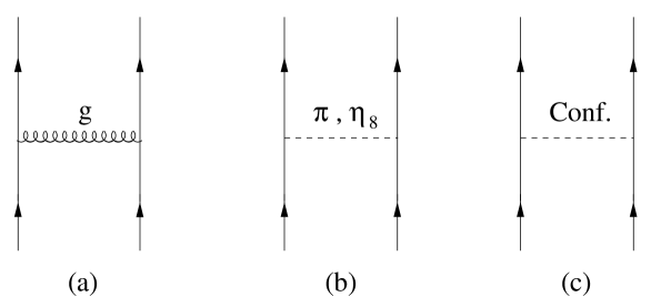
FIG. 1.: Feynman diagrams for two-body exchange potentials. a) One-gluon exchange potential. b) One-pion and one-$\eta_{8}$ exchange potential. c) Confinement potential.

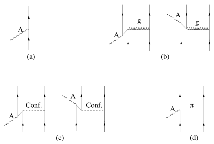
FIG. 2.: Feynman diagrams for the axial operators. a) Impulse. b) One-gluon exchange. c) Confinement interaction. d) Pion exchange.

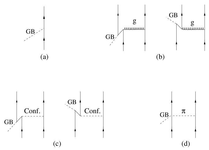
FIG. 3.: Feynman diagrams for the Goldstone boson (GB) absorption operators. a) Impulse. b) One-gluon exchange. c) Confinement exchange. d) Pion exchange.

REFERENCES

- [1] D. Barquilla-Cano, A.J. Buchmann and E. Hernández, Nucl. Phys. A714, 611 (2003).
- [2] J. Ashman et al. (European Muon Collaboration), Phys. Letts. B 206, 364 (1988); Nucl. Phys. B328, 1 (1989).
- [3] K. Abe et al. (E143 Collaboration), Phys. Rev. D 58, 112003 (1998)
- [4] R. D. Carlitz, Int. J. Mod. Phys. E1, 505 (1992).
- [5] H. J. Lipkin, Phys. Lett. B 214, 429 (1988).
- [6] R. Flores-Mendieta, E. Jenkins and A.V. Manohar, Phys. Rev. D 58, 094028 (1996).
- [7] H. E. Jackson, Int. J. Mod. Phys. A17 (2002) 3551. See also the talk by H. E. Jackson in the present proceedings.
- [8] E. Leader and D. B. Stamenov, Phys. Rev. D 67, 037503 (2003)
- [9] A. Manohar and H. Georgi, Nucl. Phys. B234, 189 (1984).
- [10] S. Weinberg, Phys. Rev. Lett. 65, 1181 (1990).
- [11] S. Weinberg, Phys. Rev. Lett. 67, 3473 (1991).
- [12] W. Broniowski, M. Lutz and A. Steiner, Phys. Rev. Lett. 71, 1787 (1993).
- [13] U. Vogl, M. Lutz, S.Klimt and W. Weise, Nucl. Phys. A516, 469 (1990).
- [14] S. Weinberg, “The Quantum Theory of Fields”, Cambridge University Press 1966, Vol II, pags.228-230.
- [15] F. Fernández and E. Oset, Nucl. Phys. A455, 720 (1986).
- [16] W. Weise, Nucl. Phys. A434, 685c (1985).
- [17] A. de Rújula, H. Georgi and S.L. Glashow, Phys. Rev. D 12, 147 (1975).
- [18] N. Isgur and G. Karl, Phys. Rev. D 18, 4187 (1978).
- [19] N. Isgur, G. Karl and R. Koniuk, Phys. Rev. Lett. 41, 1269 (1978); N. Isgur and G. Karl, Phys. Rev. D 19, 2653 (1979).
- [20] U. Meyer, E. Hernández and A. J. Buchmann, Phys. Rev. C64, 035203 (2001).
- [21] H. Yabu, M. Takizawa, W. Weise, Z. Phys. A 345, 193 (1993).
- [22] S. L. Adler, Phys. Rev. 177, 2426 (1969); J. S. Bell and R. Jackiw, Nuo. Cim. A60, 47 (1969); S. L. Adler and W. A. Bardeen, Phys. Rev. 182, 1517 (1969).
- [23] A. Pich, Rept. Prog. Phys. 58, 563 (1995)
- [24] Th. Feldmann, P. Kroll and B. Stech, Phys. Rev. D 58, 114006 (1998).
- [25] A. Bramon, R. Escribano and M. D. Scadron, Eur. Phys. J. C 7, 271 (1999).
- [26] C. McNeile and C. Michael (UKQCD Collaboration), Phys. Lett. B 491, 123 (2000).
- [27] D.E. Groom et al. (Particle Data Group), Eur. Phys. J. C 15, 1 (2000).
- [28] L. Ya. Glozman, W. Plessas, K. Varga and R.F Wagenbrunn, Phys. Rev. D 58, 094030 (1998).
- [29] T. P. Cheng and L.-F. Li, Phys. Rev. Lett. 74, 2872 (1995).
- [30] R. Brockmann and R. Machleidt, Phys. Rev. C 42, 1965 (1990).
- [31] J. C. Peng, Proc. of the LAMPF Workshop on Photon and Neutral Meson Physics at Intermediate Energies-LA-11177-C, Ed. H. W. Baer et al, 1987.
- [32] M. Kirchbach and L. Tiator, Nucl. Phys. A604, 385 (1996).
- [33] S.-L. Zhu, Phys. Rev. C 61, 065205 (2000).
- [34] P. Moskal et al., Phys. Rev. Lett. 80, 3202 (1998).
- [35] Q. Zhao, Phys. Rev. C 63, 035205 (2001).