Abstract

Nuclear pairing correlations are known to play an important role in various single-particle and collective aspects of nuclear structure. After the first idea by A. Bohr, B. Mottelson and D. Pines on similarity of nuclear pairing to electron superconductivity, S.T. Belyaev gave a thorough analysis of the manifestations of pairing in complex nuclei. The current revival of interest in nuclear pairing is connected to the shift of modern nuclear physics towards nuclei far from stability; many loosely bound nuclei are particle-stable only due to the pairing. The theoretical methods borrowed from macroscopic superconductivity turn out to be insufficient for finite systems as nuclei, in particular for the cases of weak pairing and proximity of continuum states. We suggest a simple numerical procedure of exact solution of the nuclear pairing problem and discuss the physical features of this complete solution. We show also how the continuum states can be naturally included in the consideration bridging the gap between the structure and reactions. The path from coherent pairing to chaos and thermalization and perspectives of new theoretical approaches based on the full solution of pairing are discussed.

1 Introduction

Nuclear pairing is one of the main and longstanding pillars of current understanding of nuclear structure. Pairing provides an important contribution to the odd-even mass difference in the phenomenological mass formulae [1]. As an empirical fact the pairing was put in the foundation of the shell model by Mayer and Jensen [2] in order to be able to predict ground state spins and other properties of non-magic nuclei. In the shell-model framework, the classification of paired states is usually performed with the aid of the seniority scheme [3, 4], where the seniority counts a number of unpaired particles; a similar scheme is used in atomic spectroscopy [5]. The Bardeen-Cooper-Schriffer (BCS) microscopic theory of superconductivity [6] elucidated the main features of the ground state, excitation spectrum, transition probabilities and phase transition in a Fermi-system governed by the attractive pairing. Immediately after that A. Bohr, Mottelson and Pines pointed out [7] the similarity between the superconducting pairing correlations and observed pairing effects in nuclei. The thorough application of the BCS approach to the nuclear problem was done by Belyaev in his seminal paper [8]. It was quantitatively demonstrated that the pairing correlations influence nearly all phenomena in low-energy nuclear physics: binding energy, single-particle spectra, transition probabilities, collective vibrational modes, onset of deformation, rotational moment of inertia, level density and thermal properties.

The BCS theory, as well as its advanced form the Hartree-Fock-Bogoliubov (HFB) method [9], is formulated in a way fully appropriate for macroscopic quantum systems; in fact it gives an asymptotically exact solution [10] in the thermodynamic limit. For mesoscopic systems, as nuclei, atomic clusters, quantum dots, Fullerenes, nanotubes or small metallic grains, this approach, although qualitatively reflecting the main physical features, turns out to be insufficient. The total number $N$ of particles is preserved in this method only on average. Since we have to describe the spectroscopy and reactions for a specific nuclide, we need either to add special projection procedures [11, 12, 13, 14] that fix the exact value of $N$ or generalize the formalism by approximately including the matrix elements restoring the particle number conservation [15, 16, 17, 18].

Another drawback of the BCS or HFB approaches is a sharp phase transition as a function of parameters or temperature. As pointed out by Belyaev [8], in a system with a discrete single-particle spectrum, the Cooper phenomenon requires, in contrast to a macroscopic Fermi-gas, a certain minimum strength of pairing attraction. For a weaker pairing, the mean field approaches, as BCS or HFB, give only a trivial normal solution, while in reality the effects of pairing correlations still exist. The pairing correlations in the mean field framework also vanish immediately after the thermal phase transition. These predictions are incorrect for mesoscopic systems. The exact shell model calculations show [19] that the pairing correlations do not disappear at the BCS transition point revealing instead a long tail of “fluctuational superconductivity”.

The main field of interest in nuclear structure is currently shifted to the nuclei far from stability. As we move to loosely bound systems, the influence of the continuum becomes exceedingly important. Along with that, all attractive correlations are to be taken into account properly in order to determine the position of the drip line. The correct treatment of pairing as the main attractive part of the residual interaction is absolutely essential for such problems. Some nuclides, like the notorious ¹¹Li, are bound just due to the pairing correlations between the outermost neutrons, an example of a real Cooper pair [20]. The theory of pairing including both discrete and continuum single-particle levels is still in its infantry [21].

Finally, there is a clear necessity to understand the interplay of pairing with other parts of the residual nuclear interactions going beyond the mean field approximation of the HFB method. Of course, in the lower part of the nuclear chart ($p,sd$ and $pf$ shells) there are well developed modern shell model methods and reliable effective interactions of the nucleons in the truncated single-particle space, see for example [22, 23, 24, 25]. With the possibility of incorporating additional stochastic and statistical elements [26, 27, 28], the shell model calculations are able to describe an impressive amount of spectroscopic data. Unfortunately, the qualitative interpretation of results obtained by the large-scale shell-model diagonalization in terms of simple physical models is getting quite difficult as the matrix dimensions approach the limit of current computational strength. In addition, one needs to mention that the continuum problem is not solved in the standard shell model approach based on the discrete spectrum. Therefore the gap between the shell model for nuclear structure and the reaction theory is widening.

In this situation it is alluring to first separate the pairing part of the nuclear interaction and to solve the corresponding many-body problem exactly. As was shown in [29], the exact solution is numerically simple and eliminates all drawbacks related to the BCS approximation. At the same time, it is still close enough to the standard images of nuclear structure. This exact solution can serve as a zero-order step or a background that allows one to look for the new approaches and approximations to the full problem, effects of other interactions, inclusion of the continuum, relation to the reaction cross sections and so on.

In what follows we start with sketching the traditional approaches and the exact solution of the pairing problem. We compare the exact results with the BCS approximation, both for the ground and excited states, demonstrate the possibility of including the continuum physics and consider chaotic aspects of pairing, a topic practically unexplored in the literature. We complete the paper with the discussion of the perspectives of new approximations based on the exact pairing solution.

2 Approaching the solution of the pairing problem

2.1 Pairing Hamiltonian

We formulate the pairing problem in the restricted single-particle space of fermionic orbitals assuming the Hamiltonian

$$H_{p}=\sum_{1}\epsilon_{1}a^{\dagger}_{1}a_{1}\,-\,\frac{1}{4}\sum_{1,2}G_{12}\,p^{\dagger}_{1}p_{2}.$$ (1)

Here the subscripts 1, … run over the complete set of orthogonal single-particle basis states, and we assume the Kramers double-degeneracy of time-conjugate orbitals $|1)$ and $|\tilde{1})$. The pair creation, $p^{\dagger}_{1}$, and annihilation, $p_{1}$, operators are defined as

$$p^{\dagger}_{1}=a^{\dagger}_{1}a^{\dagger}_{\tilde{1}},\quad p_{1}=a_{\tilde{1}}a_{1},$$ (2)

and the double time-reversal acts as $|\tilde{\tilde{1}})=-|1)$. In the important case of spherical symmetry of the mean field that supports degenerate orbitals $|jm)$ with energies $\epsilon_{j}$, angular momentum $j,$ and projection $j_{z}=m$, the pairing Hamiltonian can be conveniently written as

$$H_{p}=\sum_{j}\,\epsilon_{j}\hat{N}_{j}-\sum_{j\,j^{\prime}}\,G_{jj^{\prime}}L^{\dagger}_{j}L_{j^{\prime}},$$ (3)

where we use the operator notations,

$$\hat{N}_{j}=\sum_{m}\hat{n}_{jm}=\sum_{m}a^{\dagger}_{jm}a_{jm},$$ (4)

for the occupancy operators and ($a_{\tilde{1}}\rightarrow a_{j\tilde{m}}=(-)^{j-m}a_{j-m}$)

$$L_{j}=\frac{1}{2}\sum_{m}(-)^{j-m}a_{j-m}a_{jm},\quad L^{\dagger}_{j}=\frac{1}{2}\sum_{m}(-)^{j-m}a^{\dagger}_{jm}a^{\dagger}_{j-m},$$ (5)

for annihilation and creation operators of pairs in a state with certain quantum numbers of total angular momentum and its projection, $J=M=0$. Essentially the same Hamiltonian (1) can describe the situation in the deformed mean field.

The pairing interaction is defined in terms of real matrix elements of diagonal pair attraction, $G_{11}>0$, and off-diagonal ones, $G_{12}=G_{21}$, for pair transfer between the orbitals 1 and 2. We limit ourselves here by the pairing of identical particles (isospin $T=1$) in states with zero total pair angular momentum; the consideration of the $T=0$ proton-neutron pairing would require a non-zero spin of the pair.

2.2 BCS approach

In the BCS theory, the ground state $|0\rangle_{{\rm BCS}}$ of the paired system with Hamiltonian (1) is determined by minimizing the ground state energy with a trial wave function

$$|0\rangle_{{\rm BCS}}=\Pi_{1>0}(u_{1}-v_{1}p^{\dagger}_{1})|0\rangle=\Pi_{1>0}u_{1}\exp\left(-\frac{v_{1}}{u_{1}}\,p^{\dagger}_{1}\right)|0\rangle\,,$$ (6)

where the variational parameters for each pair of time-conjugate orbitals, $u_{1}$ and $v_{1}$, can be taken as real numbers subject to the normalization $u_{1}^{2}+v_{1}^{2}=1$. In our discussion we denote $|N;s\dots\rangle$ as the lowest in energy $N$-particle state with quantum numbers $s,\dots.$ We use the notation $|s\rangle_{{\rm BCS}}$ for the BCS state with $s$ quasiparticles that has an uncertain particle number; for this reason $N$ is not shown, however it is assumed that the state corresponds to an average particle number $\overline{N}.$ The restriction $1>0$ means that the time-conjugate orbitals are not counted twice. The exponential form of the variational wave function shows that this state is generated as a coherent state of fermionic pairs; this feature can be put in a foundation of methods going beyond the BCS [30, 31].

The variational solution is given via the occupation amplitudes

$$v_{1}^{2}=n_{1}=\frac{1}{2}\left(1-\frac{\epsilon_{1}}{e_{1}}\right),\quad u_{1}^{2}=1-n_{1}=\frac{1}{2}\left(1+\frac{\epsilon_{1}}{e_{1}}\right),$$ (7)

where $e_{1}=\sqrt{\epsilon_{1}^{2}+\Delta_{1}^{2}}$ is quasiparticle energy and $\Delta_{1}$ is the BCS energy gap. The gap equation arising from the minimization of energy is

$$\Delta_{1}=\frac{1}{2}\,_{{\rm BCS}}\langle 0|\sum_{2}G_{1\,2}\,p^{\dagger}_{2}|0\rangle_{{\rm BCS}}=\sum_{2}\frac{G_{1\,2}}{2e_{2}}\,\Delta_{2}.$$ (8)

The ground state as well as low-lying excited states of paired systems can be classified introducing quasiparticle creation operators

$$\alpha^{\dagger}_{1}=u_{1}a^{\dagger}_{1}-v_{1}a_{\tilde{1}}\,.$$ (9)

This transformation is canonical due to the correct normalization of $u$ and $v$. The BCS vacuum $|0\rangle_{{\rm BCS}}$ in (6) can be defined as $\alpha|0\rangle_{{\rm BCS}}=0\,.$ The Bogoliubov transformation (9) mixes particle and hole states.

One of the problems in the BCS application to small systems is particle number non-conservation which follows from the form of the wave function (6). A common practice to fix the number of particles is to introduce a chemical potential $\mu$ by the shift of single-particle energies $\epsilon\rightarrow\epsilon-\mu.$ The right total particle number is restored in average through the condition

$$\sum_{1}n_{1}(\mu)=\overline{N}.$$ (10)

The uncertainty of the total particle number is given by

$$(\Delta N^{2})=\overline{N^{2}}-{\overline{N}}^{2}=\sum_{1}n_{1}(1-n_{1})\,.$$ (11)

Practically this fluctuation is of the order $\sqrt{(\Delta N^{2})}\approx 2\,.$ Given that relative fluctuations go down with increasing $N\,,$ the BCS solution is asymptotically exact in the thermodynamic limit of macroscopic systems [10]. The contribution to the energy from the fluctuation is quadratic in the number of particles [32] and thus gives an extra correction of the monopole type. Special methods, such as Lipkin-Nogami [11, 12] techniques, were invented in order to suppress the particle number fluctuations.

The particle number violation in the BCS is an example of spontaneous symmetry breaking with respect to phase rotations generated by the number operator, $U(\phi)=\exp(-i\phi\hat{N}/2)\,.$ While the pairing Hamiltonian is invariant under this rotation, $[H_{p},\,U(\phi)]=0\,,$ the trial ground state $|0\rangle_{{\rm BCS}}$ has a preferred orientation, with the usual consequences of the appearance of Anderson-Goldstone-Nambu modes whose properties are influenced by the mesoscopic nature of the nuclear systems [33]. A number of projection techniques have been developed within the framework of the symmetry violation treatment, see [34] and references therein.

2.3 Recursive method with particle number conservation

Instead of introducing the pair condensate of the pairs with an uncertain particle number, another possibility was explored [35, 36, 17], where the matrix elements of relevant operators explicitly keep memory of the exact particle number. The gap is defined now as a matrix element of the pair annihilation operator between the ground states $|N;0\rangle$ of the neighboring even systems,

$$\Delta_{1\,}(N)=\frac{1}{2}\,\langle N-2;0|\sum_{2}\,G_{1\,2}\,p_{2}|N;0\rangle\,.$$ (12)

Similarly, the particle number dependence enters the single-particle transition amplitudes between adjacent even and odd systems,

$$v_{1\,}(N)=\langle N-1;\tilde{1\,}|a_{1\,}|N;0\rangle,\,\quad u_{1\,}(N)=\langle N+1;1\,|a^{\dagger}_{1\,}|N;0\rangle\,.$$ (13)

Here one needs to consider a sequence of ground states $|N;0\rangle$ with energies $E(N)\,$. It is assumed that the spectra of adjacent odd nuclei start with energies $E(N\pm 1;\,1\,)$ of the states $|N\pm 1;1\,\rangle$ containing one unpaired nucleon with quantum numbers 1.

The exact operator equations of motion for the single-particle operators $a_{1}\,$ and $a^{\dagger}_{1}\,$,

$$[a_{1}\,,\,H]=\epsilon_{1}\,a_{1}\,\,+\,\frac{1}{2}\sum_{2}\,G_{1\,2}\,a^{\dagger}_{\tilde{1\,}}\,p_{2}\,,$$ (14)

$$[a^{\dagger}_{1\,},\,H]=-\epsilon_{1}\,a_{1}^{\dagger}\,-\,\frac{1}{2}\sum_{2}\,G_{1\,2}\,p^{\dagger}_{2}\,a_{\tilde{1\,}},$$ (15)

can be used to construct recursive in $N$ equations for the gap (12) and single-particle transition amplitudes (13). The approximation of no condensate disturbance by an extra particle [35, 36],

$$\langle N-1;1\,|\sum_{2}\,G_{1\,2}\,a^{\dagger}_{\tilde{1\,}}\,p_{2}|N;0\rangle$$

$$\approx\langle N-1;1\,|a^{\dagger}_{\tilde{1\,}}|N-2;0\rangle\langle N-2;0|\sum_{2}\,G_{1\,2}\,\,p_{2}|N;0\rangle=2\Delta_{1\,}(N)\,u_{\tilde{1\,}}(N-2),$$ (16)

leads to the recursion relation connecting adjacent even nuclei,

$$\left|v_{1\,}(N-2)\right|^{2}=1-\frac{\left|\Delta_{1\,}(N)\right|^{2}}{[e_{1\,}(N)-{\epsilon^{\prime}}_{1\,}(N)]^{2}}\left|v_{1\,}(N)\right|^{2}\,,$$ (17)

where the $N$-dependent chemical potential is introduced,

$$\mu(N)=\frac{1}{2}\left(E(N)-E(N-2)\right),$$ (18)

and quasiparticle excitation energy is defined as

$$e^{2}_{1\,}={{\epsilon^{\prime}_{1}(N)}^{2}+|\Delta_{1\,}(N)|^{2}}\,,$$ (19)

with shifted single-particle energies

$$\epsilon_{1}^{\prime}(N)=\epsilon_{1\,}-\frac{G_{1\,1\,}}{2}-\mu(N)\,.$$ (20)

The analogs of the number conservation equation and the gap self-consistency condition now read

$$\Omega-N+2=\sum_{1\,}\frac{\left|\Delta_{1\,}(N)\right|^{2}}{[e_{1\,}(N)-{\epsilon^{\prime}}_{1\,}(N)]^{2}}\left|v_{1\,}(N)\right|^{2},$$ (21)

where $\Omega$ is the total capacity of fermionic space, and

$$\Delta_{1\,}(N)=\frac{1}{2}\,\sum_{2}\,G_{1\,2}\frac{\Delta_{2}(N)\,\left|v_{2}(N)\right|^{2}}{e_{2}(N)-{\epsilon^{\prime}}_{2}(N)}\,.$$ (22)

The pairing problem formulated in this manner allows a recursive solution in both directions, starting from the empty shell or from the completely filled shell. This solution reduces to the BCS under assumption that the gap does not change in the transition from $N$ to $N-2,$ the same approximation of particle number uncertainty that lead to the BCS particle number fluctuation (11). Based on this feature, the BCS energy can be efficiently corrected by the substitution $\overline{N}\rightarrow\overline{N}-1$ [37]. Corrections to such iterative methods via inclusion of pair-vibration excitations in the intermediate states of Eq. (16) with further diagonalization are also possible [17], as well as the treatment of the excitations with RPA techniques [38, 39].

The particle conserving treatment does not resolve another problem of the BCS solution, namely the sudden disappearance of pairing correlations when coupling becomes too weak. The gap equations, (8) and (22), have only trivial $\Delta=0$ solutions if the pairing strength $G$ is too small compared to the single-particle energy spacings. The point of this phase transition is roughly at the critical coupling strength $G_{c}$,

$$G_{c}\,\nu_{\rm F}=1,$$ (23)

where both the pairing strength and the density of single-particle states $\nu_{\rm F}$ are taken at Fermi energy. Many nuclear systems in the shell model picture are close to or even below the point of the BCS instability, although the pairing correlations do still exist [29]. As will be discussed later, near the phase transition, in the so-called pair-vibrational regime, the fluctuations drive pair scattering to an almost chaotic level leading to a sharp increase of the mixing between the states of the same seniority. This randomness makes the approximation (16) or any truncation of states mixed by the pair vibrations inappropriate. Various projection techniques also seriously suffer in the region of weak pairing. More advanced approaches, such as HFB+RPA, break down in the vicinity of the phase transition, though the pairing solution can still be continued into the region beyond the critical point using the RPA based on the Hartree-Fock solution for a normal state. This treatment drastically improves the prediction for the ground state energy [40]. The methods of equations of motion [32, 41] and variational techniques can be used to better account for the RPA ground state correlations [42]. Being applied to superfluid Fermi systems these methods demonstrated a considerable improvement [42, 43].

3 Exact solution of the pairing problem

Historically, a few suggestions were put forward for the exact solution of the pairing problem. The Richardson method, described in the series of papers [44, 45], provides a formally exact way for solving the pairing Hamiltonian. This method reduces the large-scale diagonalization of a many-body Hamiltonian matrix in a truncated Hilbert space to a set of coupled equations ($\Omega_{j}=2j+1$)

$$\sum_{j}\frac{\Omega_{j}}{2\epsilon_{j}-z_{\lambda}}-\sum_{\lambda^{\prime}\neq\lambda}\,\frac{4}{z_{\lambda^{\prime}}-z_{\lambda}}=\frac{2}{G}\,$$ (24)

for unknown parameters $z_{\lambda}\,,$ their number being equal to that of valence particle pairs. The ground state energy is then equal to $E(N)=\sum_{\lambda}^{N/2}\,z_{\lambda}\,.$

Recently this solution was revived and reinterpreted [46] with the aid of the electrostatic analogy, similar to that used by Dyson in his theory [47] of random level ensembles. Unfortunately, the Richardson solution is only valid for the constant pairing force, $G_{jj^{\prime}}=G=\,$const. It also requires serious numerical efforts rapidly growing with the number of particles. Recently, exact solutions have been also approached with sophisticated mathematical tools as infinite-dimensional algebras [48]. Such formally exact solutions have a certain merit from a mathematical point of view and might be useful for developing simple models [49, 50]. However, they are not very promising for practical problems in nuclear physics.

The natural way of solving the pairing problem is related to the direct Fock-space diagonalization. For deformed nuclei with the doubly degenerate single-particle orbitals this approach supplemented by the appropriate use of symmetries and truncations was already shown to be quite effective [51, 52]. The diagonalization of the general pairing Hamiltonian (3) is much simpler than that of the full shell-model Hamiltonian due to the possibility of classifying many-body states within the seniority scheme [3, 4, 53], especially in the case of spherical symmetry (3). Long ago it was shown [53, 54] that this approach is useful not only in the exactly solvable degenerate model but in a realistic shell model context as well. With a perspective to complement the pairing problem with the subsequent account for other parts of the residual interaction, we consider this path promising and quite practical.

It is well known that the pair annihilation, $L_{j}$, pair creation $L^{\dagger}_{j}$, and occupation number operator (shifted to the middle of the $j$-subshell),

$$L_{j}^{\circ}=\frac{1}{2}\hat{N}_{j}-\frac{1}{4}\Omega_{j},\quad\Omega_{j}=2j+1,$$ (25)

form an SU(2) algebra of “quasispin” for each $j$-subshell,

$$[L_{j},L^{\circ}_{j^{\prime}}]=\delta_{jj^{\prime}}L_{j},\quad[L^{\dagger}_{j},L^{\circ}_{j^{\prime}}]=-\delta_{jj^{\prime}}L^{\dagger}_{j},\quad[L_{j},L^{\dagger}_{j^{\prime}}]=-2\delta_{jj^{\prime}}L^{\circ}_{j}.$$ (26)

Therefore the pairing Hamiltonian (3) preserves all partial quasispins $\Lambda_{j}$,

$${\bf L}_{j}^{2}=(L^{\circ}_{j})^{2}+\frac{1}{2}(L_{j}^{\dagger}L_{j}+L_{j}L^{\dagger}_{j})=\Lambda_{j}(\Lambda_{j}+1).$$ (27)

The partial seniority quantum numbers,

$$s_{j}=\frac{\Omega}{2}-2\Lambda_{j},$$ (28)

are also conserved. They express the number of unpaired, and therefore not participating in the pairing interaction (3), particles. The fully paired $j$-level corresponds to the maximum partial quasispin $\Lambda_{j}=\Omega/4$ and lowest partial seniority $s_{j}=0$.

The pair transfer $L^{\dagger}_{j^{\prime}}L_{j}$ between the levels $j\rightarrow j^{\prime}$ changes the occupancies, i.e. projections $L^{\circ}_{j}$ and $L^{\circ}_{j^{\prime}}$, keeping intact the lengths of quasispins $\Lambda_{j}$ and $\Lambda_{j^{\prime}}$, and, whence, seniorities $s_{j}$ and $s_{j^{\prime}}$. The space is decomposed into sectors with given partial seniorities $s_{j}$, and the basis states within each sector can be labelled by the set of occupancies $N_{j}$ under a constraint $\sum_{j}N_{j}=N$, the total valence particle number. The passive (unpaired) particles occupy fixed orbitals and create nonzero seniorities. They influence the dynamics indirectly, through the Pauli blocking. The states with zero total seniority $s=\sum_{j}s_{j}$ have the total spin $J=0$, while for $s\neq 0$ the further decomposition with respect to the rotation group is possible, and some many-body states with different angular momentum coupling but the same seniorities remain degenerate.

Using the states with given values of $s_{j}$ and various possible occupancies $N_{j}$ as a basis, it is easy to construct the Hamiltonian matrix that is essentially the matrix with respect to the sets of $N_{j}$. The diagonal matrix elements are

$$\langle\{s_{j}\},\{N_{j}\}|H_{p}|\{s_{j}\},\{N_{j}\}\rangle=\sum_{j}\left[\epsilon_{j}N_{j}-\frac{G_{jj}}{4}(N_{j}-s_{j})(\Omega_{j}-s_{j}-N_{j}+2)\right].$$ (29)

Each term in the square brackets gives a full solution for the pairing problem on a degenerate $j$-level. Clearly, as long as seniority is small, $s_{j}\ll\Omega_{j}$, each unpaired particle increases energy by $\Delta_{j}=G_{jj}\Omega_{j}/4$, and this quantity plays the role analogous to that of the energy gap in the BCS theory. The off-diagonal matrix elements for the pair transfer $j^{\prime}\rightarrow j$ are

$$H_{j^{\prime}\rightarrow j}=-\frac{G_{jj^{\prime}}}{4}\left[(N_{j^{\prime}}-s_{j^{\prime}})(\Omega_{j^{\prime}}-s_{j^{\prime}}-N_{j^{\prime}}+2)(\Omega_{j}-s_{j}-N_{j})(N_{j}-s_{j}+2)\right]^{1/2}.$$ (30)

The highest matrix dimension is encountered for the lowest possible total seniority, $s=0$ for an even number of particles, and $s=1$ for an odd number of particles. But, even for heavy nuclei, this dimension does not exceed few thousand (in modern shell model computations one has to deal with dimensions $10^{8}$ and higher in the $m$-scheme). In addition, the Hamiltonian matrix is very sparse. As a result of the numerical diagonalization we obtain the spectrum of states for a given set of seniorities. For example, for an even system, the condition $s=0$ selects all zero partial seniorities, $s_{j}=0$. All those states correspond to pair condensates that differ by the distribution of the average partial occupancies $\{N_{j}\}$ among the subshells. In a standard language of the BCS theory supplemented by the random phase approximation (RPA), the excited states for $s=0$ are various pair vibrations. However, here we do not make any assumptions of boson character or harmonic spectrum of excitations. The next section illustrates the typical results of the diagonalization.

4 Example: A chain of even isotopes

The longest known chain of tin isotopes is a subject of extensive experimental and theoretical studies. Even considering the proton subsystem, $Z=50$, as an inert core, we have to deal with the neutron model space that is too large for a direct diagonalization. Modern computational techniques that use the Lanczos iteration method allow for exact determination of few low-lying states in systems with up to 12 valence particles [55]. These results are essential for testing the approximate techniques. It is known that pairing correlations play a major role in forming the ground state wave functions of tin isotopes.

$$\begin{array}[]{c|ccccc}&g_{7/2}&d_{5/2}&d_{3/2}&s_{1/2}&h_{11/2}\cr\epsilon_{j}&-6.121&-5.508&-3.749&-3.891&-3.778\cr\hline\cr g_{7/2}&0.9850&0.5711&0.5184&0.2920&1.1454\cr d_{5/2}&&0.7063&0.9056&0.3456&0.9546\cr d_{3/2}&&&0.4063&0.3515&0.6102\cr s_{1/2}&&&&0.7244&0.4265\cr h_{11/2}&&&&&1.0599\cr\end{array}$$

Table 1: Single-particle energies and pairing matrix elements $V_{0}(jj;j^{\prime}j^{\prime})$ (in MeV) for the shell model space from ¹⁰⁰Sn to ¹³²Sn; matrix elements are determined from $G$-matrix calculations.

Unlike in many other nuclear systems, pairing in tin isotopes is quite strong and stable being sufficiently above the point of the BCS phase transition. There is only a relatively minor weakening in the mass region near ¹¹⁴Sn due to a gap between $d_{5/2}$ and $g_{7/2}$ and the rest of single-particle orbitals. We specifically would like to explore this region in order to discuss physics of the BCS phase transition.

For tin isotopes ranging in mass number from $A=100$ to $A=132$, we assume a configuration space between the two neutron magic numbers, 50 and 82. The valence neutron space contains here five single-particle orbitals, $h_{11/2},\,d_{3/2},\,s_{1/2},\,g_{7/2},$ and $d_{5/2}\,.$ We adopt parameters shown in Table 1, the single-particle energies taken from experimental data and the interaction matrix elements from the $G$-matrix calculation [55]. The interaction parameters $V_{0}$ in Table 1 are related to the pairing strengths $G_{jj^{\prime}}$ as

$$G_{jj^{\prime}}=\frac{1}{2}V_{0}(jj;j^{\prime}j^{\prime})\sqrt{(2j+1)(2j^{\prime}+1)}.$$ (31)

The shell model calculations with these parameters reproduce the spectroscopy of tin isotopes in the region $A=120$ to $A=130$ with a good accuracy. In parallel we discuss similar effects in calcium isotopes where we used a well established FPD6 interaction [24]. The $fp$ neutron valence space covers calcium isotopes from ⁴⁰Ca to ⁶⁰Ca. The weakening of pairing in Ca occurs near ⁴⁸Ca, i.e. for the $f_{7/2}$ subshell closure. Results of the calculation for the ¹¹⁴Sn region are shown in Table 2 and for the region ⁴⁸Ca in Table 3.

$$\begin{array}[]{c|c|ccccc}\hline\cr&&g_{7/2}&d_{5/2}&d_{3/2}&s_{1/2}&h_{11/2}\cr\hline\cr\hline\cr&EP:&&&&&\cr\hline\cr({\rm a})&N_{j}(N)&6.96&4.46&0.627&0.356&1.6\cr({\rm b})&n_{j}(N)&0.870&0.744&0.157&0.178&0.133\cr({\rm c})&u^{2}_{j}(N)&0.128&0.252&0.838&0.817&0.863\cr({\rm d})&v^{2}_{j}(N)&0.865&0.736&0.155&0.177&0.131\cr({\rm e})&S_{j}(N+1)&2.8&3.13&3.14&3.39&3.29\cr({\rm f})&S_{j}(N)&6.86&6.55&7.25&6.98&7.12\cr({\rm g})&|\langle N+2;0|P^{\dagger}_{j}|N;0\rangle|&0.68&0.779&0.617&0.514&1.03\cr({\rm h})&|\langle N;0|P_{j}|N-2;0\rangle|&0.81&0.93&0.524&0.396&0.845\cr\hline\cr\hline\cr&BCS:&&&&&\cr\hline\cr({\rm i})&N_{j}(N)&6.71&4.14&0.726&0.507&1.91\cr({\rm j})&n_{j}(N)&0.839&0.69&0.181&0.254&0.159\cr({\rm k})&\Delta_{j}&1.31&1.43&1.43&1.38&1.25\cr({\rm l})&e_{j}&1.78&1.55&1.86&1.59&1.71\cr({\rm m})&S_{j}(N+1)&2.89&3.21&3.11&3.21&3.26\cr({\rm n})&S_{j}(N)&6.89&6.64&7.2&7.03&7.06\cr({\rm o})&{}_{{\rm BCS}}\langle 0|P_{j}|0\rangle_{{\rm BCS}}&0.734&0.801&0.545&0.435&0.896\cr\hline\cr\end{array}$$

EP: $E(^{114}{\rm Sn})=-86.308,\;E(^{116}{\rm Sn})=-95.942,\;E(^{112}{\rm Sn})=-75.831.$
BCS: $E(^{114}{\rm Sn})=-85.938,\;\mu=-5.035$.

Table 2: The results of the exact pairing solution (EP) compared to the BCS solution for the ¹¹⁴Sn nucleus; the interaction matrix elements are determined by the $G$-matrix calculations, see text; the separation energies $S_{j}$, quasiparticle energies $e_{j}$ and the pairing gaps $\Delta_{j}$ are given in MeV.

An important consequence of the proximity to the BCS phase transition is a reduction of pairing correlation energy predicted by the BCS but not confirmed by the exact solution. In the tin example the BCS underpredicts binding energy by about 0.4 MeV, while for calcium this number reaches 0.6 MeV. A similar difference appears in one-nucleon separation energy $S_{j}(N)=E(N-1)-E(N)$ (index $j$ here denotes the orbital of the unpaired nucleon in an odd-$N$ system), as can be seen from the comparison of rows (e) and (f) with the corresponding BCS prediction, lines (m) and (n), Tables 2 and 3. As stressed in Ref. [29], this discrepancy can be crucial for the nuclei near drip lines. Unfortunately, the BCS hardly can be improved with respect to the treatment of weak pairing. Even for the complicated particle number projection techniques accompanied by the the variational procedures on a broader set of mean field states, it remains unclear to what extent it is possible to describe the pairing phase transition, and whether the high-lying pair vibrations are included, the step needed to account for missing correlation energy.

$$\begin{array}[]{c|c|cccc}\hline\cr&j&7/2&3/2&5/2&1/2\cr&\epsilon_{j}&-8.39&-6.5&-1.9&-4.48\cr\hline\cr\hline\cr&EP:&&&&\cr\hline\cr({\rm a})&N_{j}(N)&6.87&0.85&0.173&0.111\cr({\rm b})&n_{j}(N)&0.858&0.212&0.0288&0.0557\cr({\rm c})&u^{2}_{j}(N)&0.133&0.779&0.97&0.939\cr({\rm d})&v^{2}_{j}(N)&0.848&0.212&0.0281&0.0555\cr({\rm e})&S_{j}(N+1)&4.48&5.78&1.55&4.09\cr({\rm f})&S_{j}(N)&9.64&9.75&14.1&11.5\cr({\rm g})&\langle N+2;0|P^{\dagger}_{j}|N;0\rangle&0.706&0.928&0.289&0.309\cr({\rm h})&\langle N;0|P_{j}|N-2;0\rangle&1.07&0.612&0.288&0.232\cr\hline\cr\hline\cr&BCS:&&&&\cr\hline\cr({\rm i})&N_{j}(N)&6.5&1.22&0.155&0.124\cr({\rm j})&n_{j}(N)&0.813&0.304&0.0258&0.062\cr({\rm k})&\Delta_{j}&1.66&1.44&1.73&1.53\cr({\rm l})&e_{j}&2.13&1.56&5.45&3.18\cr({\rm m})&S_{j}(N+1)&4.5&5.66&1.64&4.1\cr({\rm n})&S_{j}(N)&9.64&9.51&13.8&11.3\cr({\rm o})&{}_{{\rm BCS}}\langle 0|P_{j}|0\rangle_{{\rm BCS}}&0.78&0.651&0.275&0.241\cr\hline\cr\end{array}$$

EP: $E(^{48}{\rm Ca})=-71.215,\;E(^{50}{\rm Ca})=-85.149,\;E(^{46}{\rm Ca})=-55.501$.
BCS: $E(^{48}{\rm Ca})=-70.591,\;\mu=-7.335.$

Table 3: Properties of the weakly-paired ⁴⁸Ca nucleus; the FPD6 interaction was used in these calculations; all energies are given in MeV.

Another related feature is the difference in predicted occupation numbers that can be inferred from comparing rows (a) and (b) with (i) and (j) in Tables 2 and 3. A proper account for this difference can partially help to correct the binding energy. In the presence of additional interactions, the monopole contribution to the energy can be particularly sensitive to the precise occupation numbers. Furthermore, in the use of mean-field methods for paired systems, a good reconstruction of the density matrix generated by the pairing is of critical importance.

The exact pairing treatment (EP) becomes increasingly important in considering the reaction amplitudes with paired nuclei. The one-nucleon transition amplitudes defined in the exact solution via Eq. (13) can be compared with the corresponding BCS quantities. Since, similarly to the recursive approach, these amplitudes connect different nuclei, the standard BCS relations $v^{2}_{j}=n_{j}$, $u_{j}^{2}=1-n_{j}$ and $u_{j}^{2}+v^{2}_{j}=1$ are no longer true. Deviations from these equalities are clearly enhanced in the phase transition region where adding an extra particle can make a sharp difference. The BCS theory with an uncertain particle number does not account for such effects. The pair emission amplitudes exhibit even larger differences. Rows (g) and (h) of the Tables 2 and 3 show these amplitudes for adjacent even systems. The numbers are noticeably different (in the BCS approach they are substituted with a single set shown in row (o)). These discrepancies are particularly crucial for weakly bound nuclei since not only the binding energy is affected by the improved treatment of pairing but also there are significant corrections to the reaction amplitudes.

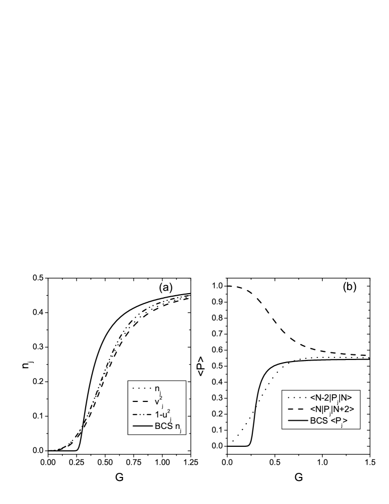
Figure 1: Comparison of BCS and EP solutions for the ladder system as a function of pairing strength $G$. In panel (a) occupation numbers for the sixth level (first level above the Fermi surface) and spectroscopic factors for capture and decay are compared to exact calculation. For the same level, the pair emission and pair absorption amplitudes are compared, panel (b), to the BCS prediction.

Further insight into the situation can be gained by varying the coupling strength. For this purpose we consider a “ladder” model that contains ten double-degenerate single-particle orbitals equally spaced with the interval of a unit of energy. The valence space is assumed to be half-occupied with $N=10$ particles. The most interesting region is near the Fermi surface, $\epsilon_{\rm F}=5.$ For Fig. 1 we consider the first single-particle level above the Fermi energy. As in the previous example, the BCS result significantly deviates from the exact solution near the phase transition, around $G=0.5$, as seen from panel (a). In the same region one can observe a slight difference between $v_{j}^{2}$, $1-u_{j}^{2}$ and $n_{j}$ in the exact solution. For the pair emission process, the differences between the BCS and exact solution become more pronounced. Here the particle number uncertainty is crucial since the level under consideration is above Fermi energy for $N=10$, but below it for $N=12$.

Figure 2: Matrix elements of the operator $N_{j}$ for the $d_{5/2}$ level in ¹¹⁴Sn between the ground state and all pair vibrational states $\phi$ (zero seniority) plotted as a function of excitation energy of the state $\phi$.

Contrasting the exact solution with the mean field picture, we can notice that the occupation number operators $\hat{N}_{j}$ in general may have nonzero off-diagonal matrix elements between states of the same seniority. In Figs. 2, ¹¹⁴Sn, and 3, the ladder model, the matrix elements between the ground state and all $s=0$ states are shown as a function of excitation energy. In all cases the off-diagonal matrix elements rapidly fall off. In the case of weak pairing (Fig. 3, circles), one can still see the structure of excited states based on the equidistant single-particle spectrum. For stronger pairing (compared to the single-particle level spacing), Fig. 3, triangles, as well as in the realistic case for spherical symmetry, Fig. 2, the decrease of matrix elements is more uniform and can be approximated in average by an exponential function of excitation energy. This indicates chaotization of motion even in the sector with seniority $s=0$, [56]. Only very few states with relatively large matrix elements may carry pair-vibrational features. As follows from the extended shell model analysis [57], the exponential tails of the strength functions are typical for many-body quantum chaos [58]. The property of exponential convergence was demonstrated in Ref. [28] and the extrapolation based on this property was later used [59, 60, 61] as a practical tool for getting reliable quantitative results in shell-model calculations of intractable large dimensions.

Figure 3: Matrix elements of $N_{6}$ (the sixth single-particle state in the ladder model) between the ground state and excited $s=0$ states as a function of excitation energy.

5 Continuum effects

As the main interest of low-energy nuclear physics is moving to nuclei far from the valley of stability, the continuum effects become exceedingly important for a unified description of the structure of barely stable nuclei and corresponding nuclear reactions. The pairing part of the residual interaction in some cases is the main source of the nuclear binding; spectroscopic factors and reaction amplitudes are also critically dependent on pairing.

As a demonstration of a realistic shell-model calculation combining the discrete spectrum and the continuum, we consider oxygen isotopes in the mass region $A=16$ to 28. In this study we use a universal $sd$-shell model description with the semi-empirical effective interaction (USD) [25]. The model space includes three single-particle orbitals $1s_{1/2}$, $0d_{5/2}$ and $0d_{3/2}$ with corresponding single-particle energies $-3.16,\;-3.95$ and 1.65 MeV. The residual interaction is defined in the most general form with the aid of a set of 63 reduced two-body matrix elements in pair channels with angular momentum $L$ and isospin $T$, $\langle(j_{3}\tau_{3},j_{4}\tau_{4})LT|V|(j_{1}\tau_{1},j_{2}\tau_{2})LT\rangle$, that scale with nuclear mass as $(A/18)^{-0.3}$.

In the discrete spectrum the full shell model treatment is possible for such light systems. Aiming at the study of the continuum effects, that increase significantly the computational load, here we truncate the shell-model space to include only seniority $s=0$ and $s=1$ states. This method, “exact pairing + monopole”, is known [29] to work well for shell model systems involving only one type of nucleons (in the case of the oxygen isotope chain only neutrons and the interaction matrix elements with isospin $T=1$ are involved). The two important ingredients of residual nuclear forces are treated by this method exactly: the monopole interaction that governs the binding energy behavior throughout the mass region, and pairing that is responsible for the emergence of the pair condensate, renormalization of single-particle properties and collective pair vibrations.

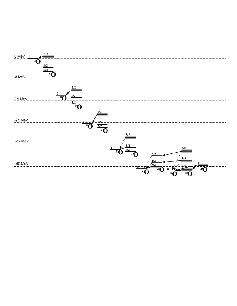
Figure 4: Schematic picture of lowest seniority states and possible decays in oxygen isotopes. Dotted arrows indicate the decays blocked by seniority conservation.

In the resulting simplified shell-model description, the set of the original 30 two-body matrix elements in the $T=1$ channel is reduced to 12 most important linear combinations. Six of these are the two-body matrix elements for pair scattering in the $L=0$ channel describing pairing, and the other six correspond to the monopole force in the particle-hole channel,

$$\overline{V}_{j,j^{\prime}}\equiv\sum_{L\neq 0}(2L+1)\langle(j,j^{\prime})L1|V|(j,j^{\prime})L1\rangle,$$ (32)

where $j$ and $j^{\prime}$ refer to one of the three single-particle levels.

We assume here that the $0d_{3/2}$ orbital belongs to the single-particle continuum and therefore its energy has an imaginary part. In this model we account for two possible decay channels $|c\rangle$ for each initial state $|\Phi\rangle$, a one-body channel, $c=1$, and a two-body channel, $c=2$. The one-body decay changes the seniority of the $0d_{3/2}$ orbital from 1 to 0 in the decay of an odd-$A$ nucleus and from 0 to 1 for an even-$A$ nucleus. The two-body decay with the zero angular momentum of the pair removes two paired particles and does not change the seniority. The two channels lead to the lowest energy state of allowed seniority in the daughter nucleus; transitions to excited pair-vibrational states are ignored. This results in

$$e_{3/2}(\Phi)=\epsilon_{3/2}-\frac{i}{2}{\alpha_{3/2}}\,(E_{\Phi}-E^{(1)})^{5/2}-i\,\alpha_{3/2}(E_{\Phi}-E^{(2)})^{5/2}\,,$$ (33)

where we assumed that one- and two-body decay parameters $\gamma^{(c)}_{j}$ are related as $\gamma^{(1)}_{3/2}=\gamma^{(2)}_{3/2}/2\equiv\gamma_{3/2}$, and the particles are emitted in the $d$-wave with $\ell=2\,$. The energy dependence of the widths near decay thresholds $E^{(c)}$ is very important; $\alpha_{3/2}$ is the reduced width parameter that differs from $\gamma_{3/2}$ by the absence of the energy factor. Three states with the valence particle at one of the single-particle orbitals can be identified as the $5/2^{+}$ ground state and $1/2^{+}$ and $3/2^{+}$ excited states in the spectrum of ¹⁷O. Their energies relative to ¹⁶O correspond to the single-particle energies in the USD model. Experimental evidence indicates that the $3/2^{+}$ state decays via neutron emission with the width $\Gamma(^{17}$O$)=96$ keV. This information allows us to fix our parameter $\alpha_{3/2}=\Gamma(^{17}$O$)/(\epsilon_{3/2})^{5/2}=0.028$ (MeV)${}^{-3/2}\,.$ Other two states are particle-bound, $\gamma_{1/2}=\gamma_{5/2}=0\,.$

With complex single-particle energies, the non-Hermitian effective Hamiltonian for the many-body system is constructed in a regular way [62, 63]. The Hamiltonian includes the Hermitian pairing and monopole terms as well as the energy-dependent non-Hermitian effective interaction through the open decay channels, the structure of which is dictated by unitarity [63]. Energy dependence is determined by the proximity of thresholds, Eq. (33). We move along the chain of isotopes starting from ¹⁶O. In this way, for each $A$ the properties of the possible daughter systems $A-1$ and $A-2$ are known. The chain of isotopes under consideration is shown in Fig. 4, which includes $s=0$ and $s=1$ states and indicates possible decays. The decays indicated by the dotted arrows are blocked in our model due to the exact seniority conservation. Non-pairing interactions in the full shell model mix seniorities making these decays possible. Since the effective Hamiltonian depends on energy and all threshold energies have to be determined self-consistently, we solve this extremely non-linear problem iteratively. We start from the shell-model energies $E_{{\rm s.m.}}$ corresponding to a non-decaying system. Then the diagonalization of the Hamiltonian at this energy allows us to determine the next approximation to the complex energies ${\cal E}=E-(i/2)\Gamma$ that give the position and the width of a resonance. This cycle is repeated until convergence that is usually achieved in less than ten iterations.

The results of the calculations and comparison with experimental data for oxygen isotopes are shown in Table 4. Despite numerous oversimplifications related to seniority truncation, limitations on the configuration mixing and restrictions on possible decay channels and final states, the overall agreement observed in Table 4 is quite good. If experimental data are not available, the results can be considered as predictions. The main merit of this calculation is in demonstrating the power and practicality of the EP method extended to continuum problems. The same calculation predicts also [64] the cross sections of the processes related to the included channels providing the unified description of the structure and reactions with loosely bound nuclei.

$$\begin{array}[]{|r|r|r|r||r|r|}\hline\cr A&J&E\,{\rm(MeV)}&\Gamma\,{\rm(keV)}&E_{\rm exp.}\,{\rm(MeV)}&\Gamma_{\rm exp.}\,{\rm(keV)}\\ \hline\cr 16&0&{\bf 0.00}&0&{\bf 0.00}&0\\ 17&5/2&{\bf-3.94}&0&{\bf-4.14}&0\\ 17&1/2&0.78&0&0.87&0\\ 17&3/2&5.59&96&5.08&96\\ 18&0&{\bf-12.17}&0&{\bf-12.19}&0\\ 19&5/2&{\bf-15.75}&0&{\bf-16.14}&0\\ 19&1/2&1.33&0&1.47&0\\ 19&3/2&5.22&101&6.12&110\\ 20&0&{\bf-23.41}&0&{\bf-23.75}&0\\ 21&5/2&{\bf-26.67}&0&{\bf-27.55}&0\\ 21&1/2&1.38&0&&\\ 21&3/2&4.60&63&&\\ 22&0&{\bf-33.94}&0&{\bf-34.40}&0\\ 23&1/2&{\bf-35.78}&0&{\bf-37.15}&0\\ 23&5/2&2.12&0&&\\ 23&3/2&2.57&13&&\\ 24&0&{\bf-40.54}&0&{\bf-40.85}&0\\ 25&3/2&{\bf-39.82}&14&&\\ 25&1/2&2.37&0&&\\ 25&5/2&4.98&0&&\\ 26&0&{\bf-42.04}&0&&\\ 27&3/2&{\bf-40.29}&339&&\\ 27&1/2&3.42&59&&\\ 27&5/2&6.45&223&&\\ 28&0&{\bf-41.26}&121&&\\ \hline\cr\end{array}$$

Table 4: Seniority $s=0$ and $s=1$ states in oxygen isotopes. Energies and neutron decay widths are shown. Results are compared to the known data. Ground state energies relative to the ¹⁶O core are given in bold. The rest of the energies are excitation energies in a given nucleus.

6 Thermal properties

6.1 BCS approach

The properties of the dense spectrum of highly excited states are usually described in statistical terms of level density, entropy and temperature. The shell model analysis [19, 65] revealed a certain similarity between many-body quantum chaos and thermalization. In particular, the Fermi-liquid approach to the complex many-body system modelled as a gas of interacting quasiparticles, turns out to be applicable not only in the vicinity of the Fermi surface but even at high excitation energy.

Here we consider the thermalization properties of the paired system. The BCS operates with the quasiparticle thermal ensemble. The expectation value for an occupancy of a given single-particle state is

$$n=\langle a^{\dagger}a\rangle=u^{2}\langle\alpha^{\dagger}\alpha\rangle+v^{2}\langle\tilde{\alpha}\tilde{\alpha^{\dagger}}\rangle+uv\langle\alpha^{\dagger}\tilde{\alpha^{\dagger}}+\tilde{\alpha}\alpha\rangle.$$ (34)

Under the assumption of the thermal equilibrium quasiparticle distribution, the last term in (34) disappears, while the first and the second terms give

$$\langle\alpha^{\dagger}_{j}\alpha_{j}\rangle=\nu_{j},\quad\langle\tilde{\alpha}_{j}\tilde{\alpha_{j}^{\dagger}}\rangle=1-\nu_{\tilde{j}}.$$ (35)

The occupation numbers for quasiparticles are defined by the Fermi distribution with the zero chemical potential,

$$\nu_{j}(T)=[1+\exp(\beta e_{j})]^{-1},\quad\beta=1/T,$$ (36)

and temperature-dependent quasiparticle energies

$$e_{j}(T)=\sqrt{(\epsilon_{j}-\mu)^{2}+\Delta_{j}^{2}(T)},$$ (37)

The thermal evolution of the pairing gap $\Delta(T)$ is determined by the self-consistent BCS equation with the quasiparticle blocking factor included,

$$\Delta_{j}(T)=\sum_{j^{\prime}}G_{jj^{\prime}}\frac{[1-\nu_{j^{\prime}}(T)-\nu_{\tilde{j^{\prime}}}(T)]\Delta_{j^{\prime}}(T)}{2e_{j^{\prime}}(T)}.$$ (38)

The occupation numbers of original particles are given by

$$n_{j}=u_{j}^{2}\nu_{j}+v_{j}^{2}(1-\nu_{j}),$$ (39)

where the coherence factors $u$ and $v$ also depend on temperature via $e_{j}(T)$. (This discussion is closely related to Ref. [66].) As a result, we obtain equations for the gap (38) and chemical potential using Eq. (39) at a given external temperature $T$ that governs the quasiparticle distribution.

6.2 Statistical spectroscopy of pairing

A form of the pairing Hamiltonian allows for a relatively simple calculation of its spectroscopic moments. In this section we limit our consideration to the zero seniority block of a ladder system of total capacity $\Omega$ with double-degenerate orbitals; the generalization for more realistic cases is straightforward. In the ladder system the diagonal matrix elements simply renormalize single-particle energies. It is convenient to set the chemical potential to zero and use variables $\varepsilon_{1}=\epsilon_{1}-G_{11}/2$ following Eq. (20). We also denote the off-diagonal pairing matrix elements as ${\cal G}_{12}=(1-\delta_{12})G_{12}$.

The centroid of the distribution is determined by the single-particle spectrum,

$$\langle\langle E\rangle\rangle=N\overline{\epsilon}\,,$$ (40)

Here the double brackets imply averaging over all many-body states, while the overline means averaging over single-particle states according to the definition

$$\overline{{\cal G}^{k}}=\frac{2}{\Omega}\,{\rm Tr}({\cal G}^{k}).$$ (41)

The second moment of the distribution, the variance, is a sum in quadratures of the single-particle width and the width due to pairing,

$$\sigma^{2}=\langle\langle{(E-\langle\langle E\rangle\rangle})^{2}\rangle\rangle=\frac{2N(\Omega-N)}{\Omega-2}\,\left(\overline{(\varepsilon-\overline{\varepsilon})^{2}}+\frac{1}{4}\overline{{\cal G}^{2}}\right).$$ (42)

The third moment, the skewness, indicates deviations from the normal distribution. It is given by

$$\langle\langle{(E-\langle\langle E\rangle\rangle})^{3}\rangle\rangle=-\frac{N(\Omega-N)(\Omega-N-2)}{(\Omega-2)(\Omega-4)}\,\overline{{\cal G}^{3}}\,.$$ (43)

All odd central moments are asymmetric in ${\cal G}$ and thus vanish for ${\cal G}=0.$ The skewness is also a special case since in the ladder system it does not depend on single-particle energies. For attractive pairing the skewness is always negative indicating a longer tail of the distribution towards the lower energies. This supports the pairing character of the low-lying states that due to their collective nature are pushed further down from the centroid of the distribution.

The density of states $\rho(E)$ allows for a thermodynamical determination of the temperature,

$$\frac{1}{T}=\frac{\partial}{\partial E}\ln\left(\rho(E)\right).$$ (44)

Despite the presence of higher moments, the density of states of paired systems, as in a more general class of two-body Hamiltonians [19], can be closely approximated by the Gaussian distribution. An actual distribution $\rho(E)$ is shown in Fig. 5. Assuming the Gaussian distribution with the mean value (40) and the width $\sigma$, Eq. (42), the temperature as a function of energy can be found [19] using (44),

$$T(E)=\frac{\sigma^{2}}{\langle\langle E\rangle\rangle-E}.$$ (45)

The negative $T$ branch is an artifact of the finite Hilbert space.

The Gaussian distribution is getting distorted when the pairing becomes strong and the low-lying states very collective. A minor manifestation of this collectivity is seen in Fig. 5(b) for $G=1$. As $G$ grows, the deviations from the Gaussian shape become more transparent clearly revealing the seniority structure as seen in Fig. 6.

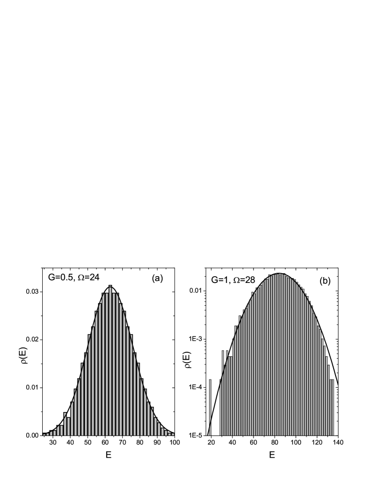
Figure 5: Density of states as a function of energy is shown by the histogram. The solid curve indicates the Gaussian distribution with the parameters determined by Eqs. (40) and (42). Both panels refer to half-occupied systems. Panel (a) for the 12-level system with $G=0.5$ displays an overall good Gaussian fit while the deviations are more clear in panel (b) where the density of states is plotted in the log scale for a larger system with stronger pairing, $G=1$. Here the effect of negative skewness is visible, as well as the presence of the gap.

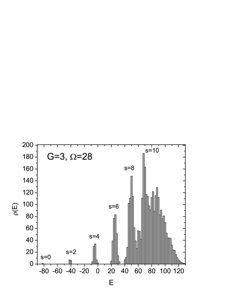
Figure 6: Density of states in the half-occupied system with $\Omega=28$ and pairing strength $G=3.$ The strong pairing dominates single-particle structure resulting in the peaks of the level density that correspond to the quasispin families of the degenerate model.

6.3 Quasiparticle temperature

As was discussed in detail in [19, 65], there is no unique definition of temperature in a self-sustaining isolated mesoscopic system. Complementary to the thermodynamic (microcanonical) definition of the previous subsection, we can find the effective value of temperature for each individual many-body state by fitting the occupation numbers found in the EP solution to those given by the thermal ensemble, Eq. (39). We can refer to this assignment as a measurement with the aid of the quasiparticle thermometer, and denote the resulting temperature as ${\cal T}\,.$

The correspondence between excitation energy and quasiparticle temperature ${\cal T}\,$ for each eigenstate in the 12-level model is presented in Fig. 7. The scattered points clearly display a regular trend to thermalization in agreement with the hyperbolas predicted by Eq. (45). Although thermodynamic and quasiparticle temperature are well correlated, Fig. 8, their numerical scales are different, $T\approx 2.5{\cal T}.$ Furthermore, the concept of quasiparticle thermalization is meaningful only for relatively weak pairing, where large fluctuations due to the proximity of the phase transition are present. The quality of thermalization deteriorates as stronger pairing makes the dynamics more and more regular. The inability of the strongly paired system to fully thermalize dynamics was demonstrated earlier [56]. The role of non-pairing interactions is essential for equilibration. But the failure of the single-particle thermometer to reflect correctly the spectral evolution in the limit of very strong interaction is a general feature [19, 65].

Figure 7: Excitation energy and quasiparticle temperature ${\cal T}$ of individual states in the half-occupied, 12-level ladder model. The solid line shows the energy-temperature relation from Eq. (45), assuming scaling $T\approx 2.5{\cal T}.$

Figure 8: Comparison of thermodynamic and quasiparticle temperatures for the half-occupied, 12-level ladder model. Three panels correspond to pairing strengths $G=$0.5, 0.7 and 1.0, from left to right, respectively. The regular trends in scattered points confirm approximate thermalization with temperature ratio $T\approx 2.5{\cal T}.$ The agreement deteriorates for stronger pairing.

6.4 Pairing phase transition

In Fig. 9 the pairing gap is plotted as a function of quasiparticle temperature. The gap was calculated using Eq. (38) with the quasiparticle temperature substituting the BCS external temperature parameter. This makes the consideration consistent with the occupancies given by Eqs. (36) and (39). The half-occupied, 12-level ladder model was again used for this example. The choice of a larger system not only results in the increased number of $s=0$ states, but, more importantly, reduces the particle number fluctuations that can disrupt the fitting procedure, especially in the pairing phase transition region.

Fig. 9 demonstrates the phase transition from the paired state at lower temperature (or excitation energy) to a normal state at a higher temperature. Few low-lying states have a considerable pairing gap, whereas the gap disappears in the sufficiently excited states. The invariant entropy [67] can be an alternative method for visualizing the phase transition [56, 68]. This quantity is basis-independent and reflects the sensitivity of a particular eigenstate to the changes of a parameter of the many-body Hamiltonian, here the pairing strength $G$. The peak in the invariant entropy points out the location of the pairing phase transition as a function of $G$ and excitation energy $E$ of a particular state. However, it is important to notice that the phase transition pattern is strongly influenced [19, 65] by other parts of residual interaction.

Figure 9: Pairing gap as a function of quasiparticle temperature in the 12-level model with pairing strength $V$=0.5 and 0.7 for left and right panels, respectively.

7 New theoretical perspectives

7.1 Hartree-Fock approximation based on the exact pairing solution

Instead of the normal Fermi-occupation picture with a Slater determinant as a trial many-body function for the mean field approximation, the EP solution with its specific single-particle occupancies provides a new starting point for the consistent consideration of other parts of the residual interaction. In this subsection we illustrate this point with the help of Belyaev’s [69] pairing plus quadrupole (P+Q) model Hamiltonian for a single-$j$ level,

$$H=-G\,L^{\dagger}L-\frac{\chi}{2}\sum_{\kappa}{\cal M}^{\dagger}_{2\,\kappa}{\cal M}_{2\,\kappa}\,,$$ (46)

where the multipole operators are defined as

$${\cal M}_{K\,\kappa}=\,\sum_{m_{1}m_{2}}\,(-)^{j-m_{1}}\left(\begin{array}[]{ccc}j&K&j\\ -m_{1}&\kappa&m_{2}\end{array}\right)\,a^{\dagger}_{2}a_{1}\,.$$ (47)

Only the ratio $\chi/G$ of the strength of quadrupole-quadrupole interaction to the pairing strength is important since the energy scale can be fixed so that $G=1.$

In the pure pairing limit, $\chi=0$, the degenerate pairing model is recovered with the ground state energy $(\Omega=2j+1)$

$$E=G\frac{N}{4}(\Omega-N+2).$$ (48)

Pairing correlation energy in the BCS with constant pairing is given by $\Delta^{2}/G\,.$ For the exact solution we define the correlation energy as the ground state expectation value of the pairing part of the Hamiltonian with the monopole contribution subtracted. In the degenerate case

$$E_{\rm corr}=G\frac{N}{4}(\Omega-N).$$ (49)

The opposite limit with no pairing can be treated by making a transition to a deformed mean field in the Hartree approximation [70]. For axially symmetric deformation, the expectation value of the quadrupole moment is

$$\langle{\cal M}_{2\,0}\rangle=\sum_{m}\frac{2[3m^{2}-j(j+1)]}{\sqrt{\Omega(\Omega^{2}-1)(\Omega^{2}-4)}}\,n_{m}\,,$$ (50)

in terms of the occupation numbers $n_{m}=\langle a^{\dagger}_{m}\,a_{m}\,\rangle$ in the intrinsic frame with the $z$-axis oriented along the symmetry axis. In this case

$$\langle{\cal M}_{2\,-2}\rangle=\langle{\cal M}_{2\,2}\rangle=0.$$ (51)

The deformed single-particle energies in the body-fixed frame can be obtained via the usual self-consistency requirement,

$$\epsilon_{m}=-\chi\,\frac{2[3m^{2}-j(j+1)]}{\sqrt{\Omega(\Omega^{2}-1)(\Omega^{2}-2)}}\,\langle{\cal M}_{2\,0}\rangle\,.$$ (52)

The energy minimum for an even-$N$ system corresponds to the Fermi occupation of the $N/2$ lowest pairwise degenerate orbitals $|m|=1/2,3/2,\dots(N-1)/2$ for prolate, or $|m|=j,j-1,\dots j-(N-2)/2$ for oblate shape. The corresponding quadrupole moment is then given by

$$\langle{\cal M}_{2\,0}\rangle=-\frac{1}{2}\,\frac{N(\Omega^{2}-N^{2})}{\sqrt{\Omega(\Omega^{2}-1)(\Omega^{2}-4)}}$$ (53)

for prolate deformation and

$$\langle{\cal M}_{2\,0}\rangle=\frac{1}{2}\,\frac{N(2\Omega-N)(\Omega-N)}{\sqrt{\Omega(\Omega^{2}-1)(\Omega^{2}-4)}}$$ (54)

for oblate deformation. Deformation energy is quadratic in $\langle{\cal M}_{2\,0}\rangle$, so that the oblate deformation is preferred for $N<\Omega/2$ and the prolate one for $N>\Omega/2.$

The full problem is driven by the competition between pairing and deformation. While deformation tends to split the single particle energies (Nilsson orbitals), Eq. (52), the pairing can resist such a shape transition by creating a particle distribution unfavorable for deformation. In the single-$j$ model these effects have been discussed by Baranger [70] with the help of the BCS and the Hartree approximation. However, as demonstrated earlier, the BCS may be unreliable in the transitional region. The use of the projected HFB and the resulting improvement against traditional HFB for a similar single-$j$ model have been recently discussed in [71]. Our goal here is to supplement the Hartree treatment with the exact pairing solution.

Similar to the Hartree+BCS approach in [70] we look for a self-consistent solution, where the occupation numbers in the deformed basis agree with the exact solution to the pairing problem [72]. Prior to calculations, one can estimate the ratio $\chi/G$ corresponding to the BCS phase transition. Assuming for example an oblate shape with $N\leq\Omega/2$ we have the Fermi energy at $m=j-(N-2)/2$ with the density of single-particle states approximately found as $\nu_{{\rm F}}=2/(\epsilon_{m-1}-\epsilon_{m})$, that for a half-occupied system leads to

$$(\chi/G)_{\rm crit}\approx 3.6\,\Omega.$$ (55)

In Fig. 10 we present the results for a model with $j=19/2$, The particle number, $N=8$, was selected to avoid an exactly half-occupied shell when particle-hole symmetry and oblate to prolate shape change lead to special features that are of no interest for our goal. For this model the transition from spherical to deformed shape takes place at $\chi/G\approx 70$, Eq. (55). The pairing correlation energy shown in Fig. 10(a) as a function of $\chi/G$ starts near $\chi/G=0$ with a value prescribed by the degenerate model. As the relative strength of the quadrupole-quadrupole interaction increases, the deformation inhibits pairing. However, in Fig. 10(a) we see a key difference between the BCS and exact treatment. Within the BCS the pairing correlation energy goes to zero quite sharply once the system becomes deformed. In contrast, the exact solution finds that pairing correlations decay very slowly and extend far into the deformed region. In panel 10(b) the expectation value of $\langle{\cal M}_{20}\rangle$ is shown as a function of $\chi/G$. In the pairing limit $\chi/G\rightarrow 0$ the deformation is zero whereas in the deformed limit the value $\langle{\cal M}_{20}\rangle$ is expressed via Eq. (54) or (53). Here again the exact treatment produces a softened and extended phase transition.

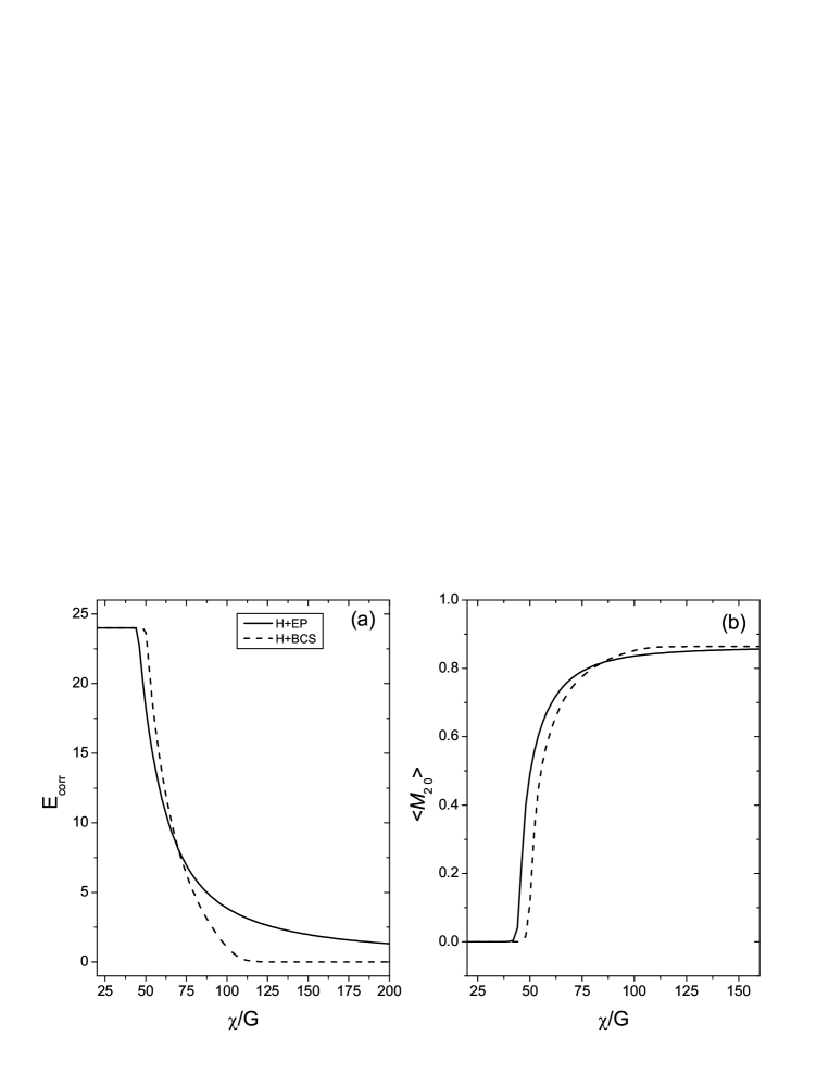
Figure 10: Comparison of pairing correlation energy, panel (a), and quadrupole deformation, panel (b), for Hartree+BCS and Hartree+EP treatments of the P+Q model for a single-$j$ level, $j=19/2$, and $N=8$ particles. For pairing correlation energy $G=1.0\,$ is assumed.

The Hartree approximation ignores another important effect relevant to our consideration, namely, the contribution of the exchange terms to the pairing channel. This contribution is particularly strong in small systems and leads to an additional enhancement of the pairing strength $G\rightarrow G+2\chi/\Omega^{2}$ [73]. The results of Hartree-Fock + EP calculations that include this additional term are shown in Fig. 11. Due to the exchange term, pairing correlations never disappear. Presence of pairing correlations in a pure quadrupole-quadrupole Hamiltonian is also confirmed by an exact solution in the full shell model diagonalization [73]. The BCS treatment, however, fails to reproduce this effect.

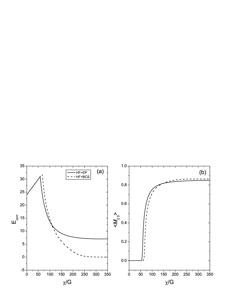
Figure 11: Comparison of pairing correlation energy and quadrupole deformation; in contrast to Fig. 10, the exchange contribution from the quadrupole-quadrupole interaction to the pairing channel is included.

7.2 New Random Phase Approximation

Here we show how the RPA-like approximation can be developed starting from the exact solution of the pairing problem. There are two main types of the RPA used in the literature (and a variety of close approaches distinguished by the details of the formalism), the RPA based on the vacuum of noninteracting particles or that of the BCS, or HFB, quasiparticles (the so-called QRPA). We will try to describe collective vibrations generated by the residual interaction on top of the exact ground state of the pairing problem. The formalism of the generalized density matrix [74, 75] seems to be suitable for this purpose.

The generalized density matrix (GDM) is the set of the operators

$$R_{12}=a^{\dagger}_{2}a_{1}$$ (56)

acting in the full Hilbert space of a many-body system; this set at the same time forms a matrix labeled by single-particle subscripts (1,2). We do not perform any canonical transformation to the quasiparticle operators and therefore work invariably within a system of a certain particle number. The one-body observables as operators in many-body space are traces of the GDM operator over single-particle indices,

$$Q=\sum_{a}q_{a}\quad\Rightarrow\quad Q=\sum_{12}q_{12}a^{\dagger}_{1}a_{2}={\rm Tr}\,(qR).$$ (57)

With the Hamiltonian of the system taken as a sum of independent particle energies in the mean field, $\epsilon_{1}$, and the general residual two-body interaction $V_{12;34}$, the exact operator equations of motion for the GDM can be symbolically written as

$$[R,H]=[S,R],$$ (58)

where $S$ is the generalized self-consistent field operator (a linear functional of the GDM),

$$S=\epsilon+W\{R\},\quad W_{14}\{R\}=\sum_{23}V_{12;34}R_{32},$$ (59)

and the interaction matrix elements are antisymmetrized.

Now we assume that the Hamiltonian contains the pairing part (1) as well as other residual interactions, $H=H_{p}+H^{\prime}$. Correspondingly we can put

$$R=R^{\circ}+R^{\prime},\quad W=W^{\circ}+W^{\prime},\quad W^{\circ}=W\{R^{\circ}\},\quad W^{\prime}=W\{R^{\prime}\}.$$ (60)

The assumption of the exact solution of the pairing problem means that we found the occupancies, $R^{\circ}$, and the pairing potential, $W^{\circ}$, satisfying

$$[R^{\circ},H_{p}]=[\epsilon+W^{\circ},R^{\circ}].$$ (61)

This stage of the solution provides the states $|s,a\rangle$ with seniority $s$ and energy $E_{sa}$, where $a$ numbers the states within the subset of certain seniority; if needed we also can explicitly indicate rotational quantum numbers $J_{a}$ and $M_{a}$. The remaining part $R^{\prime}$ of the GDM should satisfy

$$[R^{\prime},H_{p}]+[R^{\circ},H^{\prime}]+[R^{\prime},H^{\prime}]=[W^{\prime},R^{\circ}]+[\epsilon+W^{\circ},R^{\prime}]+[W^{\prime},R^{\prime}].$$ (62)

The commutators in such expressions are to be understood as, for example

$$[W^{\prime},R^{\prime}]_{12}=\sum_{3}(W^{\prime}_{13}R^{\prime}_{32}-R^{\prime}_{13}W^{\prime}_{32}).$$ (63)

This is the point where we can make RPA-like approximations.

For definiteness, we consider the transitions from the paired states $s=0,J=0$ to the states with $s=2,J\neq 0$ in the next sector. We are looking for a collective mode that is related to such excitations. This means that there exist states, in our case coherent combinations of excited states with certain $J$, that have large off-diagonal matrix elements of excitation by a one-body multipole operator from the ground state. The latter can be in turn renormalized by the collective mode. Let us characterize this branch of the spectrum with the help of collective coordinates $\alpha$ and conjugate momenta $\pi$ (we omit in this symbolic derivation their quantum numbers of angular momentum and its projection). These variables are Hermitian quantum operators that satisfy the commutation relation $[\alpha,\pi]=i$ so that no procedure of subsequent requantization is needed. The collective Hamiltonian of the mode can be written as

$$H^{\prime}=\frac{1}{2}C\alpha^{2}+\frac{1}{2B}\pi^{2}+\,\dots,$$ (64)

where the scalar contraction of the tensor operators is implied and the dots include high order anharmonic terms important for the soft mode [76, 77].

We are looking for the operator solution of Eq. (62) in the form of the expansion in collective operators $\alpha$ and $\pi$,

$$R^{\prime}_{12}=r^{(10)}_{12}\alpha+r^{(01)}_{12}\pi+\,\dots,$$ (65)

and

$$W^{\prime}_{12}=w^{(10)}_{12}\alpha+w^{(01)}_{12}\pi+\,\dots,$$ (66)

where the superscripts $(n,m)$ refer to the component containing $n$ collective coordinate and $m$ collective momenta operators. The dots again denote the higher order parts, $n+m>1$, symmetrized in due way [76, 77]. The collective operators producing the transition in many-body space are written explicitly whereas the coefficients $r^{(nm)}_{12}$ and $w^{(nm)}_{12}$ are the $c$-numbers to be found as single-particle amplitudes of the coherent superposition that forms a collective mode. The operator expansion (65, 66) does not assume the smallness of anharmonic effects - we merely decompose the problem in various operator structures. In the present context we limit ourselves by the harmonic part although it can be used [76, 77] for the situations of strong anharmonicity as well.

The operator $R$, by definition (56), has seniority selection rules $|\Delta s|=2$. We take in the operator equation (62) matrix elements $\langle 0|c\rangle$ between the ground state $|0\rangle$ and the collective state $|c\rangle$ in the adjacent sector $s=2$ with angular momentum corresponding to that of collective operators $\alpha$ and $\pi$. Now we evaluate the matrix elements of various terms in Eq. (62) aiming at the segregation of terms linear in $\alpha$ and $\pi$. The first term in the right hand side gives, according to Eq. (65),

$$[R^{\prime}_{12},H_{p}]=(\bar{E}^{\circ}_{c}-\bar{E}^{\circ}_{0})(r^{(10)}_{12}\alpha+r^{(01)}_{12}\pi).$$ (67)

Here the barred energies are the centroids of the energy distribution of the actual ground state and the one-phonon state in the sectors $s=0$ and $s=2$, respectively. The second term in eq. (62) does not have required matrix elements whereas in the commutator $[R^{\prime},H^{\prime}]$ we need to perform commutation explicitly using the assumed form of the collective operators (65-67),

$$[R^{\prime}_{12},H^{\prime}]=\frac{i}{B}r^{(10)}_{12}\pi-iCr^{(01)}_{12}\alpha.$$ (68)

The situation with the terms $[W^{\circ},R^{\prime}]$ and $[W^{\prime},R^{\circ}]$ is more complicated. Within each sector of given $s$, the pairing solution GDM $R^{\circ}$ has not only diagonal but also off-diagonal elements between the eigenstates of $H_{p}$. As shown in Figs. 2 and 3, very few pair-vibrational states have significant off-diagonal matrix elements of this type. For our illustrative purposes, here we neglect the off-diagonal terms within a given sector and take into account only diagonal elements of $R^{\circ}$ and $W^{\circ}$. The neglected contributions correspond to the anharmonic admixtures of pair vibrations to multipole modes and can be easily included in the consideration. Because of the specific character of the monopole pairing interaction, the matrix elements of $R^{\circ}$ and $W^{\circ}$ are diagonal over single-particle subscripts as well. Higher order structures in the collective Hamiltonian and in the GDM, as well as terms generated by the commutator $[W^{\prime},R^{\prime}]$ do not contribute to matrix elements linear in $\alpha$ and $\pi$ and with the selection rule $\Delta s=2$. But, similarly to Eq. (67), the commutators with $R^{\circ}$ and $W^{\circ}$ bring in the differences of the single-particle occupancies and pairing potentials averaged over the states contributing to the collective mode.

As a result, we come to the coupled equations for the coordinate and momentum RPA amplitudes (these contributions can be distinguished by their behavior under time-reversal operation in the sector with $J\neq 0$):

$$r^{(10)}_{12}\Omega_{12}-iCr^{01}_{12}=[\bar{n}_{2}(c)-\bar{n}_{1}(0)]w^{10}_{12},$$ (69)

$$r^{01}_{12}\Omega_{12}+\frac{i}{B}r^{10}_{12}=[\bar{n}_{2}(c)-\bar{n}_{1}(0)]w^{01}_{12}.$$ (70)

Here the generalized frequencies are introduced,

$$\Omega_{12}=\bar{E}^{\circ}_{0}-\bar{E}^{\circ}_{0}+\epsilon_{2}-\epsilon_{1}+\bar{W}^{\circ}_{c}-\bar{W}^{\circ}_{0}.$$ (71)

This set of equations leads to a formal solution, analogous to that in the conventional RPA,

$$r^{10}_{12}=\frac{[\bar{n}_{2}(c)-\bar{n}_{1}(0)]}{\Omega^{2}_{12}-\omega^{2}}(\Omega_{12}w^{10}_{12}+iCw^{01}_{12}),$$ (72)

$$r^{01}_{12}=\frac{[\bar{n}_{2}(c)-\bar{n}_{1}(0)]}{\Omega^{2}_{12}-\omega^{2}}(\Omega_{12}w^{01}_{12}+\frac{i}{B}w^{10}_{12}),$$ (73)

where the unknown collective frequency is $\omega=(C/B)^{1/2}$.

The collective elements of the GDM are to be found from the integral equations (72) and (73) with the specific choice of the residual interaction self-consistently generating the field $W^{\prime}$, Eq. (60). This can be done explicitly in the case of the factorizable multipole-multipole force; the frequency $\omega$ and correct normalization of the mode are also obtained in this process similarly to the standard procedure in terms of the barred quantities. Having at our disposal the phonon amplitudes $r^{(10)}_{12}$ and $r^{(01)}_{12}$, we can self-consistently find the barred quantities averaged over the collective wave functions. This procedure, that reminds the thermal RPA built on the equilibrium density matrix but with occupation numbers and mean-field corrections defined by the interaction rather than by an external heat bath, can be performed in an iterative manner. The cranking description for the deformed nucleus can be also reformulated in the same spirit; it is interesting to note that the pure EP solution predicts [56] an yrast-line with the moment of inertia close to the rigid body value.

8 Conclusion

The pioneering work by Belyaev [8] carried out a detailed analysis of pairing phenomena in nuclei. Applying the BCS techniques in the nuclear shell model environment, he demonstrated the effects of pairing on various nuclear properties, including the ground state structure, single-particle transitions, collective vibrations, onset of deformations and rotations. It was shown that the Cooper phenomenon in systems with a discrete single-particle spectrum does require, in contrast to large systems, a certain strength of the pairing interaction. The drawbacks of the BCS approximation, related to the particle number violation and the sharp disappearance of pairing correlations at the phase transition point, were also pointed out.

The development started with Belyaev’s work and supported by similar studies [78, 79] was continued through the next forty years. Now the pairing problem is well and alive being one of the main chapters of modern nuclear physics and mesoscopic physics in general. The interest in pairing is constantly revived by the accumulation of data and especially by the advances towards nuclei from stability where the pairing is a key tool that determines the binding of a system and its response to the excitation. At this point it becomes increasingly important to get rid of the shortcomings of the BCS approximation and unify the description of the structure and reactions.

We presented a way of solving the pairing problem essentially along the lines similar to that of Belyaev’s paper, substituting the BCS approximation by the exact solution simplified by the seniority symmetry. As a magnifying glass, this solution reveals and fixes the weak points of the standard approach. We saw the importance of the exact treatment for the ground state, low-lying excitations, coupling through the continuum, and spectroscopic factors associated with single-particle removal and pair emission (transfer) reactions. We could also discuss on the new basis the global properties of the spectrum, thermalization and the phase transition region. In many cases, this exact treatment of pairing is practically simpler than solving the BCS equations with necessary corrections.

Certainly, the pairing problem is only a part of the physics of strongly interacting self-sustaining systems. Other interactions, with their own coherent and chaotic features, should be included in the consideration. We gave preliminary answers to the questions of further approximations necessary for the cases when the full problem does not allow for a complete solution. New generalizations of the mean field approach and random phase approximations can be developed on the background of the exactly found paired state. The interplay of pairing and other residual interactions can be an exciting and practically important topic of future studies.

The inspiring influence of Belyaev’s ideas is gratefully acknowledged by the authors who belong to the first and third generation of his pupils. The work was supported by the NSF grant PHY-0070911 and by the U. S. Department of Energy, Nuclear Physics Division, under contract No. W-31-109-ENG-38.

References

- [1] A. Bohr and B.R. Mottelson, Nuclear Structure, vol. 1 (Benjamin, New York, 1969).
- [2] M.G. Mayer and J.H.D. Jensen, Elementary Theory of Nuclear Shell Structure (Wiley, New York, 1955).
- [3] G. Racah, Phys. Rev. 63, 367 (1943).
- [4] G. Racah, I. Talmi, Phys. Rev. 89, 913 (1953).
- [5] B.R. Judd, Operator Techniques in Atomic Spectroscopy, (Princeton University Press, 1998).
- [6] J. Bardeen, L.N. Cooper and J.R. Schrieffer, Phys. Rev. 106, 162; 108, 1175 (1957).
- [7] A. Bohr, B.R. Mottelson and D. Pines, Phys. Rev. 110, 936 (1958).
- [8] S.T. Belyaev, Mat. Fys. Medd. Dan. Vid. Selsk. 31, No. 11 (1959).
- [9] A.L. Goodman, Adv. Nucl. Phys. 11, 263 (1979).
- [10] N.N. Bogoliubov, JETP 34, 58 (1958); Physica 26, 1 (1960).
- [11] H.J. Lipkin, Ann. Phys. 31, 528 (1960).
- [12] Y. Nogami, Phys. Rev. B 134, 313 (1964); Y. Nogami and I.J. Zucker, Nucl. Phys. 60, 203 (1964).
- [13] W. Satula and R. Wyss, Nucl. Phys. A676, 120 (2000).
- [14] J.A. Sheikh and P. Ring, Nucl. Phys. A665, 71 (2000).
- [15] G. Do Dang and A. Klein, Phys. Rev. 143, 735 (1966).
- [16] J. Bang and J. Krumlinde, Nucl. Phys. A141, 18 (1970).
- [17] F. Andreozzi, A. Covello, A. Gargano, L.J. Ye, A. and Porrino, Phys. Rev. C 21, 1094 (1980); Phys. Rev. C 32, 293 (1985).
- [18] K. Hagino and G.F. Bertsch, Nucl. Phys. A679, 163 (2000).
- [19] V. Zelevinsky, B. A. Brown, N. Frazier, and M. Horoi, Phys. Rep. 276, 85 (1996).
- [20] N. Giovanardi, F. Barranco, R.A. Broglia, and E. Vigezzi, Phys. Rev. C 65, 041304 (2002).
- [21] K. Bennaceur, J. Dobaczewski, and M. Ploszajczak, Phys. Rev. C 60, 034308 (1999).
- [22] A. Poves and A.P. Zuker, Phys. Rep. 70, 235 (1981).
- [23] B.A. Brown and B.H. Wildenthal, Ann. Rev. Nucl. Part. Sci. 38, 29 (1988).
- [24] W. A. Richter, M. G. van der Merwe, R. E. Julies and B. A. Brown, Nucl. Phys. A523, 325 (1991).
- [25] B. Wildenthal, Prog. Part. Nucl. Phys. 11, 5 (1984).
- [26] Y. Alhassid, D.J. Dean, S.E. Koonin, G. Lang, and W.E. Ormand, Phys. Rev. Lett. 72, 613 (1994).
- [27] M. Honma, T. Mizusaki, and T. Otsuka, Phys. Rev. Lett. 77, 3315 (1996).
- [28] M. Horoi, A. Volya, and V. Zelevinsky, Phys. Rev. Lett. 82, 2064 (1999).
- [29] A. Volya, B.A. Brown and V. Zelevinsky, Phys. Lett. B 509, 37 (2001).
- [30] H. Chen, T. Song and D.J. Rowe, Nucl. Phys. A582, 181 (1995).
- [31] Yang Yi and Xu Gong-ou, Phys. Rev. C 43, 1225 (1991).
- [32] D. J. Rowe, Nuclear Collective Motion, Models and Theory (Methuen and Co. Ltd., London, 1970).
- [33] R. A. Broglia, J. Terasaki, and N. Giovanardi, Phys. Rep. 335, 1 (2000).
- [34] P. Ring and P. Schuck, The Nuclear Many-Body Problem (Springer-Verlag, New York, 1980).
- [35] G. Do Dang and A. Klein, Phys. Rev. 143, 735 (1966); 147, 689 (1966).
- [36] G. Do Dang, R. M. Dreizler, A. Klein and C. Wu, Phys. Rev. 172, 1022 (1968).
- [37] A. Volya and V. Zelevinsky, Preprint MSUCL-1144 (1999).
- [38] J. Högaasen-Feldman, Nucl. Phys. 28, 258 (1961).
- [39] O. Johns, Nucl. Phys. A154, 65 (1970).
- [40] K. Hagino and G.F. Bertsch, Nucl. Phys. A679, 163 (2000).
- [41] D. J. Rowe, Rev. Mod. Phys. 40, 153 (1968).
- [42] J. Dukelsky and P. Schuck, Nucl. Phys. A512, 466 (1990); Phys. Lett. B 387, 233 (1996).
- [43] F. Krmpotic, E.J.V. de Passos, D.S. Delion, J. Dukelsky, and P. Schuck, Nucl. Phys. A637, 295 (1998).
- [44] R.W. Richardson, Phys. Lett. 3, 277 (1963); Phys. Lett. 5, 82 (1963); Phys. Lett. 14, 325 (1965); J. Math. Phys. 6, 1034 (1965); J. Math. Phys. 18, 1802 (1977). Phys. Rev. 141, 949 (1966); Phys. Rev. 144, 874 (1966); Phys. Rev. 159, 792 (1967).
- [45] R. W. Richardson and N. Sherman, Nucl. Phys. 52, 221 (1964).
- [46] J. Dukelsky, C. Esebbag, and S. Pittel, Phys. Rev. Lett. 88, 062501 (2002).
- [47] F.J. Dyson, J. Math. Phys. 3, 166 (1962).
- [48] Feng Pan, J. P. Draayer, and W. E. Ormand, Phys. Lett. B 422, 1 (1998).
- [49] Feng Pan, J. P. Draayer, and Lu Guo, J. Phys. A 33, 1597 (2000).
- [50] J. Dukelsky and P. Schuck, LANL preprint cond-mat/0009057.
- [51] O. Burglin and N. Rowley, Nucl. Phys. A602, 21 (1996).
- [52] H. Molique and J. Dudek, Phys. Rev. C 56, 1795 (1997).
- [53] A.K. Kerman, R.D. Lawson, and M.H. Macfalane, Phys. Rev. 124, 162 (1961).
- [54] N. Auerbach, Nucl. Phys. 76, 321 (1966).
- [55] A. Holt, T. Engeland, M. Hjorth-Jensen, and E. Osnes, Nucl. Phys. A634, 41 (1998).
- [56] A. Volya, V. Zelevinsky, and B. A. Brown, Phys. Rev. C 65, 054312 (2002).
- [57] N. Frazier, B.A. Brown, and V. Zelevinsky, Phys. Rev. C 54, 1665 (1996).
- [58] V. Zelevinsky, Yad. Fiz. 65, 1220 (2002).
- [59] M. Horoi, B.A. Brown, and V. Zelevinsky, Phys. Rev. C 65, 027303 (2002).
- [60] V. Zelevinsky and A. Volya, in Challenges of Nuclear Structure, ed. A. Covello (World Scientific, Singapore, 2002) p. 261.
- [61] M. Horoi, B.A. Brown, and V. Zelevinsky, Phys. Rev. C, in press.
- [62] C. Mahaux and H.A. Weidenmüller, Shell-Model Approach to Nuclear Reactions (North Holland, Amsterdam, 1969).
- [63] V.V. Sokolov and V.G. Zelevinsky, Nucl. Phys. A504, 562 (1989).
- [64] A. Volya and V. Zelevinsky, nucl-th/0211039 (2002).
- [65] V. Zelevinsky, Ann. Rev. Nucl. Part. Sci. 46, 237 (1996).
- [66] N. Dinh Dang and V. Zelevinsky, Phys. Rev. C 64, 064319 (2001).
- [67] V.V. Sokolov, B.A. Brown, and V. Zelevinsky, Phys. Rev. E 58, 56 (1998).
- [68] P. Cejnar, V. Zelevinsky, and V.V. Sokolov. Phys. Rev. E 63, 036127 (2001).
- [69] S.T. Belyaev, Sov. Phys. JETP 12, 968 (1961).
- [70] M. Baranger, K. Kumar, Nucl. Phys 62, 113 (1965).
- [71] J.A. Sheikh, P. Ring, E. Lopes, and R. Rossignoli, Phys.Rev. C 66, 044318 (2002).
- [72] A. Volya, B. A. Brown, and V. Zelevinsky, Progr. Theor. Phys. Suppl. 146, 636 (2002).
- [73] A. Volya, Phys. Rev. C 65, 044311 (2002).
- [74] S.T. Belyaev and V.G. Zelevinsky, Yad. Fiz. 16, 1195 (1973).
- [75] V.G. Zelevinsky, Progr. Theor. Phys. Suppl. 74-75, 251 (1983).
- [76] V. Zelevinsky and A. Volya, in Perspectives of Nuclear Structure and Nuclear Reactions (Dubna, 2002) p. 101.
- [77] V. Zelevinsky, in Mapping the Triangle, AIP Conf. Proc., vol. 638 (Melville, New York, 2002) p. 155.
- [78] V.G. Soloviev, Nucl. Phys. 9, 655 (1958/59); Mat. Fys. Dan. Vid. Selsk. 1, No. 11 (1961).
- [79] A.B. Migdal, Nucl. Phys. 13, 655 (1959).