Abstract

The Unitary Correlation Operator Method (UCOM) is applied to realistic potentials. The effects of tensor correlations are investigated. The resulting phase shift equivalent correlated interactions are used in the no-core shell model for light nuclei and for mean-field calculations in the Fermionic Molecular Dynamics model for nuclei up to mass $A=48$.

1 Motivation

In principle the interaction among hadrons should be derived from Quantum Chromo Dynamics (QCD), the fundamental theory of the strong interaction. However a description of the atomic nucleus in terms of QCD is still not in sight. Therefore one starts with so called realistic nucleon-nucleon (NN) potentials that reproduce phase shifts up to $E_{lab}=300\mathrm{MeV}$ and the deuteron properties. This procedure is not unique as the NN-interaction is momentum dependent. Furthermore, exact calculations of the three- and four-nucleon system show that realistic NN-potentials are not sufficient and genuine three-body forces are needed to describe the binding energies.

Our aim is to use realistic NN-potentials in nuclear structure calculations where the many-body Hilbert space is spanned by Slater determinants. Although those form in principle a complete basis they are very badly suited to describe the correlations induced by the repulsive core and the strong tensor part in the NN-potential $\!\hbox{}\mathop{\vphantom{V}\smash{V}}\limits_{\!\sim}\hbox{}\!$. A large scale shell model calculation with the bare interaction for ${}^{3}\mathrm{He}$ needs already $50\>\hbar\Omega$ excitations, a Hilbert space of dimension $10^{5}$, to achieve convergence.

2 Unitary Correlation Operator Method (UCOM)

In order to avoid the large off-diagonal matrix elements that scatter to high lying shell-model states we propose [1-2] to first perform a unitary transformation of the Hamiltonian

$$\!\hbox{}\mathop{\vphantom{\hat{H}}\smash{\hat{H}}}\limits_{\!\sim}\hbox{}\!={{\!\hbox{}\mathop{\vphantom{C}\smash{C}}\limits_{\!\sim}\hbox{}\!}}^{{\dagger}}(\!\hbox{}\mathop{\vphantom{T}\smash{T}}\limits_{\!\sim}\hbox{}\!+\!\hbox{}\mathop{\vphantom{V}\smash{V}}\limits_{\!\sim}\hbox{}\!)\!\hbox{}\mathop{\vphantom{C}\smash{C}}\limits_{\!\sim}\hbox{}\!=\!\hbox{}\mathop{\vphantom{T}\smash{T}}\limits_{\!\sim}\hbox{}\!+\!\hbox{}\mathop{\vphantom{\hat{H}}\smash{\hat{H}}}\limits_{\!\sim}\!{}^{[2]}+\!\hbox{}\mathop{\vphantom{\hat{H}}\smash{\hat{H}}}\limits_{\!\sim}\!{}^{[3]}+\cdots$$ (1)

that incorporates the effects of the repulsive and tensor correlations in the sense of a pre-diagonalization. In Eq. (1) $\!\hbox{}\mathop{\vphantom{T}\smash{T}}\limits_{\!\sim}\hbox{}\!$ denotes the kinetic energy, $\!\hbox{}\mathop{\vphantom{\hat{H}}\smash{\hat{H}}}\limits_{\!\sim}\!{}^{[2]}$ the two-body, and $\!\hbox{}\mathop{\vphantom{\hat{H}}\smash{\hat{H}}}\limits_{\!\sim}\!{}^{[3]}$ the three-body part of the correlated Hamiltonian. With this unitary transformation the original eigenvalue problem in terms of the bare Hamiltonian $\!\hbox{}\mathop{\vphantom{H}\smash{H}}\limits_{\!\sim}\hbox{}\!$ and many-body states $\big{|}\,{\hat{\Psi}_{n}}\,\big{>}$ that include short ranged correlations can be rewritten in terms of a correlated Hamiltonian $\!\hbox{}\mathop{\vphantom{\hat{H}}\smash{\hat{H}}}\limits_{\!\sim}\hbox{}\!$ and more simple states $\big{|}\,{\Psi_{n}}\,\big{>}$ that are Slater determinants or superpositions of a limited number of those:

$$\!\hbox{}\mathop{\vphantom{H}\smash{H}}\limits_{\!\sim}\hbox{}\!\big{|}\,{\hat{\Psi}_{n}}\,\big{>}=E_{n}\big{|}\,{\hat{\Psi}_{n}}\,\big{>}\quad\rightarrow\quad\!\hbox{}\mathop{\vphantom{\hat{H}}\smash{\hat{H}}}\limits_{\!\sim}\hbox{}\!\big{|}\,{\Psi_{n}}\,\big{>}={{\!\hbox{}\mathop{\vphantom{C}\smash{C}}\limits_{\!\sim}\hbox{}\!}}^{{\dagger}}\!\hbox{}\mathop{\vphantom{H}\smash{H}}\limits_{\!\sim}\hbox{}\!\!\hbox{}\mathop{\vphantom{C}\smash{C}}\limits_{\!\sim}\hbox{}\!\big{|}\,{\Psi_{n}}\,\big{>}=E_{n}\big{|}\,{\Psi_{n}}\,\big{>}$$ (2)

The correlator $\!\hbox{}\mathop{\vphantom{C}\smash{C}}\limits_{\!\sim}\hbox{}\!=\!\hbox{}\mathop{\vphantom{C}\smash{C}}\limits_{\!\sim}\!{}_{\Omega}\!\hbox{}\mathop{\vphantom{C}\smash{C}}\limits_{\!\sim}\!{}_{r}$ consists of the unitary radial correlator

$$\!\hbox{}\mathop{\vphantom{C}\smash{C}}\limits_{\!\sim}\!{}_{r}=\exp\biggl{\{}-i\sum_{i<j}\frac{1}{2}\Bigl{(}s(\!\hbox{}\mathop{\vphantom{r}\smash{r}}\limits_{\!\sim}\!{}_{ij})\,\!\hbox{}\mathop{\vphantom{p}\smash{p}}\limits_{\!\sim}\!{}_{rij}+h.a.\Bigr{)}\biggr{\}}$$ (3)

and the unitary tensor correlator

$$\!\hbox{}\mathop{\vphantom{C}\smash{C}}\limits_{\!\sim}\!{}_{\Omega}=\exp\biggl{\{}-i\sum_{i<j}\frac{3}{2}\vartheta(\!\hbox{}\mathop{\vphantom{r}\smash{r}}\limits_{\!\sim}\!{}_{ij})\>\Bigl{(}(\!\hbox{}\mathop{\vphantom{\vec{\sigma}}\smash{\vec{\sigma}}}\limits_{\!\sim}\!{}_{i}\,\!\hbox{}\mathop{\vphantom{\vec{r}}\smash{\vec{r}}}\limits_{\!\sim}\!{}_{ij})(\!\hbox{}\mathop{\vphantom{\vec{\sigma}}\smash{\vec{\sigma}}}\limits_{\!\sim}\!{}_{j}\,\!\hbox{}\mathop{\vphantom{\vec{p}}\smash{\vec{p}}}\limits_{\!\sim}\!{}_{\Omega ij})+h.a.\Bigr{)}\biggr{\}}\;.$$ (4)

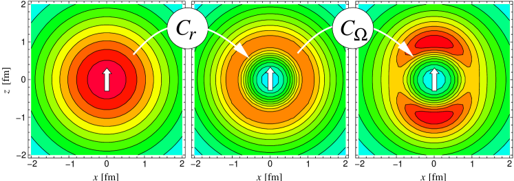
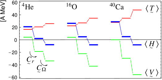
Figure 1: Upper part: two-body density $\rho^{(2)}_{S,T}(\vec{r}_{1}\!\!-\!\vec{r}_{2})$ of ${}^{4}\mathrm{He}$ for a pair of nucleons with isospin $T\!=\!0$ and parallel spins, $S\!=\!1,M_{S}\!=\!1$. Arrow indicates spin direction and $(x,y,z)=(\vec{r}_{1}\!\!-\!\vec{r}_{2})$ relative distance vector. Lower part: corresponding kinetic, potential and total energies per particle of ${}^{4}\mathrm{He}$, ${}^{16}\mathrm{O}$ and ${}^{40}\mathrm{Ca}$, without, with radial, and with radial and tensor correlations (Bonn-A).

When applied to a many-body state $\big{|}\,{\Psi}\,\big{>}$ the radial correlator $\!\hbox{}\mathop{\vphantom{C}\smash{C}}\limits_{\!\sim}\!{}_{r}$ shifts all particle pairs $(i,j)$ radially away from each other whenever they are too close, i.e. inside the range of the repulsive core. The strength function $s(r_{ij})$ controls the amount of the radial shift and is optimized to the potential under consideration. $\!\hbox{}\mathop{\vphantom{p}\smash{p}}\limits_{\!\sim}\!{}_{rij}$ is the radial component of the relative momentum. The effect of the transformation $\big{|}\,{\Psi}\,\big{>}\rightarrow\!\hbox{}\mathop{\vphantom{C}\smash{C}}\limits_{\!\sim}\!{}_{r}\big{|}\,{\Psi}\,\big{>}$ is shown in the upper part of Fig. 1 where the two-body density $\rho^{(2)}_{S,T}$ is displayed as a function of the distance vector $(\vec{r}_{1}\!-\!\vec{r}_{2})$ between two nucleons in ${}^{4}\mathrm{He}$. The $\rho^{(2)}_{S,T}$ on the l.h.s. is calculated with the shell-model state $\big{|}\,{(1s_{1/2})^{4}}\,\big{>}$ that is just a product of 4 Gaussians. It has a maximum at zero distance which is in contradiction to the short ranged repulsion of the interaction. This inconsistency is removed by the action of the radial correlator $\!\hbox{}\mathop{\vphantom{C}\smash{C}}\limits_{\!\sim}\!{}_{r}$ that moves density out of the region where the potential is repulsive. The corresponding kinetic, potential and total energies are displayed in the lower part of the figure for three nuclei. The radially correlated kinetic energy $\big{<}\,{\!\hbox{}\mathop{\vphantom{C}\smash{C}}\limits_{\!\sim}\!{}_{r}^{\dagger}\!\hbox{}\mathop{\vphantom{T}\smash{T}}\limits_{\!\sim}\hbox{}\!\!\hbox{}\mathop{\vphantom{C}\smash{C}}\limits_{\!\sim}\!{}_{r}}\,\big{>}$ increases somewhat compared to $\big{<}\,{\!\hbox{}\mathop{\vphantom{T}\smash{T}}\limits_{\!\sim}\hbox{}\!}\,\big{>}$ but this is overcompensated by the gain of about $-25\>\mathrm{MeV}$ per particle in the correlated potential energy. Nevertheless the nuclei are still unbound.

The tensor correlations are induced by $\!\hbox{}\mathop{\vphantom{C}\smash{C}}\limits_{\!\sim}\!{}_{\Omega}$ where the tensor operator in the exponent (Eq. (4)) creates shifts perpendicular to $\vec{r}_{ij}$. The amount of the displacement depends on the spin directions $\!\hbox{}\mathop{\vphantom{\vec{\sigma}}\smash{\vec{\sigma}}}\limits_{\!\sim}\!{}_{i}$ and $\!\hbox{}\mathop{\vphantom{\vec{\sigma}}\smash{\vec{\sigma}}}\limits_{\!\sim}\!{}_{j}$ of the particles relative to their distance vector. The operator $\!\hbox{}\mathop{\vphantom{\vec{p}}\smash{\vec{p}}}\limits_{\!\sim}\!{}_{\Omega ij}=\!\hbox{}\mathop{\vphantom{\vec{p}}\smash{\vec{p}}}\limits_{\!\sim}\!{}_{ij}-\!\hbox{}\mathop{\vphantom{\vec{p}}\smash{\vec{p}}}\limits_{\!\sim}\!{}_{rij}$, called orbital relative momentum, is the component of $\!\hbox{}\mathop{\vphantom{\vec{p}}\smash{\vec{p}}}\limits_{\!\sim}\!{}_{ij}$ perpendicular to $\!\hbox{}\mathop{\vphantom{\vec{r}}\smash{\vec{r}}}\limits_{\!\sim}\!{}_{ij}$. The overall strength of the tensor correlations is controlled by $\vartheta(r_{\!ij})$ and allows, for example, to map a purely $l\!=\!0$ deuteron wave function onto the exact one which includes an $l\!=\!2$ component and thus all tensor correlations [1]. The application of the tensor correlator $\!\hbox{}\mathop{\vphantom{C}\smash{C}}\limits_{\!\sim}\!{}_{\Omega}$ leads to the two-body density depicted in the right hand contour plot of Fig. 1. One may visualize the action of $\!\hbox{}\mathop{\vphantom{C}\smash{C}}\limits_{\!\sim}\!{}_{\Omega}$ as a displacement of probability density from the ’equator’ to both ’poles’, where the spin of the $S\!=\!1$ component of the nucleon pair defines the ’south-north’ direction. Again this costs kinetic energy but now the many-body state is in accord with the tensor interaction and one gains the binding needed to end up with about -8 MeV per particle, see lower part of Fig. 1.

3 Choice of correlation functions

Like the interaction the correlators are decomposed into the four spin isospin channels $S\!=\!0,1;\ T\!=\!0,1$ and the corresponding strength functions $s(r)$ and $\vartheta(r)$ are adjusted separately. As the repulsion is of short range the optimal radial shift functions can be found by minimizing the energy with respect to $s(r)$ in the corresponding channel. The result depends only weakly on the choice of the system, a constant trial state in the two-body system gives practically the same $s(r)$ as minimizing the energy of the deuteron or ${}^{4}\mathrm{He}$.

Figure 2: Strength of tensor correlation as function of particle distance.

Unlike the repulsive core the tensor part of the interaction, that is due to pion exchange, is of long range. Therefore, adjusting $\vartheta(r)$ by mapping a pure $l\!=\!0$ trial state for the deuteron to the exact eigenstate leads to the very long ranged tensor correlator strength $\vartheta^{d}(r)$ shown in Fig. 2. When used in systems with more than two particles this correlator is not useful as it induces large three- and more-body parts in the correlated interaction ($\!\hbox{}\mathop{\vphantom{\hat{H}}\smash{\hat{H}}}\limits_{\!\sim}\!{}^{[3]},\ldots$) that are very complicated to handle. Therefore we restrict the range of the tensor correlations and consider in the following the three $\vartheta(r)$ labeled by $\alpha$, $\beta$ and $\gamma$ shown in Fig. 2. With those we take care of the short range part of the tensor correlations. The long range part must then be described by the many-body state $\big{|}\,{\Psi}\,\big{>}$. The presence of the other particles will destroy at least partially the alignment of spins of a particle pair at larger distances (spin frustration) so that $\big{|}\,{\Psi}\,\big{>}$ can be again a rather simple many-body state.

4 Correlated interaction in momentum space

In Fig. 3 we display in momentum representation the matrix elements of the bare Argonne V8’ potential with those of the corresponding correlated interaction $\!\hbox{}\mathop{\vphantom{\hat{H}}\smash{\hat{H}}}\limits_{\!\sim}\!{}^{[2]}$. The left column is for the ${}^{1}S_{0}$ channel where due to $S\!=\!0$ only the radial correlator acts.

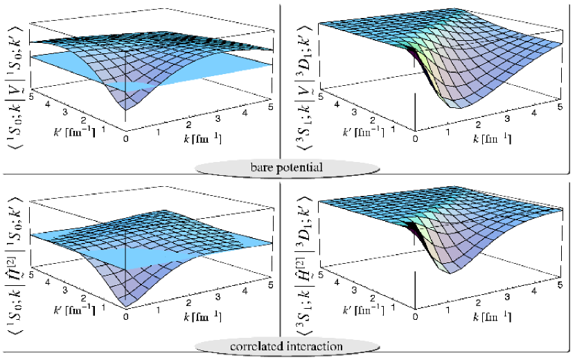
Figure 3: Matrix elements in momentum representation for the uncorrelated and correlated Argonne V8’ potential. Left: ${}^{1}S_{0}$ channel, plane denotes zero, vertical range from -2 to 2 $\mathrm{fm}^{-1}$. Right: tensor mixing between ${}^{3}S_{1}$ and ${}^{3}D_{1}$ channel, vertical range from -1.5 to 0 $\mathrm{fm}^{-1}$.

It is obvious that the goal of pre-diagonalization is achieved. Beyond momentum transfers of about 2 fm^-1 the off-diagonal matrix elements calculated with correlated states are close to zero. Our result is in good agreement with $V_{low-k}$ obtained with renormalization group methods [1,4]. In the right column the matrix elements between the $l\!=\!0$ and $l\!=\!2$ triplet channels are shown. Here only the tensor components of the interaction contribute. For the correlated state we use the correlation strength $\vartheta^{\alpha}(r)$ shown in Fig. 2. Despite the restricted range the correlator achieves a substantial reduction of the matrix elements. With the long ranged correlator $\vartheta^{d}(r)$ derived from the deuteron the off-diagonal matrix elements vanish completely.

5 No-core shell model calculations

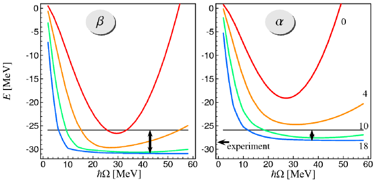
Figure 4: Ground state energy of ${}^{4}\mathrm{He}$ calculated with Argonne V8’ as function of harmonic oscillator parameter $\hbar\Omega$ and number of major shells included. L.h.s.: Hamiltonian correlated with tensor correlator of range $\beta$, r.h.s.: shorter range $\alpha$. Horizontal line: benchmark calculations [5].

In order to test the UCOM we use the correlated Hamiltonian in two-body approximation $\!\hbox{}\mathop{\vphantom{\hat{H}}\smash{\hat{H}}}\limits_{\!\sim}\!{}^{[2]}$ with the no-core shell model code of P. Navrátil [6] and compare with benchmark calculations for ${}^{4}\mathrm{He}$ [5].

In Fig. 4 we show the ground state energy as a function of the oscillator parameter for $0$, $4$, $10$ and $18\>\hbar\Omega$ excitations calculated with tensor correlators of range $\beta$ and $\alpha$. The correlated Hamiltonian obtained with the medium ranged correlator $\beta$ gives with a single Slater determinant ($0\>\hbar\Omega$) a minimum in energy at almost the exact energy (horizontal line). Admixing more and more configurations lowers the energy and convergence is reached at about $8\hbar\Omega$. One should keep in mind that the bare interaction needs many-body spaces that are orders of magnitude larger. For example at $\hbar\Omega=25\>\mathrm{MeV}$ the binding energy calculated with excitations up to $18\>\hbar\Omega$ included is only $-6\>\mathrm{MeV}$. If we use the short-ranged tensor correlator $\alpha$ the optimal single Slater determinant is $7\>\mathrm{MeV}$ above the exact eigenvalue. As can be seen in Fig. 4 convergence is not as fast but the overbinding is reduced to about $2\>\mathrm{MeV}$. This difference to the reference calculations is attributed to the missing contributions from $\!\hbox{}\mathop{\vphantom{\hat{H}}\smash{\hat{H}}}\limits_{\!\sim}\!{}^{[3]}$ and $\!\hbox{}\mathop{\vphantom{\hat{H}}\smash{\hat{H}}}\limits_{\!\sim}\!{}^{[4]}$.

6 Mean-field calculations in FMD basis

For heavier nuclei no-core shell model calculations are not feasible and we perform mean-field calculations in the framework of the Fermionic Molecular Dynamics (FMD) model [3]. The trial state in this approach consists of a single Slater determinant with single-particle states that are parametrized as a single or a sum of two Gaussians. As Hamiltonian we use the correlated Bonn-A interaction that is complemented by a momentum-dependent two-body correction term. This correction term has to simulate the effect of the missing three- and more-body terms of the correlated interaction and the effect of the genuine three-body forces. It is adjusted to reproduce the binding energies and radii of the doubly-magic nuclei ${}^{4}\mathrm{He}$, ${}^{16}\mathrm{O}$ and ${}^{40}\mathrm{Ca}$. Minimizing the binding energy with respect to the parameters of the single-particle states yields intrinsic states. The resulting one-body densities are shown for some nuclei in Fig. 5.

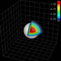
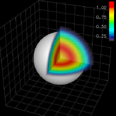
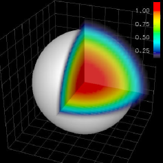
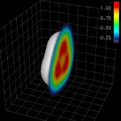
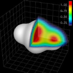
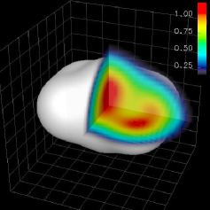
Figure 5: One-body densities of ${}^{4}\mathrm{He}$, ${}^{16}\mathrm{O}$, ${}^{40}\mathrm{Ca}$ and ${}^{12}\mathrm{C}$, ${}^{20}\mathrm{Ne}$, ${}^{24}\mathrm{Mg}$.

Besides the spherical nuclei ${}^{4}\mathrm{He}$, ${}^{16}\mathrm{O}$ and ${}^{40}\mathrm{Ca}$ we obtain also an axial ${}^{20}\mathrm{Ne}$ and a triaxial ${}^{24}\mathrm{Mg}$. The energies of the intrinsic states are shown in Fig. 6. For the $p$-shell we achieve a substantial improvement by using single-particle states with two Gaussians per nucleon. For the doubly-magic nuclei the spherical intrinsic states can be regarded as a good approximation of the ground states. On the other hand nuclei between closed shells are intrinsically deformed so that a projection on good angular momentum should be performed before comparing with experimental binding energies.

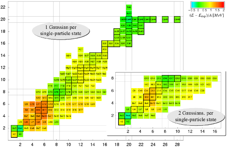
Figure 6: Deviation of intrinsic energies from experimental ground state energies. Insert: two Gaussians per single particle state.

Configuration mixing calculations taking into account rotations and vibrations are under way and should allow a description of the low lying spectra. First results are promising.

We are grateful to Petr Navrátil for providing his no-core shell model code used in the ${}^{4}\mathrm{He}$ calculations.

[1] T. Neff, H. Feldmeier, NPA713 (2003) 311
[2] H. Feldmeier et al., NPA632 (1998) 61
[3] H. Feldmeier, J. Schnack, Rev.Mod.Phys. 72 (2000) 655
[4] S. Bogner et al., nucl-th/0108041
[5] H. Kamada, et al., PRC64 (2001) 044001
[6] P. Navrátil et al., PRC61 (2000) 61044001