Quantum thermodynamic fluctuations of a chaotic Fermi–gas model

Abstract

We investigate the thermodynamics of a Fermi gas whose single–particle energy levels are given by the complex zeros of the Riemann zeta function. This is a model for a gas, and in particular for an atomic nucleus, with an underlying fully chaotic classical dynamics. The probability distributions of the quantum fluctuations of the grand potential and entropy of the gas are computed as a function of temperature and compared, with good agreement, with general predictions obtained from random matrix theory and periodic orbit theory (based on prime numbers). In each case the universal and non–universal regimes are identified.

1.  Laboratoire de Physique Théorique et Modèles Statistiques,
Bât. 100, Université de Paris-Sud, 91405 Orsay Cedex, France

2.  Department of Physics of Complex Systems, The Weizmann Institute of Science,
76100 Rehovot, Israel

PACS numbers: 21.60.-n, 24.60.Lz, 05.30.Fk, 05.45.Mt
Keywords: Fermi gas, statistical fluctuations.

1 Introduction

Fermi gases confined to small volumes present distinct finite size effects in their thermodynamic properties. Among the different corrections to the bulk behavior, some are smooth functions of the parameters of the system. They typically depend on geometric aspects of the volume occupied by the gas (e.g. surface and curvature terms). In contrast, other corrections are fluctuating functions. These quantum (or mesoscopic) fluctuations are related to the discreteness of the single–particle spectrum, and are sensitive to the nature of the dynamics of the particles in the gas. In many cases they are small compared to the bulk, but may play nevertheless an important role (like, for example, in nuclear physics where shell effects are crucial in the determination of the shape of atomic nuclei [1, 2]). In other (more spectacular) situations, they provide the dominant contribution. This occurs for example in the electronic orbital magnetism in quantum dots – where they can be larger than the Landau susceptibility [3, 4, 5] –, or in the persistent currents in mesoscopic rings [6, 7] – where the bulk contribution vanishes. In all cases the quantum fluctuations disappear when the temperature is raised.

Instead of a detailed computation and description of the quantum fluctuations for a particular system, the aim here is to study their statistical properties. The interest of such an analysis is well known: using a minimum amount of information, a statistical approach allows to establish a classification scheme among the fluctuations of different physical systems. It also allows to distinguish the generic from the specific, and provides a powerful predictive tool in complex systems. A general description of the statistical properties of the quantum fluctuations of thermodynamic functions of integrable and chaotic ballistic Fermi gases, and of their temperature dependence, was developed in Ref.[8].

From a classical point of view, there are two extreme cases of single–particle motion, namely integrable and fully chaotic. The case of a mixed phase space (e.g., coexistence of regular and chaotic motion) being the generic one. In all cases, in a Fermi gas model the quantum thermodynamic fluctuations can be directly related to the fluctuations of the single–particle, discrete, energy levels. Schematically, there are two distinct types of single–particle fluctuations. On the one hand there are the local fluctuations, i.e. those occurring on scales of the order of the single–particle mean level spacing $\delta$. For the two extreme dynamics mentioned above, these fluctuations are known to be universal [9], namely Poisson for integrable motion, random matrix in full chaos. The second type of fluctuations generically present in any single–particle spectrum are long range correlations, that occur on a scale $E_{c}$, where $E_{\rm c}$ is the energy associated with the shortest classical periodic orbit of the mean field (inverse time of flight across the system). In contrast to the local fluctuations, the long range modulations depend on the short–time specific properties of the dynamics and are therefore non–universal, either for integrable, mixed, or fully chaotic dynamics (thought their importance varies in each case).

Properties related to both types of single–particle fluctuations have been identified in the nuclear behavior. For example, shell effects in the nuclear masses are a clear manifestation of the long range correlations, whereas nearest–neighbor spacing statistics and the distribution of widths of neutron resonances illustrate universal local fluctuations. However, a global and comprehensive picture of the quantum fluctuations has not yet emerged. An important additional ingredient are certainly the variations in the nucleus of the nature of the dynamics as a function of the excitation energy. But even in the case of a scaling mean–field motion where the classical dynamics is energy independent (like when putting a Fermi gas inside a hard wall box or billiard) the physical behavior of the gas can be quite complex and rich, and both types of fluctuations (local and long range) can in fact manifest in different quantities related to the system, or in the same quantity at different temperatures [8].

One might think that a fully chaotic single–particle dynamics implies universal quantum fluctuations of the thermodynamics of the gas, well described by some random matrix model (Wigner, two–body random, etc). This belief is not true in general. The reason is that the thermodynamic fluctuations are universal only when they are controlled by the local single–particle fluctuations. And this is not always the case. For example, it has been shown, in particular, that the statistical properties of the ground–state energy of a many–body system are controlled by the short periodic orbits (at least in systems with a ground state well described by a mean–field approximation, like the atomic nucleus) [8]. The corresponding distribution is therefore non–universal. As a consequence, it makes no sense to model the ground–state fluctuations by some random matrix model, that possess no information on the specific mean–field short time properties of the dynamics.

Our purpose here is to illustrate the richness of the thermodynamic quantum fluctuations and to explicitly check some of the predictions by considering a particular example of a Fermi gas with a fully chaotic classical dynamics. The system considered is a mathematical model. It is achieved by considering a spectrum of single–particle energy levels constructed from the imaginary part of the complex zeros of the Riemann zeta function. The Fermi gas is obtained by filling the single–particle energy levels with an average occupation number determined by the Fermi–Dirac distribution. This model of a chaotic gas was introduced in Ref.[10], where general motivations as well as dynamical analogies were given. If this Fermi–gas model is viewed as an element of the periodic table, following nuclear physics terminology we referred to it as the Riemannium [10]. Aside its mathematical interest, physically the Riemannium is an important model because it possesses all the typical dynamical properties and characteristics of a realistic chaotic gas, while it greatly facilitates the numerical and analytical computations (e.g., all the ingredients required in a semiclassical description of its thermodynamic properties are known). This is quite unusual in fully chaotic systems, and therefore offers a rather unique model to test general results and ideas.

The basic quantities to be computed are the probability distributions, at a given temperature, of the quantum fluctuations of the grand potential and of the entropy of the gas. We consider a degenerate gas in the grand canonical ensemble; other ensembles (e.g., canonical) may be considered as well. In particular, it can be shown that to leading order in an expansion of large chemical potential, the fluctuations of the energy of the gas at a fixed number of particles coincide with those of the grand potential. Our results therefore apply to the total energy. In a semiclassical approximation, the fluctuations are described by the periodic orbits of the classical dynamics associated with the single–particle motion [11, 12, 2, 13]. In the Riemannium, the role of the periodic orbits is played by the prime numbers. The basic equations and the relevant energy scales of the Riemannium are introduced in §2. In §3 we analyze the fluctuations of the grand potential. The corresponding distribution is non–universal at all temperatures (including $T=0$, the case considered in [10]). The asymptotic moments of the distribution, obtained for a large chemical potential, are well reproduced by some convergent sums dominated by the smaller prime numbers (i.e., short periodic orbits). Odd moments are non–zero, implying an asymmetric distribution at all temperatures. At a finite chemical potential, large prime numbers introduce corrections to the asymptotic moments. These corrections to the non–universal leading–order behavior are, in contrast, universal, and described by random matrix theory.

The entropy fluctuations are studied in §4. Their character strongly depends on temperature. For a chaotic dynamics without time reversal symmetry, which corresponds to the Riemannium, these fluctuations present several remarkable features, predicted in [8]. For temperatures $T\ll\delta$, the variance of the entropy fluctuations increases linearly. In a second regime, when $\delta\ll T\ll E_{\rm c}$, the variance saturates to a constant value. This initial behavior of the variance (i.e. linear growth followed by a saturation), and more generally of the probability distribution of the entropy fluctuations, was predicted to be universal, namely identical for any chaotic system without time reversal symmetry (with a given single–particle mean level spacing at Fermi energy). It is well described by the fluctuations obtained from a GUE random matrix single–particle spectrum. The shape of the probability distribution strongly depends on temperature, and converges towards a Gaussian as temperature increases. However, this universal behavior disappears for temperatures of the order $E_{\rm c}$ or higher, where the statistical properties of the gas do not coincide any more with random matrix theory. The probability distribution of the fluctuations is now described by the short periodic orbits, which are system dependent. In this high temperature regime the typical size of the fluctuations shows an overall exponential decay. All these predictions are worked out explicitly for the Riemannium and compared with numerical simulations. We have found very good agreement between theory and numerical experiments in all the regimes.

Although only two particular thermodynamic functions are discussed, they illustrate all the rich possibilities that may be encountered in other functions. Similar methods apply to them.

2 Thermodynamic framework

In the grand canonical ensemble the equilibrium properties of a Fermi gas are defined by the grand potential

$$\Omega(\mu,T)=-T\int dE~{}\log[1+e^{(\mu-E)/T}]~{}\rho(E)\ ,$$ (2.1)

where $T$ is the temperature (we set Boltzmann’s constant $k_{B}=1$), $\mu$ the chemical potential, and

$$\rho(E)=\sum_{j}\delta(E-E_{j})$$ (2.2)

is the single–particle density of states. In the Riemannium, the single–particle energies are given by the imaginary part of the upper–half complex zeros $s=1/2+iE_{j}$ of the Riemann zeta function $\zeta(s)$, $E_{j}=14.1347,21.0220,25.0109,\ldots$ (the values used in all our numerical simulations were obtained from [14]). They are expressed in arbitrary units, which are also those of temperature (since $k_{B}=1$). From the grand potential, other thermodynamic functions can be computed. We are particularly interested in the behavior of the entropy of the gas,

$$S(\mu,T)=-\left(\frac{\partial\Omega}{\partial T}\right)_{\mu}\ .$$ (2.3)

The number of complex zeros with imaginary part less than $E$ is [15],

$$n(E)=1-\frac{1}{2\pi}E\log\pi-\frac{1}{\pi}Im\log\Gamma\left(\frac{1}{4}-i\frac{E}{2}\right)-\frac{1}{\pi}Im\log\zeta\left(\frac{1}{2}-i~{}E\right)\ .$$ (2.4)

Expanding the $\Gamma$ function and using the Euler product representation of $\zeta$ in the last term, this expression splits naturally into a smooth plus an oscillatory part, as in the semiclassical approximation in quantum systems. The density of zeros $\rho(E)=dn/dE$ is written $\rho(E)=\overline{\rho}(E)+\widetilde{\rho}(E)$, with

$$\overline{\rho}(E) = \frac{1}{2\pi}\log\left(\frac{E}{2\pi}\right)+{\cal O}(E^{-2})\ ,$$ (2.5)

$$\widetilde{\rho}(E) = -\frac{1}{\pi}\sum_{p}\sum_{r=1}^{\infty}\frac{\log p}{p^{r/2}}\cos(E~{}r~{}\log p)\ .$$ (2.6)

In the Riemannium, the first term corresponds therefore to the asymptotic average density of the single–particle energy levels. In the fluctuating part $\widetilde{\rho}$, the sum is made over the prime numbers $p$. The comparison of this equation with the semiclassical Gutzwiller trace formula for the spectral density of a dynamical system [12], $\widetilde{\rho}(E)=\sum_{{\rm p.o.}}A_{{\rm p.o.}}\cos(S_{{\rm p.o.}}(E)/\hbar)$ (the sum is over the classical periodic orbits), shows that each prime number may be interpreted as the label of an unstable primitive periodic orbit $p$ of a fully chaotic system without time reversal symmetry, of action $S_{p}=E\,\tau_{p}$, period $\tau_{p}=\log p$, Lyapounov stability $\lambda_{p}=1$, repetitions labeled by $r$, and $\hbar=1$ [16, 17]. Because of this mapping, in the following we often refer to the prime numbers as periodic orbits. Putting aside the issue of the very existence of a classical system whose quantum eigenvalues coincide with the imaginary part of the Riemann zeros, it is the formal analogy with the semiclassical theory of dynamical systems that makes the Riemann zeros in general, and the Riemannium in particular, interesting on a physical basis as a model to test general theories of quantum chaotic systems. Additional support for a dynamical interpretation comes from numerical simulations, that clearly indicate [14] that the sequence of the imaginary part of the Riemann zeros obeys the Bohigas–Giannoni–Schmit conjecture for chaotic systems without time–reversal symmetry [18, 9]: asymptotically, their statistics coincide with those of eigenvalues of the GUE ensemble of random matrices [19].

Replacing the decomposition (2.5)–(2.6) of the density of states into (2.1) leads to a corresponding decomposition of the grand potential. A similar decomposition for other thermodynamic functions is obtained by derivation. We are interested in the statistical properties of the fluctuating part of those functions, and in their temperature dependence. In the forthcoming analysis, the different relevant scales are the following.

• Largest scale: chemical potential $\mu$

• Intermediate scale: shortest periodic orbit

  $${\rm Energy:}\ E_{\rm c}=h/\tau_{\rm min}=2\pi/\log 2\approx 9.06472\ ,$$

  $${\rm Time:}\ \tau_{\rm min}=\log 2\ ,$$

  $${\rm Temperature:}\ T_{\rm c}=E_{\rm c}/2\pi^{2}\approx 0.459224\ .$$

• Smallest scale: single–particle mean level spacing

  $${\rm Energy:}\ \delta=1/\overline{\rho}=2\pi/\log(\mu/2\pi)\ ,$$

  $${\rm Time:}\ \tau_{\scriptscriptstyle H}=h/\delta=\log(\mu/2\pi)\ ,$$

  $${\rm Temperature:}\ T_{\delta}=\delta/2\pi^{2}=1/\pi\log(\mu/2\pi)\ .$$

The intermediate scale is related to the shortest periodic orbit (or time of flight across the system at energy $\mu$) which, according to the previous analogy, corresponds here to the period $\tau_{\rm min}=\log 2$ associated with the prime number 2. $E_{\rm c}$ defines the outer energy scale of oscillations in the density of states (cf Eq.(2.6)). Due to the independence of the periods with energy in the Riemann dynamics, this energy scale is a fixed number. In the definition of the mean level spacing $\delta$, we have used the asymptotic leading order approximation of the average density of states. $\tau_{\scriptscriptstyle H}$ is the so–called Heisenberg time. The $2\pi^{2}$ factor (approximately 20) that relates energies and temperatures is dictated by semiclassical arguments [8], and it has to be taken into account in numerical comparisons. A final important parameter is the ratio of $E_{\rm c}$ to $\delta$, which measures the number of single–particle states contained in a scale $E_{\rm c}$,

$$g=E_{\rm c}/\delta=\log(\mu/2\pi)/\log 2\ .$$

In the semiclassical limit $\mu\rightarrow\infty$, the three energy scales are well separated, $\delta\ll E_{\rm c}\ll\mu$, and $g\rightarrow\infty$.

3 The grand potential

Replacing $\rho(E)$ by $\overline{\rho}$ in Eq.(2.1), integrating by parts, and applying Sommerfeld’s approximation (valid when $T\ll\mu$), we obtain the usual thermodynamic relation

$$\overline{\Omega}(\mu,T)=\overline{\Omega}_{0}(\mu)-\frac{\pi^{2}}{6}~{}\overline{\rho}(\mu)T^{2}\ ,$$ (3.1)

where $\overline{\Omega}_{0}$ is the grand potential at zero temperature. For the Riemannium

$$\overline{\Omega}_{0}(E)=-\frac{E^{2}}{4\pi}\log\left(\frac{E}{2\pi}\right)+\frac{3}{8\pi}E^{2}-\frac{7}{8}E-\frac{\log E}{48\pi}+c+{\cal O}(E^{-2})\ .$$

Terms of order up to $E^{-2}$ in $\bar{\rho}$ have been included in the integration. The determination of the constant $c$ is of numerical importance when computing the fluctuations. From the work of Selberg on the function $S_{1}(t)$ [20] (which, up to an overall sign, coincides with the fluctuating part of the grand potential at zero temperature), we can extract its value

$$c=\frac{1}{\pi}\int_{1/2}^{\infty}\log\left|\zeta(x)\right|dx-\lim_{E\rightarrow\infty}\left\{\int_{0}^{E}\overline{n}(x)\ dx-\frac{E^{2}}{4\pi}\log\left(\frac{E}{2\pi}\right)+\frac{3}{8\pi}E^{2}-\frac{7}{8}E-\frac{\log E}{48\pi}\right\},$$

where $\overline{n}(x)$ is the exact smooth part of the counting function, computed from equation (2.4). Evaluating numerically the integrals, the value of the constant is found to be $c\approx 0.75575$.

Replacing $\rho(E)$ by (2.6) in Eq.(2.1), the oscillating part of the grand potential is

$$\widetilde{\Omega}(\mu,T)=-\frac{1}{\pi}\sum_{p}\sum_{r=1}^{\infty}\frac{\kappa(\pi\ T\ r\log p)}{r^{2}\ p^{r/2}\log p}\cos(\mu\ r\log p)\ .\\$$ (3.2)

The function

$$\kappa(x)=x/\sinh x$$

takes into account temperature effects [2], and cuts exponentially the contribution of large prime numbers. If $T>T_{\rm c}$, the contribution of each orbit, including the shortest one, is exponentially small.

Equation (3.2) is an oscillatory function of $\mu$ that describes the quantum fluctuations of the grand potential. To study their statistical properties we define the average

$$\langle f\rangle\equiv\frac{1}{\Delta\mu}\int_{\mu-\Delta\mu/2}^{\mu+\Delta\mu/2}f(\mu^{\prime})~{}d\mu^{\prime}\ ,$$ (3.3)

for any thermodynamic function $f(\mu)$ associated to the Riemannium. The size of the average window $\Delta\mu$ has to be much smaller than $\mu$ (in order to extract local properties), but large enough to contain a sufficient number of oscillations to make the statistical approach meaningful, i.e. $E_{\rm c}\ll\Delta\mu\ll\mu$.

3.1 Variance

The most basic feature of the probability distribution of the fluctuations is the variance. The average of the square of $\widetilde{\Omega}$ can be written as an integral [8]

$$\langle\widetilde{\Omega}^{2}\rangle(\mu,T)=\frac{1}{2\pi^{2}}\int_{0}^{\infty}d\tau~{}\frac{\kappa^{2}(\pi T\tau)}{\tau^{4}}~{}K(\tau)\ .$$ (3.4)

The function

$$K(\tau)=\left\langle\sum_{i,j}A_{i}A_{j}\cos[\mu(r_{i}\log p_{i}-r_{j}\log p_{j})]\delta(\tau-\bar{\tau})\right\rangle\ ,$$ (3.5)

is the form factor, i.e. the Fourier transform of the two–point correlation function of the single–particle spectrum; $A_{i}=\log p_{i}/p_{i}^{r_{i}/2}$, and $\bar{\tau}=(\tau_{p_{i}}+\tau_{p_{j}})/2$. This function is central in our analysis. In the semiclassical limit $g\rightarrow\infty$ it is conjectured to coincide with the GUE form factor

$$K_{GUE}(\tau)={\rm min}\{\tau,\tau_{\scriptscriptstyle H}\}\ .$$ (3.6)

If we naively replace in (3.4) $K(\tau)$ by $K_{GUE}(\tau)$, the integral diverges at $\tau\rightarrow 0$. This is because at finite $g$ random matrix theory provides a wrong description of the short–time behavior of the form factor. For low values of $\tau$ the diagonal terms in Eq.(3.5) should be used [21],

$$K_{D}(\tau)=\sum_{i}A_{i}^{2}\ \delta(\tau-\tau_{i})\ .$$ (3.7)

This shows that the form factor is non–universal at short times, and that $K(\tau)=0$ for $\tau<\tau_{\rm min}$. The form factor behaves like $K_{GUE}$ only for times larger than some $\tau_{*}$. The intermediate time $\tau_{*}$ satisfies $({\rm Re}\gamma)^{-1}<\tau_{*}<\tau_{\scriptscriptstyle H}$, where $\gamma$ is the classical resonance (eigenvalue of the Perron–Frobenius operator) with the smallest real part [22].

Since short times dominate the fluctuations of the grand potential, in the limit $\tau\rightarrow 0$ we use in (3.4) the diagonal approximation of the form factor, and neglect for the moment the contributions of longer times,

$$\langle\widetilde{\Omega}^{2}\rangle_{{\rm D}}=\frac{1}{2\pi^{2}}\sum_{p,r}\frac{\kappa^{2}(\pi T\ r\log p)}{r^{4}~{}p^{r}~{}\log^{2}p}\ .$$ (3.8)

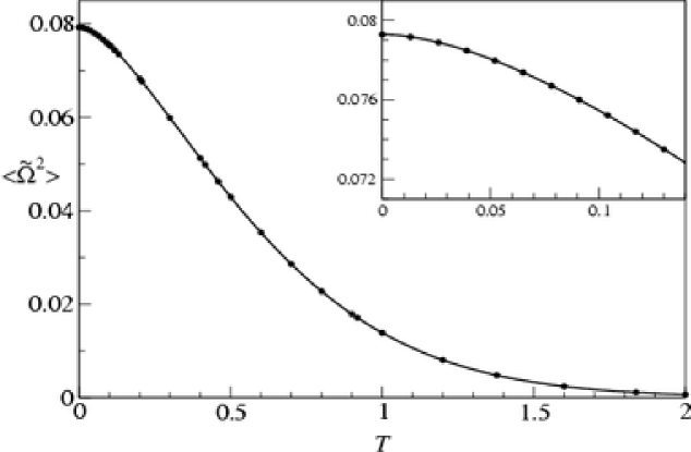
Figure 1: Variance of the grand potential fluctuations of the Riemannium as a function of temperature. Dots: numerical results computed in the chemical potential window $\mu=(267653402147\pm 6000)$ containing the zeros $(10^{12}+1940)$ to $(10^{12}+48684)$. Full line: theoretical prediction (3.8).

This is a convergent sum for all temperatures, and is independent of the chemical potential. At $T=0$ it gives the value $\langle\widetilde{\Omega}^{2}\rangle_{{\rm D}}\approx 0.079290$ [10]. Since the temperature factor is a monotonically decreasing function of $\tau$, the variance exponentially decreases with increasing temperature, and the role of the short orbits (small primes) in the fluctuations is further enhanced. Fig.1 compares Eq.(3.8) evaluated at different temperatures to numerical results obtained for the Riemannium (for reference, in the chemical potential window used to compute the fluctuations we have $T_{\delta}\approx 0.013$).

The agreement with the leading order description of the variance is excellent. However, as the chemical potential is lowered deviations from the asymptotic behavior are observed. The corrections may be obtained from Eq.(3.4), $\langle\widetilde{\Omega}^{2}\rangle=\langle\widetilde{\Omega}^{2}\rangle_{{\rm D}}+\langle\widetilde{\Omega}^{2}\rangle_{{\rm off}}$, by using the GUE form factor (3.6) for times $\tau>\tau_{*}$. This gives,

$$\langle\widetilde{\Omega}^{2}\rangle_{{\rm off}}=\frac{1}{2\pi^{2}}\int_{\tau_{\scriptscriptstyle H}}^{\infty}d\tau~{}\frac{(\tau_{\scriptscriptstyle H}-\tau)~{}\kappa^{2}(\pi T\tau)}{\tau^{4}}\ .$$ (3.9)

As temperature goes to zero, the temperature factor $\kappa^{2}$ tends to 1, and the integral is easily performed giving $\langle\widetilde{\Omega}^{2}\rangle_{{\rm off}}=-1/(12\pi^{2}\tau_{\scriptscriptstyle H}^{2})$. This provides a finite–$\mu$ correction to the variance, which decreases as $(\log\mu)^{-2}$. For increasing temperatures the correction is smaller. The off-diagonal terms thus provide a universal correction to the leading non universal diagonal term (namely, the only specific information on the system that enters the correction is the average density of states at Fermi energy, through $\tau_{\scriptscriptstyle H}=h\overline{\rho}$).

3.2 Higher moments and distribution

We already showed that to calculate the variance the diagonal approximation is accurate because the short orbits dominate the fluctuations. A generalization of the diagonal approximation allows to evaluate all the moments of the probability distribution of the grand potential by a method developed in [8] and [10]. The mechanism is an interference process between repetitions of primitive periodic orbits.

Defining the amplitude

$${\cal A}_{p,r}(T)=-\frac{1}{2\pi}\frac{\kappa(\pi\ T\ r\log p)}{r^{2}\ p^{r/2}\log p}\ ,$$ (3.10)

the third and fourth moments of the distribution of $\widetilde{\Omega}$ are found to be, in the diagonal approximation,

$$\langle\widetilde{\Omega}^{3}\rangle = 6~{}\sum_{p}\sum_{r_{1},r_{2}=1}^{\infty}{\cal A}_{p,r_{1}}~{}{\cal A}_{p,r_{2}}~{}{\cal A}_{p,r_{1}+r_{2}}\ ,$$ (3.11)

$$\langle\widetilde{\Omega}^{4}\rangle = 2~{}\sum_{p}\Big{[}~{}4\sum_{r_{1},r_{2},r_{3}=1}^{\infty}{\cal A}_{p,r_{1}}~{}{\cal A}_{p,r_{2}}~{}{\cal A}_{p,r_{3}}~{}{\cal A}_{p,r_{1}+r_{2}+r_{3}}-~{}6\sum_{r_{1},r_{2}=1}^{\infty}{\cal A}^{2}_{p,r_{1}}~{}{\cal A}^{2}_{p,r_{2}}$$ (3.12)

$$+~{}3\sum_{r_{1},r_{2}=1}^{\infty}\sum_{r_{3}=1}^{r_{1}+r_{2}-1}{\cal A}_{p,r_{1}}~{}{\cal A}_{p,r_{2}}~{}{\cal A}_{p,r_{3}}~{}{\cal A}_{p,r_{1}+r_{2}-r_{3}}\Big{]}+3~{}\langle\widetilde{\Omega}^{2}\rangle^{2}.$$

All the sums are convergent. We see explicitly that the third moment and the excess of the fourth moment (the term $3~{}\langle\widetilde{\Omega}^{2}\rangle^{2}$ being the fourth moment of a Gaussian distribution) are different from zero. The distribution of the fluctuations of the grand potential is therefore a non universal asymmetric function that strongly depends on the small prime numbers. It is displayed, for different temperatures, in Fig.2 [23].

Higher moments $k\geq 5$ may also be computed, with increasing complexity of the result. Corrections to the diagonal terms coming from off–diagonal contributions exist, but as already shown they are negligible in the limit $\mu\rightarrow\infty$. We thus ignore them.

These results are confirmed to high accuracy by the numerical data from the Riemann zeros (cf Fig.1 and Table 1).

4 The entropy

From Eq.(2.3) the entropy of the gas is expressed as,

$$S(\mu,T)=\int s\left(\frac{\mu-E}{T}\right)\rho(E)~{}dE=\sum_{j}s\left(\frac{\mu-E_{j}}{T}\right)\ ,$$ (4.1)

where

$$s(x)=\log(1+e^{x})-\frac{x}{1+e^{-x}}\ .$$ (4.2)

The function $s(x)$ is localized around $x=0$, and decays exponentially for $|x|\gg 1$. At very low temperatures ($T\ll T_{\delta}$), the function $S(\mu,T)$ has peaks as a function of $\mu$ centered at each single particle energy level (Riemann’s zero) of width $\ll\delta$. At these temperatures the entropy is therefore zero for $\mu\neq E_{j}$, and takes the value $\log 2$ when $\mu=E_{j}$. As the temperature increases, the width increases (while the height remains constant) and the peaks start to overlap. At temperatures $T\sim T_{\delta}$ and at a fixed $\mu$, only the energy levels distant by a few mean spacings from the chemical potential contribute to the entropy. The fluctuations are governed by the local statistics of the eigenvalues, which are universal (e.g., GUE). In this regime universality in the entropy fluctuations is expected. In contrast, at higher temperatures $T\stackrel{{\scriptstyle>}}{{\scriptstyle\sim}}T_{\rm c}$, when peaks separated from $\mu$ by a distance of order $E_{\rm c}$ start to contribute to the entropy, the universality will be lost because information on the scale of the shortest periodic orbit enters. We now substantiate this analysis by an explicit quantitative calculation.

Deriving with respect to temperature Eqs. (3.1) and (3.2), the smooth and fluctuating part of the entropy are given, respectively, by

$$\overline{S}(\mu,T) = \frac{\pi^{2}}{3}\ \overline{\rho}(\mu)\ T\ ,$$ (4.3)

$$\widetilde{S}(\mu,T) = \sum_{p}\sum_{r=1}^{\infty}\frac{\kappa^{\prime}(\pi\ T\ r\log p)}{r\ p^{r/2}}\cos(\mu\ r\log p)\ .$$ (4.4)

The function $\kappa^{\prime}(x)=d\kappa/dx$ decreases also exponentially for $x\gg 1$, producing a cut-off for prime numbers satisfying $\log p\gg 1/(\pi T)$. When $x\rightarrow 0$, $\kappa^{\prime}(x)$ vanishes linearly. The maximum of the function is located at $x\approx 1.6061$. Prime numbers that satisfy $r\log p\sim 1/(\pi T)$ give therefore the main contribution to the oscillations. At low temperatures large primes (long orbits) are selected. Smaller primes (e.g., short orbits) contribute as the temperature is raised.

4.1 Variance

Analogously to the grand potential, the variance of the entropy fluctuations may also be written in terms of the form factor,

$$\langle\widetilde{S}^{2}\rangle=\frac{1}{2}\int_{0}^{\infty}d\tau~{}\frac{\kappa^{\prime 2}(\pi\ T\ \tau)}{\tau^{2}}~{}K(\tau)\ .$$ (4.5)

We briefly review here the general results obtained in Ref.[8], and check them with the Riemannium.

The two different regimes of the form factor described in §3.1 split the integral (4.5) into three different parts,

$$\langle\widetilde{S}^{2}\rangle=\frac{1}{2}\left\{\sum_{r\log p<\tau_{*}}\frac{\kappa^{\prime 2}(\pi T\ r\log p)}{r^{2}~{}p^{r}}+\int_{\tau_{*}}^{\tau_{\scriptscriptstyle H}}d\tau~{}\frac{\kappa^{\prime 2}(\pi T\tau)}{\tau}+\tau_{\scriptscriptstyle H}\int_{\tau_{\scriptscriptstyle H}}^{\infty}d\tau~{}\frac{\kappa^{\prime 2}(\pi T\tau)}{\tau^{2}}\right\}\ .$$ (4.6)

The sum corresponds to the non universal short–time regime, whereas the two integrals correspond to the long–time random matrix behavior. These different terms dominate the integral at different temperatures.

* Low temperatures: $T\ll T_{\delta}$. In this regime the maximum of $\kappa^{\prime}$ is centered at times much larger than the Heisenberg time $\tau_{\scriptscriptstyle H}$. The dominant term in Eq.(4.6) is the last one. We can extend the integral down to zero with a negligible error. The variance of the entropy is

$$\langle\widetilde{S}^{2}\rangle\approx I_{2}\ \overline{\rho}(\mu)\ T=I_{2}\ T/\delta\ ,$$ (4.7)

where

$$I_{2}=\pi^{2}\int_{0}^{\infty}dx~{}\frac{\kappa^{\prime 2}(x)}{x^{2}}\approx 1.51836\ .$$ (4.8)

In this initial regime the growth is linear, with a slope proportional to the density of states. No additional specific information on the Riemann zeta is present in this formula. Eq.(4.7) reflects the discreteness of the single–particle spectrum, and is thus a very general result valid for arbitrary systems, independently of their dynamics [8]. The smooth part of the entropy grows also linearly with temperature, and is proportional to the density of states [24]. Compared to the mean value $\overline{S}$, the typical size of the fluctuations $\sqrt{\langle\widetilde{S}^{2}\rangle}$ are large (of order $(T/\delta)^{-1/2})$. In this regime the quantum fluctuations dominate.

* Intermediate temperatures: $T_{\delta}\ll T\ll T_{\rm c}$. Now the maximum of $\kappa^{\prime}$ is centered at times in between $\tau_{\rm min}$ and $\tau_{\scriptscriptstyle H}$. The dominant term in expression (4.6) is the second one, where we have introduced the GUE diagonal approximation of the form factor $K_{D}(\tau)=\tau$. Neglecting the contributions of short and long times we extrapolate the integral from 0 to $\infty$,

$$\langle\widetilde{S}^{2}\rangle\approx I_{1}=\frac{1}{2}\int_{0}^{\infty}dx~{}\frac{\kappa^{\prime 2}(x)}{x}\approx 0.0709159\ .$$ (4.9)

In this regime, the size of the entropy fluctuations are therefore insensitive to temperature variations, they saturate to a universal constant.

* High temperatures: $T\sim T_{\rm c}$ and higher. In this regime the diagonal approximation of the form factor is still accurate, but the short time (non universal) structure is now apparent. At this temperatures the entropy fluctuations are also sensitive to the fact that below $\tau_{\rm min}=\log 2$ the form factor is strictly zero. The dominant term in Eq.(4.6) is the first sum. The sum can be extended to all prime numbers and repetitions with negligible error, and gives a variance

$$\langle\widetilde{S}^{2}\rangle\approx\frac{1}{2}\sum_{p}\sum_{r=1}^{\infty}\frac{\kappa^{\prime 2}(\pi\ T\ r\log p)}{r^{2}\ p^{r}}\ .$$ (4.10)

For $T\gg T_{\rm c}$, all the terms of this sum are exponentially small, and the fluctuations vanish accordingly.

To have a global description of $\langle\widetilde{S}^{2}\rangle$ that interpolates between the different regimes described above a numerical evaluation of Eq.(4.6) is necessary. The result depends on $\mu$ through the Heisenberg time.

We have checked these predictions by a direct comparison of Eq.(4.6) to a numerical computation of the entropy variance as a function of temperature. The result is displayed in Fig.3 (for reference, $T_{\delta}\approx 0.013$). There is an excellent agreement with theory for all temperatures. The initial linear growth and the saturation to a plateau are amplified in the inset. The size of the fluctuations almost reaches the theoretical prediction (4.9) at $T\approx 2.5\ T_{\delta}\approx 0.03$. The expected intermediate plateau is however short, because the temperatures $T_{\delta}$ and $T_{\rm c}$ are not sufficiently well separated (due to the slow logarithmic decrease of $\delta$, even at these large values of $\mu$ we are not sufficiently asymptotic). The exponential decay is also well described.

4.2 Distribution

In the regime $T\ll T_{\rm c}$ the previous results confirm that the behavior of the statistical properties of the entropy fluctuations are universal. They depend only on the structure of the GUE form factor and not on any specific property of Riemann’s zeros. The universality is not expected to be valid only for the variance, but more generally for the full probability distribution. To check this, we compare the probability distribution of the entropy fluctuations obtained from Eq.(4.1) using two different single–particle spectra $\{E_{j}\}$:

• the zeros of the Riemann zeta function,

• the eigenvalues of a GUE ensemble of random matrices.

In the first case the probability distribution is computed by varying the chemical potential in a small window, whereas in the second by averaging over the Gaussian ensemble. Both probability distributions, computed at different temperatures, are plotted in Fig.4. At low temperatures both distributions are almost indistinguishable. Notice the strong sensitivity of the distribution to temperature variations. When temperatures of order $T_{\rm c}$ are reached (cf part d)), the universality is lost. For $T\sim T_{\rm c}$ the fluctuations are dominated by short orbits, and are system specific. The moments of the distribution can be computed by the same techniques used in §3.2 for the grand potential replacing ${\cal A}_{p,r}$ in Eq.(3.10) by ${\cal A}_{p,r}(T)=\kappa^{\prime}(\pi\ T\ r\log p)/(2r\ p^{r/2})$.

5 Concluding remarks

The use of the Riemannium as a test model in quantum mechanics is justified by two main reasons. First, by its genericity: the Riemann spectrum possesses all the generic features of a classically chaotic quantum system with no time reversal symmetry. Second, by its practical advantages, namely all the necessary quantum and semiclassical information required to work out accurate computations and comparisons is available. Hence, though this ”number theoretic” model may seem somewhat remote from a realistic system, it provides an excellent arena to verify the non trivial quantum mechanical properties of chaotic systems.

Based on semiclassical techniques and random matrix theory, several aspects of the thermodynamics of a chaotic Fermi gas have been verified. An accurate description of the probability distribution of the quantum fluctuations of the grand potential (or energy) and of the entropy of the Riemannium were obtained. In particular, the universal linear growth of the entropy variance followed by a saturation, with a further non universal exponential decay, were confirmed. The size of the saturation plateau, predicted in the regime $T_{\delta}\ll T\ll T_{\rm c}$, was relatively small (see the inset in Fig.3). This is due to the slow logarithmic asymptotic convergence properties of the Riemannium (in spite of the large chemical potential used in the numerical simulations, we are not very deep in the semiclassical limit. In fact, for the window analyzed in the figures the number of particles is around $10^{12}$, with $g\approx 35$. For an atomic nucleus or for electrons in a metallic grain, this value of $g$ corresponds to approximately $40\sim 50$ particles. In the Riemannium, in order to have $T_{\delta}$ and $T_{\rm c}$ separated by a factor of, say, 100, $\mu$ need to be of the order of $10^{30}$).

The high accuracy of the results obtained for all the quantities studied confirm the validity of the different approximations employed. The present theory therefore provides a solid ground to go beyond and test realistic systems. Of particular interest is the interplay between mean–field approximations, residual interactions and dynamics. Some encouraging results in this direction were already obtained in the study of nuclear masses [25].

This work has been supported by the European Commission under the Research Training Network MAQC (HPRN-CT-2000-00103) of the IHP Programme.

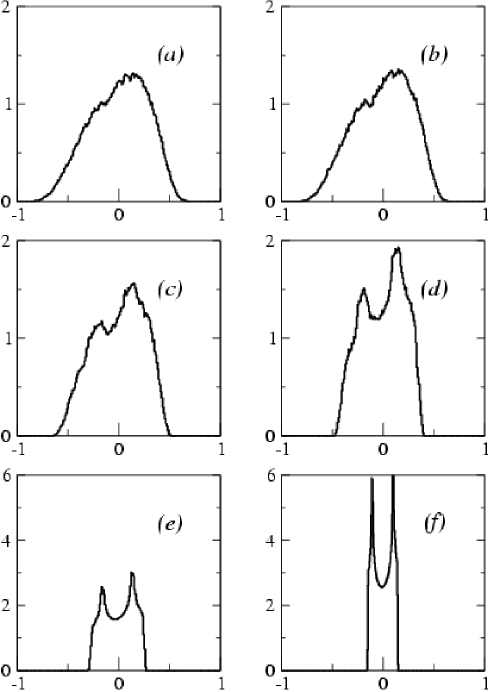
Figure 2: Normalized numerical histograms of the probability distribution of $\widetilde{\Omega}$ at different temperatures: (a) $T=0$, (b) $T=0.1$, (c) $T=0.3$, (d) $T=0.5$, (e) $T=0.8$, (f) $T=1.2$ (same chemical potential window as in Fig.1).

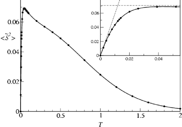
Figure 3: Variance of the entropy fluctuations of the Riemannium as a function of temperature. Dots: numerical results computed in the same chemical potential window as Fig.1. Full line: theoretical prediction (4.6). Dashed line (inset): low temperature approximation (4.7). Dot-dashed line (inset): saturation value (4.9).

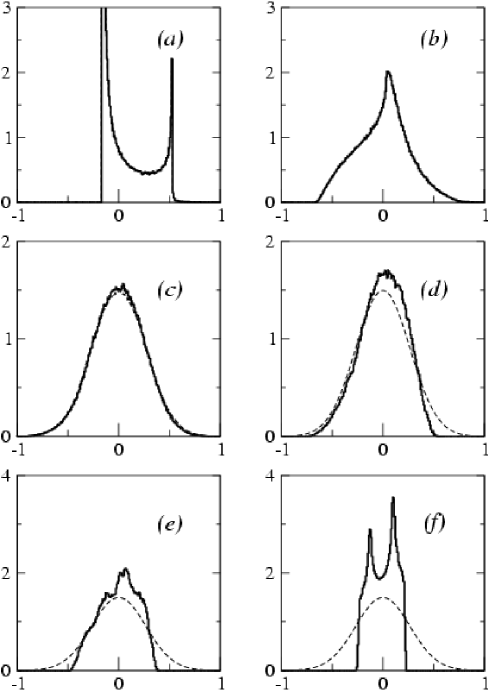
Figure 4: Normalized probability distribution of $\widetilde{S}$ at different temperatures. Full line: numerical results for the Riemannium computed in the same chemical potential window as Fig.1. Dash line: numerical results from a GUE single–particle spectrum. (a) $T=T_{\delta}\approx 0.013$, (b) $T=4\ T_{\delta}\approx 0.052$, (c) $T=0.1$, (d) $T=0.5$, (e) $T=0.8$, (f) $T=1.2$.

	T = 0	T = 0.3	T = 0.5
$\langle\widetilde{\Omega}^{2}\rangle$	$(7.928\pm 0.002)\times 10^{-2}$	$(5.9885\pm 0.0025)\times 10^{-2}$	$(4.2953\pm 0.0015)\times 10^{-2}$
	$7.9290\times 10^{-2}$	$5.9886\times 10^{-2}$	$4.2953\times 10^{-2}$
$\langle\widetilde{\Omega}^{3}\rangle$	$-(5.78\pm 0.02)\times 10^{-3}$	$-(3.44\pm 0.02)\times 10^{-3}$	$-(1.65\pm 0.01)\times 10^{-3}$
	$-5.7822\times 10^{-3}$	$-3.4377\times 10^{-3}$	$-1.6508\times 10^{-3}$
$\langle\widetilde{\Omega}^{4}\rangle$	$(1.480\pm 0.002)\times 10^{-2}$	$(7.625\pm 0.005)\times 10^{-3}$	$(3.586\pm 0.003)\times 10^{-3}$
	$1.4814\times 10^{-2}$	$7.6273\times 10^{-3}$	$3.5869\times 10^{-3}$

Table 1: Moments of $\widetilde{\Omega}$ at different temperatures. The upper values (with the errors) were obtained from the numerical distributions of figure (2.a), (2.c) and (2.d). The lower values are the semiclassical results (3.8), (3.11) and (3.12), respectively.

References

- [1] A. Bohr and B. R. Mottelson, Nuclear Structure, Benjamin, Reading, MS, 1969, Vol.I.
- [2] V. M. Strutinsky and A. G. Magner, Sov. J. Part. Nucl. 7 (1976) 138.
- [3] B. Shapiro, Waves Random Media 9 (1999) 271.
- [4] F. von Oppen, Phys. Rev. B 50 (1994) 17151.
- [5] K. Richter, D. Ullmo and R. Jalabert, Phys. Rep. 276 (1996) 1.
- [6] B. L. Altshuler, Y. Gefen, Y. Imry, Phys. Rev. Lett. 66 (1991) 88.
- [7] A. Schmid, Phys. Rev. Lett. 66 (1991) 80.
- [8] P. Leboeuf and A. G. Monastra, Ann. Phys. 297 (2002) 127.
- [9] O. Bohigas and M.-J. Giannoni, in Lecture Notes in Physics 209, (Springer, Berlin, 1984) p.1.
- [10] P. Leboeuf, A. G. Monastra and O. Bohigas, Reg. Chaot. Dyn. 6 (2001) 205.
- [11] R. Balian and C. Bloch, Ann. Phys. (N.Y.) 69 (1972) 76.
- [12] M. C. Gutzwiller, J. Math. Phys. 12, 343 (1971); Chaos in Classical and Quantum Mechanics (Springer–Verlag, New York, 1990).
- [13] M. Brack, Rev. Mod. Phys. 65 (1993) 677.
-
[14]
A. M. Odlyzko, “The -th zero of the
Riemann zeta function and million of its neighbors”, AT & T
Report, 1992 (unpublished); see also http://www.dtc.umn.edu/
~odlyzko/. - [15] H. M. Edwards, Riemann’s Zeta Function, New York, Academic Press, 1974.
- [16] M. V. Berry, in Quantum Chaos and Statistical Nuclear Physics edited by T. H. Seligman and H. Nishioka, Lectures Notes in Physics 263, (Springer Verlag, Berlin, 1986) p.1.
- [17] Three unusual features of the Riemann dynamics are the following: a) the independence of the periods with energy. This can be circumvented by interpreting the logarithm of the prime numbers as lengths, instead of periods; b) contrary to semiclassical approximations, the oscillating part is here exact (no correction terms are present) and, c) the negative sign in front of Eq.(2.6).
- [18] O. Bohigas, M.-J. Giannoni, and C. Schmit, Phys. Rev. Lett. 52 (1984) 1.
- [19] for the zeros of the Riemann zeta function, this conjecture is originally due to H. L. Montgomery, Proc. Symp. Pure Math. 24, 181 (1973); D. Goldston and H. L. Montgomery, Proceeding Conf. at Oklahoma State Univ. 1984, edited by A. C. Adolphson et al, p.183.
- [20] A. Selberg, Collected Papers, Vol. I, (Springer Verlag, Berlin, 1989) p.214.
- [21] M. V. Berry, Proc. Roy. Soc. Lond. A 400 (1985) 229.
- [22] O. Agam, J. Phys. I France 4 (1994) 697.
- [23] A further development of the technique allows to compute the tail of the distribution function, P. Bleher, O. Bohigas, P. Leboeuf and A. Monastra, to be published.
- [24] L. Landau and E. M. Lifchitz, Physique Statistique, Éditions Mir, Moscou, 1988.
- [25] O. Bohigas and P. Leboeuf, Phys. Rev. Lett. 88 (2002) 092502; Ibid 129903.