Radiative capture and electromagnetic dissociation involving loosely bound nuclei: the ⁸B example

Abstract

Electromagnetic processes in loosely bound nuclei are investigated using an analytical model. In particular, electromagnetic dissociation of ${{}^{8}}\mathrm{B}$ is studied and the results of our analytical model are compared to numerical calculations based on a three-body picture of the ${{}^{8}}\mathrm{B}$ bound state. The calculation of energy spectra is shown to be strongly model dependent. This is demonstrated by investigating the sensitivity to the rms intercluster distance, the few-body behavior, and the effects of final state interaction. In contrast, the fraction of the energy spectrum which can be attributed to E1 transitions is found to be almost model independent at small relative energies. This finding is of great importance for astrophysical applications as it provides us with a new tool to extract the E1 component from measured energy spectra. An additional, and independent, method is also proposed as it is demonstrated how two sets of experimental data, obtained with different beam energy and/or minimum impact parameter, can be used to extract the E1 component.

I Introduction

The properties of loosely bound nuclei have been studied in nuclear physics for a number of years. In particular some electromagnetic processes, such as certain charged particle capture reactions, are very interesting in themselves as they are of vital importance in astrophysical scenarios. Unfortunately, at stellar energies, the cross sections for these reactions are very small due to the Coulomb barrier and direct measurements are therefore extremely difficult. Instead one has to rely on theoretical extrapolations from experimentally accessible energies down to stellar ones. An alternative, indirect method to investigate radiative capture reactions, is to study electromagnetic dissociation (EMD) on heavy targets Baur and Rebel (1996). This technique gives an enormous increase in yield due to the huge amount of virtual photons produced by the high-$Z$ target, the more favorable phase space factor, and the possibility to use thicker targets. In principle it should therefore be possible to measure the cross section at very low relative energies. There are, however, also disadvantages with the indirect method; the most important being the admixture of $\gamma$-transitions with different multipolarities whereas the direct capture process, in most cases, should be completely dominated by E1 transitions. Since the cross sections for radiative capture and photo-dissociation are related via detailed balance for each separate multipole, it is necessary to have knowledge of the strengths of different multipole transitions in the EMD reaction.

The problem of extracting the E1 contribution from a measured EMD energy spectrum remains a challenge to the nuclear physics community. In Ref. Esbensen and Bertsch (1995) it was proposed to study the angular or momentum distributions of the breakup fragments. The idea was to employ the fact that interference terms, between E1 and E2 excitation amplitudes, will produce an asymmetry in these distributions. This method was, e.g., used in the analysis of ${{}^{8}}\mathrm{B}$ EMD Davids et al. (2001) where the E2 excitation amplitude, calculated within first-order perturbation theory, was renormalized in order to reproduce the asymmetry of the measured ${{}^{7}}\mathrm{Be}$ longitudinal momentum distribution. However, as was already noted in Ref. Esbensen and Bertsch (1995), the asymmetry due to E1-E2 interference strongly depends on the final state interaction (FSI) between the breakup fragments; or in other words, on the structure of the continuum up to relatively large energies. Moreover, terms which contribute to the asymmetry do not contribute to the integrated cross section from which the astrophysical $S$-factor is extracted. Finally, for low beam energies, higher-order dynamical effects will lead to a reduction of the asymmetry Esbensen and Bertsch (1996). Therefore we conclude that, if we are interested in astrophysical applications of EMD experiments, it is desirable to look for more stable, and less model dependent, characteristics than the asymmetries of angular and momentum distributions. In this paper we will present two novel methods to extract the E1/E2 ratio from EMD experiments.

We will use an analytical approach based on a two-cluster picture of the nucleus, but the effects of many-body structure will also be included. Our approach will be general in the sense that both neutron-rich and proton-rich systems can be studied. This model was first presented in Forssén et al. (2002a) while similar approaches also exist for one-neutron Bertulani and Baur (1988); Otsuka et al. (1994) and two-neutron Pushkin et al. (1996); Forssén et al. (2002b, c) halo nuclei. Although advanced numerical investigations are readily performed utilizing present day computer power, an analytical approach might have an advantage when exploring general physics features, and the sensitivity to different model assumptions.

The physics case which will be investigated throughout this paper is the ${{}^{8}}\mathrm{B}$ nucleus. The interest in ${{}^{8}}\mathrm{B}$ stems from its key role in the production of high-energy solar neutrinos. It is well-known that the probability for the reaction ${{}^{7}}\mathrm{Be}(p,\gamma){{}^{8}}\mathrm{B}$ at solar energies strongly depends on the structure of ${{}^{8}}\mathrm{B}$ and, in particular, on the asymptotics of the valence proton wave function (WF). This reaction has been studied indirectly through EMD, using a radioactive ${{}^{8}}\mathrm{B}$ beam impinging on a heavy target Cortina-Gil et al. (2002); Davids et al. (2001); Iwasa et al. (1999); Kikuchi et al. (1997). Note that the question of E2 contributions to the experimental spectra was addressed differently in all these investigations. We should also mention the recent progress in radiative capture measurements Hammache et al. (2001), where the cross section has been measured at energies around 200 keV with an accuracy of $\approx 15$ percent. Nevertheless, in all cases theoretical models are needed to extrapolate the measured cross sections down to solar energies. Theoretical studies of the low-energy behavior of the astrophysical $S_{17}$-factor has been presented by many authors, see e.g. Christy and Duck (1961); Xu et al. (1994); Csótó and Langanke (1998); Jennings et al. (1998); Barker and Mukhamedzhanov (2000); Baye (2000); Mukhamedzhanov and Nunes (2002).

The structure of this paper is the following: Section II contains a summary of the theoretical framework that will be used in the calculations. In Sec. III our analytical model WFs are presented and discussed in quite some detail. Finally, in Sec. IV we discuss the model dependence of calculated EMD energy spectra and propose two new methods to extract information from EMD experiments.

II Theoretical framework

Our starting point for calculating electromagnetic cross sections will be the $\mathrm{E}\lambda$ strength function for a transition from a bound state (total spin $J_{0}$) to a continuum state with energy $E$

$$\frac{\mathrm{d}B(\mathrm{E}\lambda)}{\mathrm{d}E}=\frac{1}{2J_{0}+1}\\ \times\sum_{j}\int\mathrm{d}\tau_{j}\left|\langle j||\mathcal{M}(\mathrm{E}\lambda)||0\rangle\right|^{2}\delta\left(E_{j}-E\right),$$ (1)

where $\mathrm{d}\tau_{j}$ is the phase space element for final states, $\mathcal{M}(\mathrm{E}\lambda,\mu)$ is the electric multipole operator and $|0\rangle$, $|j\rangle$ are the bound and continuum states in the center of mass system.

We will consider loosely bound systems of two clusters $(c+x)$ and, in particular, we will study transitions to the low-energy continuum in which excitations are manifested as relative motion between the clusters $E=\hbar^{2}k^{2}/2\mu_{cx}$, where $\mu_{cx}$ is the reduced mass of the two-body system. Introducing the intercluster distance $r$, the corresponding cluster $\mathrm{E}\lambda$ operator (operating only on the relative motion of clusters) is

$$\mathcal{M}(\mathrm{E}\lambda,\mu)=eZ(\lambda)r^{\lambda}Y_{\lambda\mu}(\hat{r}),$$ (2)

where we have also introduced the effective multipole charge $Z(\lambda)=\mu_{cx}^{\lambda}(Z_{x}/m_{x}^{\lambda}+(-1)^{\lambda}Z_{c}/m_{c}^{\lambda})$.

The strength function is the key to study several reactions. For example, the cross section for photo-dissociation $A(\gamma,x)c$ is given by

$$\sigma_{\gamma}^{\mathrm{E}\lambda}(E)=\frac{(2\pi)^{3}(\lambda+1)}{\lambda[(2\lambda+1)!!]^{2}}\left(\frac{E_{\gamma}}{\hbar c}\right)^{2\lambda-1}\frac{\mathrm{d}B(\mathrm{E}\lambda)}{\mathrm{d}E},$$ (3)

where the photon energy $E_{\gamma}=E+E_{0}$ is larger than the binding energy $E_{0}$. From this formula the inverse radiative capture reaction $c(x,\gamma)A$ can be studied using detailed balance

$$\sigma_{\mathrm{rc}}^{\mathrm{E}\lambda}(E)=\left(\frac{E_{\gamma}}{\hbar ck}\right)^{2}\frac{2(2J_{A}+1)}{(2J_{c}+1)(2J_{x}+1)}\sigma_{\gamma}^{\mathrm{E}\lambda}(E),$$ (4)

where $J_{i}$ is the spin of particle $i$. Note that the probability for direct capture of charged particles is dramatically reduced at low energies due to the Coulomb barrier in the $c+x$ channel. The cross section is therefore usually factorized into the Gamow penetration factor and the $S$-factor

$$\sigma_{\mathrm{rc}}(E)=\frac{e^{-2\pi\eta(k)}}{E}S(E),$$ (5)

where $\eta(k)=Z_{c}Z_{x}e^{2}\mu_{cx}/\hbar^{2}k$ is the Sommerfeld parameter. The dominant part of the energy behavior is carried by the Gamow penetration factor while, e.g., nuclear structure information is incorporated into the $S$-factor.

Finally, we will consider the process of EMD on a high-$Z$ target. Using first-order perturbation theory, and the method of virtual quanta Winther and Alder (1979); Bertulani and Baur (1985), the energy spectrum can be written as a sum over multipole $(\pi\lambda)$ photo-dissociation cross sections multiplied by the corresponding spectra of virtual photons $n_{\pi\lambda}(E_{\gamma})$

$$\frac{\mathrm{d}\sigma_{\mathrm{EMD}}}{\mathrm{d}E}=\sum_{\mathrm{E}\lambda}\frac{n_{\mathrm{E}\lambda}(E_{\gamma})}{E_{\gamma}}\sigma_{\gamma}^{\mathrm{E}\lambda}(E)\\ +\sum_{\mathrm{M}\lambda}\frac{n_{\mathrm{M}\lambda}(E_{\gamma})}{E_{\gamma}}\sigma_{\gamma}^{\mathrm{M}\lambda}(E).$$ (6)

Note that, except in the vicinity of corresponding resonances, M$\lambda$ transitions are usually strongly suppressed Bertulani and Baur (1985). Therefore, we will not study them in this work.

III Analytical model

III.1 Model wave functions

A straightforward calculation of the electric multipole matrix element for a direct transition between a loosely bound state and a non-resonant continuum state, shows that the radial integrand rises to a maximum value at a radius which is, in most cases, many times the nuclear radius. Thus, these processes will mainly probe the surface structure of the nucleus. Furthermore, “loosely bound” implies that the nucleus will exhibit a large degree of clusterization and that the relative motion WF between the core and the valence nucleon will have an extended tail.

The final, continuum state will contain both Coulomb and nuclear distortions. For low continuum energies, and when the binding energy of the initial state is small, the nuclear distortions can be neglected in a first approximation. Therefore, we will only consider a pure Coulomb continuum in our analytical model, i.e., all nuclear phase shifts will be put equal to zero. The effects of nuclear distortions in ${{}^{8}}\mathrm{B}$ EMD will be considered in Sec. IV.1. Thus, a continuum state, with relative orbital momentum $l$ between the clusters, will be described by a normalized, regular Coulomb function

$$\phi_{l}(k,r)=\sqrt{\frac{2}{\pi}}\frac{1}{k}i^{l}e^{i\sigma_{l}}F_{l}(k,r),$$ (7)

where

$$F_{l}(k,r)=C_{l}(k)e^{ikr}(kr)^{l+1}\\ \times{{}_{1}}F_{1}(l+1+i\eta(k);2l+2;-2ikr),$$ (8)

and $\sigma_{l}$ is the Coulomb phase, $\eta(k)$ is the Sommerfeld parameter, ${{}_{1}}F_{1}(a;b;z)$ is the confluent hypergeometric function Abramowitz and Stegun (1972), and

$$C_{l}(k)=2^{l}e^{-\pi\eta(k)/2}|\Gamma(l+1+i\eta(k))|/(2l+1)!.$$ (9)

The reduced matrix element introduced in the definition of the strength function, Eq. (1), contains a radial integral. With our approximation for the continuum state this integral takes the form

$$I_{l}(k)=\int_{0}^{\infty}\mathrm{d}re^{-ikr}r^{l+1}\\ \times{{}_{1}}F_{1}(l+1-i\eta(k);2l+2;2ikr)r^{\lambda}\phi(0,r).$$ (10)

Here, $\phi(0,r)$ is the two-body, relative motion WF describing the initial, bound state. At large $r$, with relative orbital momentum $l_{0}$ between the clusters, this radial function should be proportional to the Whittaker function $W_{-\eta_{0},l_{0}+1/2}(2\kappa_{0}r)$, see e.g. Ref. Abramowitz and Stegun (1972), where $\eta_{0}=Z_{c}Z_{x}e^{2}\mu_{cx}/\hbar^{2}\kappa_{0}$ and $E_{0}=\hbar^{2}\kappa_{0}^{2}/2\mu_{cx}$ is the binding energy.

In most studies on loosely bound systems, the Whittaker function has been used to describe the bound state for all $r$. However, the Whittaker function behaves as $r^{-l_{0}}$ in the limit $r\to 0$, and therefore this approximation is only motivated if the transition matrix element is dominated by contributions from very large $r$. This is the case for reactions at very small energies; while for real experimental energies ($E\gtrsim 100$ keV), the WF of the bound state should be constructed in a more realistic way. Our idea is therefore to introduce a model function that describes the bound state $(c+x)$ WF accurately for all distances. This can be achieved by considering the behavior at small and large $r$. We have already pointed out that the WF should be described by a Whittaker function at large $r$. Furthermore, the expected $r\rightarrow 0$ behavior for a two-body system consisting of point-like particles is $r^{l_{0}+1}$. Both asymptotics are fulfilled using the following model function

$$\phi_{\tilde{\gamma}}^{\mathrm{``exact\textrm{''}}}(0,r)=\frac{1}{\sqrt{N_{\tilde{\gamma}}}}W_{-\eta_{0},l_{0}+1/2}(2\kappa_{0}r)\\ \times\left(1-e^{-\kappa_{1}r}\right)^{2l_{0}+1},$$ (11)

where $N_{\tilde{\gamma}}$ is the normalization constant and $\tilde{\gamma}$ denotes the parameters $\left\{\kappa_{0},\kappa_{1},\eta_{0}\right\}$. The parameters $\kappa_{0}$ and $\eta_{0}$ are defined by the binding energy, charges, and masses, while $\kappa_{1}$ can be fitted to give the correct distance between particles $c$ and $x$ (or the correct size of the system). Using this WF, and solving the integral (10) numerically, it is possible to get very good estimates for the electromagnetic reaction cross sections. We should also mention that in the limit $k\to 0$ we are actually able to solve the radial integral (10) analytically, except for the normalization constant $N_{\tilde{\gamma}}$.

However, we are searching for a completely analytical model which will also enable us to incorporate many-body effects. Our model function has to be modified accordingly. First, we note that the asymptotic form of the Whittaker function as $r\rightarrow\infty$ is

$$W_{-\eta_{0},l_{0}+1/2}(2\kappa_{0}r)\sim\frac{e^{-\kappa_{0}r}}{(2\kappa_{0}r)^{\eta_{0}}}\\ \times\left[1-\frac{(\eta_{0}-l_{0})+(\eta_{0}^{2}-l_{0}^{2})}{2\kappa_{0}r}+\mathcal{O}\left(\frac{1}{r^{2}}\right)\right].$$ (12)

Secondly, for two-body systems in which the clusters have an internal structure, the centrifugal barrier is effectively larger and the WF should behave as $r^{n}$ (where $n>l_{0}+1$) as $r\rightarrow 0$.

Motivated by this, we put forward the following model function

$$\phi_{\gamma}(0,r)=\frac{1}{\sqrt{N_{\gamma}}}\frac{e^{-\kappa_{0}r}}{r^{\eta_{0}^{\prime}}}\left(1-e^{-\kappa_{1}r}\right)^{p},$$ (13)

with norm

$$N_{\gamma}=\sum_{m=0}^{2p}\binom{2p}{m}(-1)^{m}(2\kappa_{0}+m\kappa_{1})^{2\eta_{0}^{\prime}-1}\Gamma(1-2\eta_{0}^{\prime}),$$ (14)

where $\gamma$ denotes the parameters $\left\{\kappa_{0},\kappa_{1},\eta_{0}^{\prime},p\right\}$, and $p$ is an integer fulfilling $p>\eta_{0}^{\prime}+1$. The parameter $\kappa_{0}$ is defined by the binding energy and effective mass. By putting $\eta_{0}^{\prime}=\eta_{0}$ we would ensure to reproduce the tail of the WF at very large $r$. However, the difference between an exact Whittaker function and its asymptotic behavior (first term of Eq. (12)) remains important for $r\lesssim 100$ fm. Therefore, $\eta_{0}^{\prime}$ and $\kappa_{1}$ are used as free parameters in a fit to the “exact” WF (11) in the interval of interest. In this way $\eta_{0}^{\prime}$ will be an effective Sommerfeld parameter while $\kappa_{1}$ will still mainly be connected with the size. Note that if $\eta_{0}>l_{0}$, then the second term in Eq. (12) will be negative and consequently we will find that $\eta_{0}^{\prime}<\eta_{0}$. Finally, the integer $p$ is fixed by the small $r$ behavior. For a pure two-body system we will use $p=<\eta_{0}^{\prime}+l_{0}+1>$ (where $<x>$ is the closest integer to $x$), while we can take many-body effects into account by putting $p=<\eta_{0}^{\prime}+n>$.

With this model WF it is possible to solve the integral (10) exactly

$$I_{l,\gamma}(k)=\frac{1}{\sqrt{N_{\gamma}}}\sum_{m=0}^{p}\binom{p}{m}(-1)^{m}\\ \times(m\kappa_{1}+\kappa_{0}+ik)^{-(l+2+\lambda-\eta_{0}^{\prime})}\Gamma(l+2+\lambda-\eta_{0}^{\prime})\\ \times{{}_{2}}F_{1}\Big{(}l+2+\lambda-\eta_{0}^{\prime};l+1-i\eta(k);\\ 2l+2;\frac{2ik}{m\kappa_{1}+\kappa_{0}+ik}\Big{)}.$$ (15)

Many-body nuclear structure can further be taken into account by considering the possibility that the bound state WF contains several different two-body components

$$\phi(0,r)=\sum_{i}a_{i}\phi_{\gamma_{i}}(0,r),$$ (16)

which can be seen as two-body projections of the many-body WF. Note that pure many-body components will not contribute to two-body breakup and, as a result, we will have $\sum_{i}a_{i}^{2}<1$. Note also that the threshold for two-body breakup will be higher for components where one (or both) of the clusters is excited. Therefore, we define the continuum strength function separately for each component. Finally, we arrive at an analytical formula for the strength function of component $i$

$$\left.\frac{\mathrm{d}B(\mathrm{E}\lambda)}{\mathrm{d}E}\right|_{i}=\frac{e^{2}Z^{2}(\lambda)\mu_{cx}}{\hbar^{2}}\frac{2\lambda+1}{2\pi^{2}}\\ \times\sum_{l}a_{i}^{2}k^{2l+1}C_{l}^{2}(k)\langle l_{0}0\lambda 0|l0\rangle^{2}|I_{l,\gamma_{i}}(k)|^{2}.$$ (17)

III.2 One-neutron halo systems

The special case where $Z_{x}=0$, i.e., a one-neutron halo system will lead to several simplifications. First of all we will have $\eta_{0}=0$ and the Whittaker function in Eq. (11) will transform into a modified, spherical Bessel function

$$W_{0,l_{0}+1/2}(2\kappa_{0}r)=\sqrt{\frac{2\kappa_{0}r}{\pi}}K_{l_{0}+1/2}(\kappa_{0}r).$$ (18)

Furthermore, the continuum solution will reduce from a Coulomb function (7) to the corresponding component of a plane wave

$$\phi_{l}^{(1n)}(k,r)=\sqrt{\frac{2}{\pi}}i^{l}rj_{l}(kr),$$ (19)

where $j_{l}(x)$ is a spherical Bessel function. In this case, the integral (10) can be solved exactly. Consider, e.g., a node-less $s$ state, for which our model WF would read

$$\phi_{\tilde{\gamma}}^{(1n,1s)}(0,r)=\frac{1}{\sqrt{N_{\tilde{\gamma}}^{(1n,s)}}}e^{-\kappa_{0}r}\left(1-e^{-\kappa_{1}r}\right),$$ (20)

with norm

$$N_{\tilde{\gamma}}^{(1n,1s)}=\frac{\kappa_{1}^{2}}{2\kappa_{0}(\kappa_{1}+2\kappa_{0})(\kappa_{1}+\kappa_{0})}.$$ (21)

The radial integral (10) for this special case will be given by

$$I_{l,\tilde{\gamma}}^{(1n,1s)}(k)=\frac{1}{\sqrt{N_{\tilde{\gamma}}^{(1n,1s)}}}\frac{(2l)!!(l+1+\lambda)!}{2^{l}l!}\\ \times\sum_{m=0}^{1}(-1)^{m}(m\kappa_{1}+\kappa_{0})^{-(l+2+\lambda)}\\ \times{{}_{2}}F_{1}\left(\frac{l+2+\lambda}{2};\frac{l+3+\lambda}{2};\frac{3}{2}+l;\frac{-k^{2}}{(m\kappa_{1}+\kappa_{0})^{2}}\right).$$ (22)

III.3 Application to $\mathbf{{{}^{8}}\mathrm{B}}$

We will now apply our model to the ${{}^{8}}\mathrm{B}$ nucleus. The low-lying ${{}^{8}}\mathrm{B}$ continuum can, with relatively good precision, be approximated as a pure Coulomb one. At least there are no negative parity states at low excitation energies Ajzenberg-Selove (1988); Gol’dberg et al. (1998); Rogachev et al. (2001) and the electromagnetic processes are, in all cases we are considering, dominated by $\mathrm{E}1$ transitions. However, we will also show that the influence of a broad negative parity state at high excitation energy Gol’dberg et al. (1998); Rogachev et al. (2001) is not negligible at intermediate ($\gtrsim 0.4$ MeV) continuum energies.

In a first approximation the bound state of ${{}^{8}}\mathrm{B}$ can be treated as a pure two-body (${{}^{7}}\mathrm{Be}+p$) system with binding energy $E_{0}=137$ keV and relative orbital momentum $l_{0}=1$. The single free parameter $\kappa_{1}$ in our “exact” model function (11) was then fitted to an rms intercluster distance of $r_{\mathrm{rms}}=4.57$ fm (extracted from Ref. Grigorenko et al. (1999)). In order to get analytical results, we then introduced the model function (13). We put $p=3$ and fixed $\kappa_{0}$ from the binding energy, while the remaining parameters $\kappa_{1}$ and $\eta_{0}^{\prime}$ were fitted to the behavior of the “exact” model WF, see Table 1. The resulting E1 strength function is shown as a dotted line in Fig. 1. This analytical approximation agrees very well with numerical results obtained keeping the “exact” model WF. The error is less than 2% in the region of interest.

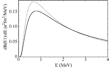
Figure 1: The E1 strength function of ${{}^{8}}\mathrm{B}$. Although the total strengths are the same in these examples, the shapes are very different when treating the ${{}^{8}}\mathrm{B}$ nucleus as a two-body (dotted line) or a three-body (solid line) system. The difference is mainly due to the stronger centrifugal barrier in the three-body case (see, e.g., Ref. Delves (1960)) which forces the WF to be narrower in coordinate space and thus wider in momentum/energy space. The parameters of the model WFs can be found in Table 1.

Table 1: Parameters of our model WFs used to describe the ${{}^{8}}\mathrm{B}$ ground state. Both models give the same intercluster distance, $r_{\mathrm{rms}}=4.57$ fm. With $E_{0}=137$ keV we get $\kappa_{0}=0.076$ fm^-1 and $\eta_{0}=1.595$. The excited core component (last row) has $E_{0}=566$ keV giving $\kappa_{0}=0.154$ fm^-1 and $\eta_{0}=0.786$. The relative orbital momentum for all components are $l_{0}=1$ while $I$ is the channel spin and $a^{2}$ is the spectroscopic factor. Note that there is no dependence on the particular value of the channel spin in the two-body case.

Model WF	configuration	$I$	$a^{2}$	$p$	$\kappa_{1}$ (fm-1)	$\eta_{0}^{\prime}/\eta_{0}$
two-body	$[{{}^{7}}\mathrm{Be}(3/2^{-})\otimes p]$	2	1.00	3	0.601	0.79
	$[{{}^{7}}\mathrm{Be}(3/2^{-})\otimes p]$	2	0.65	5	0.702	0.87
	$[{{}^{7}}\mathrm{Be}(3/2^{-})\otimes p]$	1	0.13	5	0.765	0.86
three-body	$[{{}^{7}}\mathrm{Be}(1/2^{-})\otimes p]$	1	0.16	5	0.753	1.43

However, concerning the structure of the ${{}^{8}}\mathrm{B}$ ground state one should keep in mind that the ${{}^{7}}\mathrm{Be}$ core is in itself a weakly bound system with an excited $1/2^{-}$ state at 429 keV. The common treatment of ${{}^{8}}\mathrm{B}$ as a pure two-body system is therefore questionable. We want to investigate what effect the many-body structure of ${{}^{8}}\mathrm{B}$ might have on the strength function. For this purpose we utilize a recent three-body ($\alpha+{}^{3}\mathrm{He}+p$) calculation Grigorenko et al. (1999) where it was shown that, after projection onto the two-body channels, there are three main components (adding up to 94% of the total WF, see Table 1) and that the rest are pure three-body channels. For each of the numerical two-body overlap functions we fit our parameters $\kappa_{1}$ and $\eta_{0}^{\prime}$. The binding energy, $E_{0}=137$ keV, determines $\kappa_{0}$ for the two first components and $E_{0}=566$ keV for the third, ${{}^{7}}\mathrm{Be}$ excited state, component. The best fit to the small $r$ behavior is obtained with $p=5$ which reflects the effectively larger centrifugal barrier in the three-body case. This centrifugal barrier will push the WF away from $r=0$ and will, thus, force it to become more narrow than the corresponding two-body WF.

III.4 Studies of the corresponding potential

Using the two-body WF (11), which describes correctly the binding energy and the geometry, we are able to restore the corresponding two-body potential. Besides centrifugal barrier and Coulomb interaction, the potential also contains an attractive part which we find can be approximated with a high accuracy by one or two Yukawa-type potentials. Note that such potentials are widely used in few-body nuclear physics. In Fig. 2 the nuclear part of the potential which corresponds to our ${{}^{8}}\mathrm{B}$ “exact” two-body WF is plotted. As is shown in the figure, the potential can be very well described by a Yukawa-type potential. In this connection we would also like to point out that for the special case where $l_{0}=0$ and $Z_{x}=0$, the WF can be described by (20) and the corresponding potential reduces to a Hulthén potential which has exact solutions.

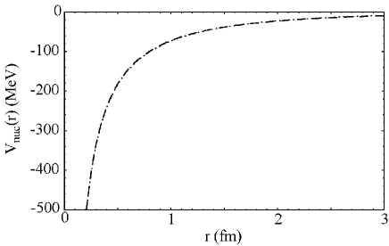
Figure 2: The nuclear potential (dotted line) corresponding to our ${{}^{8}}\mathrm{B}$ “exact” WF. This potential is very well described by a Yukawa potential $V_{\mathrm{nuc}}(r)=-114e^{-0.457r}/r$ (MeV) (dashed line).

IV Electromagnetic dissociation

The EMD of loosely bound nuclei, impinging on a high-$Z$ target, has been used in nuclear physics for many years both in order to investigate nuclear structure and as an indirect method to extract information on radiative capture reactions. Unfortunately, as for all reaction experiments, a lot of information is contained in the experimental results and it is a hard task to disentangle the desired part. The transition matrix elements represents the probability for an initial state wave function to end up in a specific final state after being filtered through the reaction mechanism. Naturally, both the structure of the initial as well as the final state are important for this quantity. In addition, further complications arise if nuclear induced breakup contributes to the measured cross section, and/or if the interaction time is long enough for higher-order transitions to become important. Therefore, in order to minimize interference from higher-order dynamical effects and from nuclear interactions, we will be interested in high-energy experiments in which events characterized by large impact parameters have been selected.

In this section we will demonstrate that the analysis of EMD energy spectra from loosely bound nuclei is highly model dependent. We will then discuss the important issue of how to separate the contributions from specific multipoles; a problem which is of great significance when extracting information on the inverse, radiative capture reaction.

IV.1 Model dependence of energy spectrum analysis

Applying our analytical model to study EMD using first-order perturbation theory enables us to investigate the sensitivity of the energy spectrum to some properties of the initial bound state. At small relative energies the electromagnetic processes are highly peripheral, which means that the interaction mainly probes the external part of the bound state WF. As a consequence, the amplitude of the EMD cross section should depend crucially on the size of the nuclear system. A larger size implies a lower Coulomb barrier, which results in a larger tunneling probability, and consequently a larger cross section. However, the radii of nuclei far from stability are usually extracted from interaction cross section measurements, and this procedure has unfortunately proven to be highly model dependent. A Glauber-type analysis, assuming a uniform density distribution, results in a smaller radius as compared to an analysis in which the few-body structure is taken into account explicitly Al-Khalili and Tostevin (1996). Furthermore, the relevant parameter for two-body breakup is in reality the intercluster distance rather than the total matter radius, and the relation between these two quantities is also model dependent. In a pure two-body model one often assumes that the size of the core is equal to the size of the corresponding free nucleus. In contrast, taking many-body structure into account will result in polarization effects. For example, it was found in Ref. Grigorenko et al. (1998) that the average distance between ${{}^{3}}\mathrm{He}-\alpha$ is approximately 10% smaller inside ${{}^{8}}\mathrm{B}$ (studied in a ${{}^{3}}\mathrm{He}+\alpha+p$ picture) than in a free ${{}^{7}}\mathrm{Be}$ nucleus (${{}^{3}}\mathrm{He}+\alpha$ picture).

We have investigated the sensitivity of the EMD cross section to the rms intercluster distance by performing model calculations with a ${{}^{8}}\mathrm{B}$-like system. A pure two-body system with $l_{0}=1$ relative motion (having unity spectroscopic factor) was assumed and a binding energy of 0.137 MeV was used. The effective Sommerfeld parameter was fitted to the asymptotic behavior of (11), i.e., to the Whittaker tail. The size of our model WF (13) was then a function of the remaining free parameter $\kappa_{1}$. By varying this parameter we could investigate the sensitivity to the size and from Fig. 3 it is clear how strong it is. Just for illustration: a 15% uncertainty in the rms intercluster distance (which, in our model, would correspond to 5% uncertainty in the ${{}^{8}}\mathrm{B}$ matter radius) results in $\sim 50$% ambiguity of the calculated total cross section.

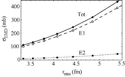
Figure 3: The total EMD cross section as a function of intercluster distance. The parameter $\kappa_{1}$ of our two-body model WF was varied in order to change the rms distance between the ${{}^{7}}\mathrm{Be}$ core and the valence proton. A beam energy of 82.7 MeV/nucleon and a minimum impact parameter of 30 fm was used.

Let us now consider the difference between a two-body and a three-body approach. As was mentioned in Sec. III.3, the effectively larger centrifugal barrier in a three-body system will push the relative motion WF away from $r=0$ and consequently force it to become more narrow than the corresponding two-body WF for a given radius. We therefore expect the distribution in momentum/energy space to be broader. This effect is clearly seen in Fig. 1 where the ${{}^{8}}\mathrm{B}$ E1 strength functions, obtained using our three-body  and two-body analytical model WFs, are compared. This difference, seen in the strength function, should be even more pronounced in the energy spectrum since it will be magnified by the spectrum of virtual photons.

In Fig. 4 we compare different calculations of ${{}^{8}}\mathrm{B}$ EMD on Pb, including both E1 and E2 transitions, to the experimental data from Davids et al. Davids et al. (2001). This experiment is very appealing since the selection of scattering angles ($\theta_{{{}^{8}}\mathrm{B}}\leq 1.77^{\circ}$, which corresponds to a minimum impact parameter of $b_{\mathrm{min}}=30$ fm) minimizes the contribution from nuclear scattering, and the relatively high beam energy (82.7 MeV/nucleon) justifies the use of first-order perturbation theory. Let us first compare our analytical two-body (dotted line) and three-body (solid line) results, see also Ref. Forssén et al. (2002a). Concerning the shape of the energy spectrum we have an excellent agreement between the experimental data and our results obtained using the three-body model, while the pure two-body calculation gives a too narrow peak. As to the absolute values, the three-body energy spectrum is approximately 20% above the experimental data. However, the most important lesson from this comparison is that for two different assumptions concerning the nuclear structure, but keeping the rms intercluster distance fixed, we obtain very different shapes of the calculated energy spectra. Thus, one can conclude that the interpretation of energy spectra is highly model dependent. A final remark in connection to this observation is that, in order to interpret experimental data correctly, it is very important to fix the spectroscopic factors of different two-body and many-body components. Therefore, we want to stress the usefulness of experiments where EMD is studied in complete kinematics. Examples of interesting channels in the ${{}^{8}}\mathrm{B}$ case is ${{}^{8}}\mathrm{B}\rightarrow{{}^{7}}\mathrm{Be}(1/2^{-})+p+\gamma$ and ${{}^{8}}\mathrm{B}\rightarrow{{}^{3}}\mathrm{He}+\alpha+p$. Some progress has already been made in this direction. Recently, ${{}^{7}}\mathrm{Be}$ fragments and $\gamma$-rays were measured in coincidence after breakup on a light target by Cortina-Gil et al. Cortina-Gil et al. (2002) which resulted in a clear observation of the excited core component of the WF.

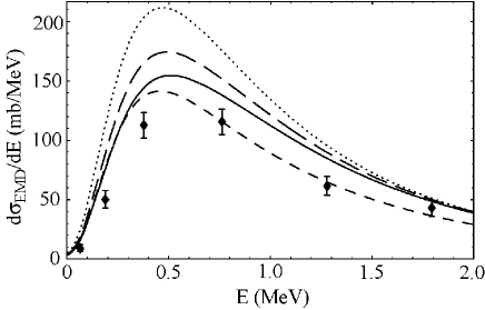
Figure 4: The ${{}^{8}}\mathrm{B}$ EMD energy spectrum obtained at 82.7 MeV/nucleon on Pb with ${{}^{8}}\mathrm{B}$ scattering angles $\theta_{{{}^{8}}\mathrm{B}}\leq 1.77^{\circ}$. The data points are from Davids et al. (2001). The curves show our analytical two-body (dotted line) and three-body (solid line) results, and the numerical calculations: without FSI (long-dashed), and with FSI (short-dashed). All theoretical curves have been corrected for experimental resolution and acceptance.

We have also performed numerical calculations, based on first-order perturbation theory, where the numerical ${{}^{8}}\mathrm{B}$ bound state WF from Grigorenko et al. (1999) was used. In the first investigation we assumed a pure Coulomb continuum and the results of this calculation is shown as a long-dashed line in Fig. 4. We note that the obtained energy spectrum compares rather well with our analytical three-body model except for a 15% difference in the peak height. Since our analytical model has the correct asymptotic behavior for large $r$ and a three-body behavior at small $r$, the main difference to the numerical WF should be in the intermediate region, and this is exactly the region which dominates the transition matrix elements for energies corresponding to the peak of the energy spectrum. This fact explains the observed discrepancy.

In our second numerical investigation we studied the influence of ${{}^{7}}\mathrm{Be}+p$ FSI. As previously mentioned, the low-energy continuum of ${{}^{8}}\mathrm{B}$ is dominated by positive parity states Ajzenberg-Selove (1988) which are only relevant for E2 ($\sim$10% of the total cross section) and M1 transitions. Note that the latter only plays a role in the vicinity of the narrow $1^{+}$ resonance at 0.64 MeV above threshold, and is therefore not included in our calculations. However, the possible existence of a very broad negative parity state at high excitation energy can still have a strong influence on the energy spectrum. Effects of such a state was observed in a recent elastic proton scattering experiment Rogachev et al. (2001) from which the authors made a $2^{-}$ spin-parity assignment and, from an $R$-matrix analysis, they obtained a best fit with the parameters $E=3.5\pm 0.5$ MeV and $\Gamma=8\pm 4$ MeV. We have included such a broad continuum structure by adding an attractive potential in the $s$-wave channel. The effects of this are clearly seen in Fig. 4 (short-dashed line): the total cross section is reduced and the continuum strength is redistributed towards smaller energies. We conclude this comparison by stating that a broad negative parity structure in the high energy continuum has a non-negligible influence on the EMD energy spectrum for energies $\gtrsim 0.4$ MeV and that the parameters of such a state are still to be determined with greater accuracy.

IV.2 Extraction of E1 contribution using the low-$\bm{E}$ energy spectrum

As we have seen in the previous section the main model uncertainties in the EMD analysis are: the asymptotic normalization constant which depends on (i) the radius in combination with (ii) the spectroscopic factors of different two-body components; (iii) the underlying many-body structure, and finally; (iv) the FSI. Despite the difficulties connected with measuring the cross section at small relative energies, we still suggest to focus on the low-$E$ part of the energy spectrum. In this way one can avoid uncertainties associated with FSI (unless there are resonances very close to threshold) and with the many-body behavior of the WF at small intercluster distances. The asymptotic normalization constant in combination with the spectroscopic factor will enter as an absolute normalization of the cross section. However, since this normalization affects all multipole transitions equally it is possible to calculate the ratio of two different multipoles with a very good precision.

We have investigated the ratio

$$R_{\mathrm{EMD}}(E)\equiv\frac{\mathrm{d}\sigma_{\mathrm{EMD}}(\mathrm{E}1)/\mathrm{d}E}{\mathrm{d}\sigma_{\mathrm{EMD}}(\mathrm{E}1+\mathrm{E}2)/\mathrm{d}E},$$ (23)

and found that it is almost model independent at small relative energies. To demonstrate this we will continue to use the EMD of ${{}^{8}}\mathrm{B}$ (on a Pb target at 82.7 MeV/nucleon with $b_{\mathrm{min}}=30$ fm) as an example. Reusing the different model calculations from Sec. IV.1 we can investigate the sensitivity of the ratio to different model assumptions. Firstly, in Fig. 5 we can see that the difference between a two-body and a three-body approach is less than 3% in the region of interest. This low sensitivity can be explained by the fact that the low-$E$ part of the spectrum mainly probes the large $r$ asymptotics of the radial WF. Shown in Fig. 5 are also results from the numerical calculations introduced in Sec. IV.1. It is clearly seen that the influence from FSI is almost negligible at small relative energies where the numerical results and our analytical three-body model seem to converge. Unfortunately, the numerical accuracy of our calculations becomes questionable at small energies and the calculated ratio is therefore only plotted down to 0.1 MeV. In this context we want to stress that in our analytical model we are able to calculate the relevant transition matrix elements for all energies, including the limit $E\to 0$. In contrast, the numerical approaches will run into problems for small energies since the continuum WF will be extremely small at relevant intercluster distances.

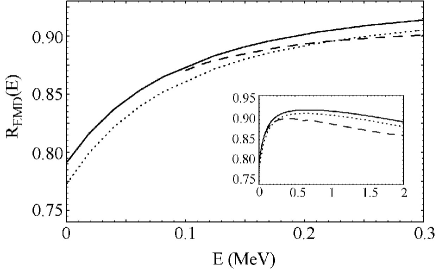
Figure 5: Fraction of the calculated energy spectrum (EMD of 82.7 MeV/nucleon ${{}^{8}}\mathrm{B}$ on Pb with scattering angles $\theta_{{}^{8}}\mathrm{B}\leq 1.77^{\circ}$) attributed to E1 transitions, see Eq. (23). The curves show two-body (dotted line) and three-body (solid line) analytical results while the dashed line shows results of numerical calculations including FSI. The inset shows the same curves for a broader energy range.

Furthermore, as can be seen in Fig. 6, the sensitivity of the $R_{\mathrm{EMD}}(E)$ ratio (23) to the intercluster distance is also very small. This feature is also expected since the intercluster distance determines the asymptotic normalization of the WF which, in turn, cancels when the ratio is calculated. However, as can be seen in the insets of Figs. 5 and 6, the results obtained using the different models diverge with increasing energy.

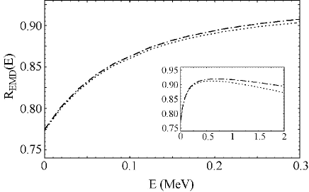
Figure 6: Fraction of the calculated energy spectrum (EMD of 82.7 MeV/nucleon ${{}^{8}}\mathrm{B}$ on Pb with scattering angles $\theta_{{}^{8}}\mathrm{B}\leq 1.77^{\circ}$) attributed to E1 transitions, see Eq. (23). The curves show two-body results characterized by two different intercluster distances: $r_{\mathrm{rms}}=3.3$ fm (dash-dotted) and $r_{\mathrm{rms}}=5.4$ fm (dotted). The inset shows the same curves for a broader energy range.

One final question is well-founded: Since the transition matrix elements for very small energies depend mainly on the tail of the bound state WF, is it still justified to use our model WF (13) which has merely an approximate description of the Whittaker tail? The result of our numerical calculation (remember that the numerical bound state WF has the correct asymptotics) presented in Fig. 5 indicates that it is justified, since it seems to converge with the analytical model for small $E$. Furthermore, in the limit $E\to 0$ we are actually able to solve the radial integral (10) exactly even for the “exact” WF (11) which has a Whittaker tail. We find that $R_{\mathrm{EMD}}(E\to 0)$ calculated with the model WF and with the “exact” WF agree within 0.5%. This result gives an additional justification to the use of our model WF for calculating transition matrix elements at small $E$.

In summary we have found that the calculated $R_{\mathrm{EMD}}(E)$ ratio of the energy spectrum is almost model independent at small relative energies. In first-order perturbation theory this ratio can be expressed as

$$R_{\mathrm{EMD}}(E) \equiv\frac{\mathrm{d}\sigma_{\mathrm{EMD}}(\mathrm{E}1)/\mathrm{d}E}{\mathrm{d}\sigma_{\mathrm{EMD}}(\mathrm{E}1+\mathrm{E}2)/\mathrm{d}E}$$ (24)

$$=1\Big{/}\left(1+\frac{n_{\mathrm{E}2}(E_{\gamma})}{n_{\mathrm{E}1}(E_{\gamma})}\frac{\sigma_{\gamma}^{\mathrm{E}2}(E)}{\sigma_{\gamma}^{\mathrm{E}1}(E)}\right)$$

$$=1\Big{/}\left(1+\frac{n_{\mathrm{E}2}(E_{\gamma})}{n_{\mathrm{E}1}(E_{\gamma})}r_{\gamma}(E)\right),$$

where we have introduced the E2/E1 ratio of photo-dissociation cross sections

$$r_{\gamma}(E)\equiv\frac{\sigma_{\gamma}^{\mathrm{E}2}(E)}{\sigma_{\gamma}^{\mathrm{E}1}(E)}.$$ (25)

Naturally, the ratio $R_{\mathrm{EMD}}(E)$ will depend on the experimental conditions such as beam energy and minimum impact parameter. However, this dependence enters only in the spectra of virtual photons which are easily calculated for any experimental conditions $\left\{b_{\mathrm{min}},E_{\mathrm{beam}}\right\}$ (see, e.g., Eq. (4.7) of Bertulani and Baur (1985)). In contrast, the ratio of ${{}^{8}}\mathrm{B}$ photo-dissociation cross sections $r_{\gamma}(E)$ (25) does not depend on the experimental conditions. Therefore, we provide this ratio, calculated within our analytical three-body model, in Fig. 7. The curve shown in Fig. 7 can approximately be described by the formula

$$r_{\gamma}(E)=\frac{\sigma_{\gamma}^{\mathrm{E}2}(E)}{\sigma_{\gamma}^{\mathrm{E}1}(E)}=\left(-1.7290+3.4663e^{1.5526E}\right)\cdot 10^{-4},$$ (26)

which describes the calculated curve with an accuracy of $<0.5$% in the region $0<E<0.3$ MeV. From this formula it is easy to obtain $R_{\mathrm{EMD}}(E)$ using Eq. (24)

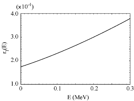
Figure 7: Ratio of photo-dissociation cross sections calculated within our analytical three-body model, see Eq. (25).

IV.3 Extraction of E1 contribution using two different experimental conditions

One of the beauties with the method of virtual photons is the separation of reaction kinematics and nuclear excitation dynamics into the spectrum of virtual photons and the photo-absorption cross section, respectively. This separation can be used as an alternative method to extract the E1 contribution from the measured cross section. The objective is to use the fact that the cross section will depend on beam energy and minimum impact parameter only through the spectra of virtual photons. First, let us introduce the notation

$$N_{\mathrm{E}\lambda}(E_{\gamma})=\frac{n_{\mathrm{E}\lambda}(E_{\gamma},b_{\mathrm{min}},E_{\mathrm{beam}})}{E_{\gamma}},$$ (27)

where we have indicated that the spectra of virtual photons are functions of the beam energy and minimum impact parameter. In reality this dependence enters in the adiabaticity parameter

$$\xi=\frac{\omega b_{\mathrm{min}}}{\gamma v}.$$ (28)

Assuming that the total cross section is dominated by E1 and E2 transitions we find that the energy spectrum for given experimental conditions $\{b_{\mathrm{min}}^{(i)},E_{\mathrm{beam}}^{(i)}\}$ is given by

$$\frac{\mathrm{d}\sigma_{\mathrm{EMD}}^{(i)}}{\mathrm{d}E}=N_{\mathrm{E}1}^{(i)}(E_{\gamma})\sigma_{\gamma}^{\mathrm{E}1}(E)+N_{\mathrm{E}2}^{(i)}(E_{\gamma})\sigma_{\gamma}^{\mathrm{E}2}(E),$$ (29)

where we would like to remind the reader of the relation $E=E_{\gamma}-E_{0}$. Now we can use the fact that the virtual photon spectra depends differently on $\xi$ for different multipoles to extract the contribution from one of the multipoles. Let us assume that we have two sets of experimental data from the same experimental setup; the only difference being the beam energy and/or the selected scattering angles (minimum impact parameter). The E1 contribution to one of the measurements can then be obtained with the formula

$$\frac{\mathrm{d}\sigma_{\mathrm{EMD}}^{(1)}(\mathrm{E}1)}{\mathrm{d}E}=\left(N_{\mathrm{E}2}^{(2)}(E_{\gamma})\frac{\mathrm{d}\sigma_{\mathrm{EMD}}^{(1)}}{\mathrm{d}E}-N_{\mathrm{E}2}^{(1)}(E_{\gamma})\frac{\mathrm{d}\sigma_{\mathrm{EMD}}^{(2)}}{\mathrm{d}E}\right)\\ \times\frac{N_{\mathrm{E}1}^{(1)}(E_{\gamma})}{N_{\mathrm{E}1}^{(1)}(E_{\gamma})N_{\mathrm{E}2}^{(2)}(E_{\gamma})-N_{\mathrm{E}1}^{(2)}(E_{\gamma})N_{\mathrm{E}2}^{(1)}(E_{\gamma})}.$$ (30)

The advantage of this method is that information can be obtained directly from experimental data. However, it should be emphasized that the formula is only valid under the assumptions of first-order perturbation theory and straight-line trajectories. Thus, this method can only be used for EMD at relatively large beam energies where events characterized by large impact parameters have to be selected. Furthermore, the experimental conditions must be chosen so that the difference $\mathrm{d}\sigma_{\mathrm{EMD}}^{(1)}/\mathrm{d}E-\mathrm{d}\sigma_{\mathrm{EMD}}^{(2)}/\mathrm{d}E$ is observable and larger than the experimental uncertainty.

V Conclusion

In this paper we have studied electromagnetic processes involving loosely bound nuclei. To this aim we have developed an analytical model which is based on the use of radial model functions that give a realistic description of two-body WFs (or the two-body projections of many-body WFs) for all radii, see also Forssén et al. (2002a). We have used this model to study EMD of ${{}^{8}}\mathrm{B}$, but have also indicated how it can be applied to other reactions and other nuclei. For example, it should provide an important tool to investigate the low-energy behavior of the astrophysical $S$-factor.

We have also presented numerical calculations based on the three-body model of ${{}^{8}}\mathrm{B}$, developed in Ref. Grigorenko et al. (1999), and on recent experimental information on a broad negative parity state in the ${{}^{8}}\mathrm{B}$ continuum. Combining the results of our analytical model, and of these numerical calculations, has allowed us to investigate the sensitivity of calculated EMD energy spectra to different model assumptions. We concluded that the magnitude of the cross section depends strongly on the intercluster distance and on the spectroscopic factors of different many-body channels; while the shape of the energy spectrum is very sensitive to the few-body structure. Finally, we found that a broad negative parity state at high excitation energy will influence the energy spectrum for energies $\gtrsim 0.4$ MeV, and will lead to a reduction of the cross section.

However, the main purpose of this paper has been to investigate the problem of how to extract the E1 contribution from a measured EMD energy spectrum. This question is of great significance for the gathering of information on astrophysically interesting radiative capture reactions from EMD experiments (note the relation between the E1 component of the EMD energy spectrum and the astrophysical $S$-factor via Eqs. (4–6)). The main method so far has been to study the asymmetries in angular or momentum distributions. However, this asymmetry (which is due to E1-E2 interference) depends strongly on details of the FSI which, in turn, are often relatively unknown. Furthermore, the E1-E2 interference terms do not themselves contribute to the integrated cross sections to which the $S$-factor is related. Instead, we have proposed two novel, and less model dependent, approaches to extract the E1 contribution from a measured EMD energy spectrum: (i) Firstly, we demonstrated that the ratio of EMD cross sections $\sigma_{\mathrm{EMD}}(\mathrm{E}1)/\sigma_{\mathrm{EMD}}(\mathrm{E}1+\mathrm{E}2)$ is almost model independent at small relative energies. We also provided an analytical formula to calculate this ratio for any experimental conditions. (ii) Secondly, we demonstrated how two sets of experimental data, obtained with different $E_{\mathrm{beam}}$ and/or $b_{\mathrm{min}}$, can be used to extract the E1 component. This method relies on the fact that the strengths of different multipole components depend on the beam energy and minimum impact parameter, and in first-order perturbation theory this dependence enters only in the virtual photon spectra.

Since the proposed two methods are not directly connected to each other, they can be used independently and the results can be compared to each other. However, both methods, but in particular the first one, require that the energy spectrum is measured down to very small relative energies (100–300 keV), which will probably prove to be a difficult challenge.