New treatment of breakup continuum
in the method of continuum discretized coupled channels

Abstract

A new method of pseudo-state discretization is proposed for the method of continuum discretized coupled channels (CDCC) to deal with three-body breakup processes. We propose real- and complex-range Gaussian bases for the pseudo-state wave functions, and show that they form in good approximation a complete set in the configuration space which is important for breakup processes. Continuous S-matrix elements are derived with the approximate completeness from discrete ones calculated by CDCC. Accuracy of the method is tested quantitatively for two realistic examples, $d$+⁵⁸Ni scattering at 80 MeV and ⁶Li+⁴⁰Ca scattering at 156 MeV with the satisfactory results. Possibility of application of the method to four-body breakup processes is also discussed.

I Introduction

The method of continuum discretized coupled channels (CDCC) has been successful in describing nuclear reactions including weakly bound projectiles CDCC-review1 ; CDCC-review2 ; Yahiro1 ; yahiro2 ; sakuragi1 ; sakuragi2 ; sakuragi3 ; sakuragi4 ; iseri1 ; Sakuragi ; Surrey ; Ogata . CDCC has been attracting much attention since the advent of experiments with radioactive beams, because projectile breakup processes are essential to many of such reactions. CDCC plays an important role in the spectroscopic studies of radioactive nuclei through the nuclear reactions involving such nuclei.

In CDCC for reactions with a projectile consisting of two fragments, the states of the projectile are classified by the linear and the angular momenta, $k$ and $\ell$, of relative motion of the two fragments of the projectile, which are truncated by $k\leq k_{\rm max}$ and $\ell\leq\ell_{\rm max}$. The truncation is the most basic assumption in CDCC, and it is confirmed that calculated $S$-matrix elements converge for sufficiently large $k_{\rm max}$ and $\ell_{\rm max}$ CDCC-review1 ; Yahiro1 ; Piya . It has been shown that CDCC is the first-order approximation to the distorted Faddeev equations, and corrections to the converged CDCC solution are negligible within the region of space in which the reaction takes place CDCC-foundation .

As a consequence of the truncation, the integral equation form of the equations of coupled channels, derived from the three-body Schrödinger equation, has a compact kernel, satisfying a necessary condition for iterative solutions CDCC-foundation . In practice, however, the coupled channels equations thus obtained are impossible to be solved because of the continuously infinite number of coupled breakup channels. The problem is solved by discretizing the $k$ continuum. The discretization leads the coupled equations to a set of differential equations with a finite number of channels.

As for the discretization, three methods have been proposed so far: the average (Av) YK1 ; Yahiro1 ; CDCC-review1 ; CDCC-review2 , the midpoint (Mid) CDCC-review2 ; Piya , and the pseudo-state (PS) CDCC-review1 ; PS1 ; PS2 methods. In the Av and Mid methods, the $k$-continuum is divided into a finite number of bins. In the former the continuum channels within each bin are averaged into a single channel, while in the latter they are represented by the channel at a midpoint of the bin. It has been confirmed that calculated $S$-matrix elements converge as the width $\Delta$ of the bins is decreased, and also that the two methods yield the same converged $S$-matrix elements CDCC-review1 ; Yahiro1 ; Piya . From practical point of view, the Av method is more convenient than the Mid one, since the former requires less numerical works than the latter. The Av method therefore is most widely used in practice.

In the PS method, the breakup states are described by superpositions of $L^{2}$-type basis functions. The wave functions of such pseudo breakup state have wrong asymptotic forms. For this reason, the PS method was mainly used in the past to describe virtual breakup processes in the intermediate stage of elastic scattering and ($d,p$) reactions. Very recently, the applicability of the PS method for real breakup reactions for a specific set of basis functions. It was shown that the PS method well simulates the angular distribution of the total breakup cross section calculated with the Av method  PS1 . In the analysis, discrete breakup cross sections calculated with the PS method are transformed into continuous one, by assuming a specific form for the $k$ distribution of the continuous cross section, that is, a histogram with widths estimated in a reasonable way.

The purpose of the present paper is to propose a new PS method for projectile breakup reactions. If the basis functions form in the good approximation a complete set in the configuration space which is important for breakup processes, we can formulate a method of interpolation for generating continuous breakup $S$-matrix elements from the discrete ones provided by the PS method, following the formulation of Tostevin for the Av method in which the completeness of discretized states is well satisfied if the discretization is enough precise. The method does not assume any form a priori for $k$ distributions of continuous breakup $S$-matrix elements. The method is independent of the type of the basis functions used for the PS method. Only condition is that the basis functions constitute an approximate complete set in the wide range of $k$ and its conjugate coordinate $r$ which are important for the breakup processes. As basis functions satisfying this condition, we propose two types of them. One is ordinary Gaussian functions K-G , which we refer to as real-range Gaussian function in the present paper. The other is a natural extension of that, complex-range Gaussian function H-Ka-Ki , i.e, Gaussian functions with the complex range parameters the precise definition of which is given in a later section.

In Section II, we recapitulate CDCC based on both the Av and the PS methods of discretization. In Section III, we present a method of interpolation to get continuous breakup $S$-matrix elements from discrete ones calculated with the PS method, and introduce the real and the complex-range Gaussian basis. In Section IV, the validity of the present PS method is tested and justified for two realistic cases, $d$+⁵⁸Ni scattering at 80 MeV and ⁶Li+⁴⁰Ca scattering at 156 MeV. In Section V, the potentiality of the present PS method for four-body breakup reactions is discussed. Section VI gives a summary.

II The Method of Continuum Discretized Coupled Channels

We consider a reaction of a weakly bound projectile (B) impinging on a target nucleus (A). We treat a simple system shown in Fig. 1 in which the projectile, B, is composed of two particles (b and c) and the target is inert. The three-body system is described by a model Hamiltonian $H=H_{\rm bc}+K_{R}+U,$ where $H_{\rm bc}=K_{r}+V_{\rm bc}({\bf r})$ and $U=U_{\rm bA}({\bf r}_{\rm bA})+U_{\rm cA}({\bf r}_{\rm cA})$. Vector ${\bf r}$ is the relative coordinate between b and c, ${\bf R}$ the one between the center-of-mass of the b-c pair and the center-of-mass of A, and ${\bf r}_{\mathrm{XY}}$ denotes the relative coordinate between two particles X and Y. Operators $K_{r}$ and $K_{R}$ are kinetic energies associated with ${\bf r}$ and ${\bf R}$, respectively. $V_{\rm bc}({\bf r})$ is the interaction between b and c. The interaction $U_{\rm bA}$ ($U_{\rm cA}$) between b (c) and A is taken to be the optical potential for b+A (c+A) scattering. For simplicity, the spin dependence of the interactions is neglected. Furthermore, the Coulomb part of $U$ is treated approximately as a function only of ${\bf R}$, i.e., we neglect Coulomb breakup processes, and focus our attention on nuclear breakup.

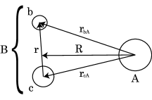
Figure 1: Illustration of a three-body (A+b+c) system. The symbol B=b+c stands for the projectile, and A is the target.

In CDCC, the three-body wave function $\Psi_{JM}$, with the total angular momentum $J$ and its projection $M$ on $z$-axis, is expanded in terms of the orthonormal set of eigenstates $\Phi$ of $H_{\rm bc}$:

$$\Psi_{JM}({\bf r,R})=\sum_{L}{\cal Y}_{JM}^{\ell_{0},L}\Phi_{0}(r)\chi_{\ell_{0}LJ}(P_{0},R)/R$$

$$+\sum_{\ell,L}{\cal Y}_{JM}^{\ell,L}\int_{0}^{\infty}\Phi_{\ell}(k,r)\chi_{\ell LJ}(P,R)/R\,\;dk,$$ (1)

where

$${\cal Y}_{JM}^{\ell,L}=[i^{\ell}Y_{\ell}(\Omega_{r})\otimes i^{L}Y_{L}(\Omega_{R})]_{JM}.$$ (2)

For simplicity, we assume that the b+c system has one bound state $\Phi_{0}(r)$ with angular momentum $\ell_{0}$ and continuum states $\Phi_{\ell}(k,r)$ with linear momentum $k$ and angular momentum $\ell$, both ranging from zero to infinity. The $\Phi_{\ell}$ are real functions normalized to the $\delta$-function in $k$ Yahiro1 . The projectile B is initially in the bound state. The coefficient $\chi_{\ell LJ}$ ($\chi_{\ell_{0}LJ}$) of the expansion describes a center-of-mass motion of the b-c pair relative to A in the state $\Phi_{\ell}$ with the linear and orbital angular momenta $P$ $(P_{0})$ and $L$, respectively.

In CDCC, the sum over $\ell$ is truncated by $\ell\leq\ell_{\rm max}$ and the $k$ integral by $k\leq k_{\rm max}$. For each $\ell$, furthermore, the continuum states from $k=0$ to $k_{\rm max}$ are discretized into a finite number of states, with the wave function $\hat{\Phi}_{i\ell}(r)$ of the i-th state corresponding to the momentum $\hat{k}_{i}$. Details of the discretization methods are described in the next section.

After the truncation and the discretization, $\Psi_{JM}$ is reduced to an approximate one,

$$\Psi^{\rm CDCC}_{JM}=\sum_{L}{\cal Y}_{JM}^{\ell_{0},L}\Phi_{0}(r)\hat{\chi}_{\gamma_{0}}(P_{0},R)/R$$

$$+\sum_{l=0}^{l_{\rm max}}\sum_{i=1}^{N}\sum_{L}{\cal Y}_{JM}^{\ell,L}\hat{\Phi}_{i\ell}(r)\hat{\chi}_{\gamma}(\hat{P}_{i},R)/R,$$ (3)

where

$$\hat{\chi}_{\gamma_{0}}(P_{0},R) = \chi_{\gamma_{0}}(P_{0},R),\;\;\;\gamma_{0}=(0,\ell_{0},L,J),$$

$$\hat{\chi}_{\gamma}(\hat{P}_{i},R) = W_{\gamma}\chi_{\gamma}(\hat{P}_{i},R),\;\;\;\gamma=(i,\ell,L,J).$$

On the right hand side of Eq. (3), the first term represents the elastic channel denoted by $\gamma_{0}$ and the second one corresponds to the discretized breakup channels, each denoted by $\gamma$. The weight factor $W_{\gamma}$ depends on the discretization method used. Each pair of momenta, $(\hat{k}_{i},\hat{P}_{i})$, satisfies the total energy conservation:

$$E=\hbar^{2}P_{0}^{2}/2\mu_{\rm AB}+\epsilon_{0}=\hbar^{2}\hat{P}_{i}^{2}/2\mu_{\rm AB}+\epsilon_{i},$$ (4)

where $\epsilon_{0}$ and $\epsilon_{i}=\hbar^{2}\hat{k}_{i}^{2}/2\mu_{\rm bc}$ are the energies of the ground and the continuum states, respectively. Inserting Eq. (3) into the three-body Schrödinger equation, $(H-E)\Psi_{JM}=0$, leads to a set of coupled differential equations for $\hat{\chi}_{\gamma_{0}}(P_{0},R)$ and $\hat{\chi}_{\gamma}(\hat{P}_{i},R)$:

$$\left[\frac{d^{2}}{dR^{2}}+\hat{P}_{i}^{2}-\frac{L(L+1)}{R^{2}}-\frac{2\mu_{\rm AB}}{\hbar^{2}}V_{\gamma\gamma}(R)\right]\hat{\chi}_{\gamma}(\hat{P}_{i},R)$$

$$=\sum_{\gamma^{{}^{\prime}}\neq\gamma}\frac{2\mu_{\rm AB}}{\hbar^{2}}V_{\gamma\gamma^{{}^{\prime}}}(R)\hat{\chi}_{\gamma^{{}^{\prime}}}(\hat{P}_{i^{{}^{\prime}}},R)$$ (5)

for all $\gamma$ including $\gamma_{0}$, where $\hat{k}_{0}=\sqrt{-2\mu_{\rm bc}\epsilon_{0}}/\hbar$ and $\hat{P}_{0}=P_{0}$. The coupling potentials $V_{\gamma\gamma^{{}^{\prime}}}(R)$ are obtained as

$$V_{\gamma\gamma^{{}^{\prime}}}(R)=\langle{\cal Y}_{JM}^{\ell,L}\hat{\Phi}_{i\ell}(r)|U|{\cal Y}_{JM}^{\ell^{{}^{\prime}},L^{{}^{\prime}}}\hat{\Phi}_{i^{{}^{\prime}}\ell^{{}^{\prime}}}(r)\rangle_{{\bf r},\Omega_{R}}.$$ (6)

The coupled equations are solved, under the asymptotic boundary condition

$$\hat{\chi}_{\gamma}(\hat{P}_{i},R)\sim u_{L}^{(-)}(\hat{P}_{i},R)\delta_{\gamma,\gamma_{0}}-\sqrt{\frac{\hat{P}_{i}}{\hat{P}_{0}}}\hat{S}_{\gamma,\gamma_{0}}u_{L}^{(+)}(\hat{P}_{i},R).$$ (7)

Here $u_{L}^{(-)}(\hat{P}_{i},R)$ and $u_{L}^{(+)}(\hat{P}_{i},R)$ are incoming and outgoing Coulomb wave functions with the momentum $\hat{P}_{i}$, and $\hat{S}_{\gamma,\gamma_{0}}$ is the $S$-matrix element for the transition from the initial channel $\gamma_{0}$ to $\gamma$.

III Discretization of $k$ continuum

Among the three methods of discretization of the $k$ continuum, the relation between the average (Av) and the midpoint (Mid) methods has already been clarified Piya . The present discussion therefore is focused on the relation between the Av and the pseudo-state (PS) methods.

III.1 The average method

In the Av method, the $k$-continuum [0, $k_{\rm max}$], for each $\ell$, is divided into a finite number of bins, each with a width $\Delta_{i\ell}=k_{i}-k_{i-1}$, and the continuum breakup states in the $i$-th bin are averaged with a weight function $f_{i\ell}(k)$ CDCC-review1 ; CDCC-review2 . The resultant orthonormal state is described as

$$\hat{\Phi}_{i\ell}(r)=\frac{1}{W_{\gamma}}\int_{k_{i-1}}^{k_{i}}\Phi_{\ell}(k,r)f_{i\ell}(k)dk\quad{\mbox{(for Av) ,}}$$ (8)

then the weight factor $W_{\gamma}$ is given by

$$W_{\gamma}^{2}=\int_{k_{i-1}}^{k_{i}}[f_{i\ell}(k)]^{2}\,dk.$$

For a bin far from a resonance, it is natural to set $f_{i\ell}(k)=1$, so that $W_{\gamma}=\sqrt{\Delta_{i\ell}}$ since $\Phi_{\ell}(k,r)$ changes smoothly with $k$. On the other hand, $\Phi_{\ell}(k,r)$ changes rapidly across the resonance. One way of coping with this situation is to take $\Delta_{i\ell}$ much smaller than the width of the resonance so that $\Phi_{\ell}(k,r)$ does not change much within individual bins. This, however, make the number of bins large. Alternatively, one can take a single bin which contains the whole resonance peak and use a weight function of Breit-Wigner type CDCC-review1 ; sakuragi1 ; sakuragi2 ; sakuragi4 ; Sakuragi ,

$$f_{i\ell}(k)=\left|\frac{i\Gamma/2}{\epsilon(k)-\epsilon_{\rm res}+i\Gamma/2}\right|,$$ (9)

where $\epsilon(k)$ is a continuous intrinsic energy of the b+c system. The discretized intrinsic energy, $\epsilon_{i}=\hbar^{2}\hat{k}_{i}^{2}/2\mu_{\rm bc}$, corresponding to each bin is obtained as $\hat{k}_{i}^{2}=(k_{i}+k_{i-1})^{2}/4+\Delta_{i\ell}^{2}/12$ for a non-resonance bin and $\epsilon_{i}=\epsilon_{\rm res}$ for a resonance one. Comparing the approximate form (3) with the exact one (1) in the asymptotic region $R\to\infty$, it is natural to assume

$$S^{(J)}_{\ell,L}(k)\approx\frac{\hat{S}_{\gamma,\gamma_{0}}}{W_{\gamma}}f_{i\ell}(k)\quad{\mbox{(for Av) ,}}$$ (10)

for $k$ belonging to the $i$-th bin, i.e., $k_{i-1}<k\leq k_{i}$.

III.2 The pseudo-state method

In the PS method, $H_{\rm bc}$ is diagonalized in a space spanned by a finite number of $L^{2}$ type basis functions. The resultant eigenstates can well reproduce both bound and continuous states within a finite region of $k$ and $r$ YK1 . The $k$ continuum is automatically discretized by identifying the eigenstates of positive energies with $\hat{\Phi}_{i\ell}(r)$. The weight factor $W_{\gamma}$ is unity if the resultant discretized states $\hat{\Phi}_{i\ell}(r)$ are orthonormalized. Among the eigenstates, only low-lying states belonging to the region $0<\epsilon<\hbar^{2}k_{\rm max}^{2}/2\mu_{\rm bc}$ are taken as breakup channels in CDCC equation (5), where $k_{\rm max}$ is the maximum $k$ in the Av method.

The CDCC equations (5) thus obtained yield discrete breakup $S$-matrix elements. If the basis functions form a complete set with good accuracy in the region of $r$ and $k$ which is important for breakup processes, an accurate transformation from the approximate breakup $S$-matrix elements to the continuous (“exact”) ones is possible, as shown in Tostevin for the Av method. The exact breakup $T$-matrix element is given by

$$T^{(J)}_{\ell L}(k)=\langle\Phi_{\ell}(k,r)j_{L}(PR){\cal Y}_{JM}^{\ell,L}|U|\Psi_{JM}\rangle\;.$$ (11)

Inserting the approximate complete set $\{\hat{\Phi}_{i\ell}(r)\}$ between the bra vector and the operator $U$ in Eq. (11), and replacing the ket vector by the CDCC wave function (3), one obtains the following approximate relation,

$$T^{(J)}_{\ell L}(k) \approx \sum_{i}f^{\rm PS}_{i\ell}(k)\langle\hat{\Phi}_{i\ell}(r)j_{L}(PR){\cal Y}_{JM}^{\ell,L}|U|\Psi^{\rm CDCC}_{JM}\rangle$$ (12)

$$\approx \sum_{i}f^{\rm PS}_{i\ell}(k)\hat{T}_{\gamma,\gamma_{0}},$$

where

$$f^{\rm PS}_{i\ell}(k) = \langle\Phi_{\ell}(k,r)|\hat{\Phi}_{i\ell}(r)\rangle$$ (13)

and

$$\hat{T}_{\gamma,\gamma_{0}} = \langle\hat{\Phi}_{i\ell}\,j_{L}(\hat{P}_{i}R){\cal Y}_{JM}^{\ell,L}|U|\Psi^{\rm CDCC}_{JM}\rangle.$$ (14)

The last form of Eq. (12) has been derived by replacing $P$ by $\hat{P}_{i}$ in the spherical Bessel function $j_{L}(PR)$, which is valid since the $k$ distribution of $f^{\rm PS}_{i\ell}(k)$ is sharply localized at $k=\hat{k}_{i}$. $\hat{T}_{\gamma,\gamma_{0}}$ is a CDCC breakup $T$-matrix element calculated with CDCC. Since the $\hat{T}_{\gamma,\gamma_{0}}$ are proportional to the corresponding $S$-matrix elements $\hat{S}_{\gamma,\gamma_{0}}$,

$$S^{(J)}_{\ell L}(k)\approx\sum_{i}f^{\rm PS}_{i\ell}(k)\hat{S}_{\gamma,\gamma_{0}}\;.$$ (15)

The “interpolation formula” (15) for the PS method agrees with the corresponding one in Tostevin for the Av method. Thus, the interpolation formula (15) can be used for any method of discretization, if the discretized wave functions constitute an approximate complete set. The interpolation formula (15) is also independent of the type of the basis function taken, as obvious from the derivation, but it is necessary that the basis functions form a complete set in good approximation in the region of $r$ and $k$ which is important for the breakup $T$-matrix elements. As such basis functions, we here propose two types; one is the conventional real-range Gaussian functions

$$r^{\ell}\exp[-(r/a_{j})^{2}],$$ (16)

where ${a_{j}}$ ($j=1$–$n$) are assumed to increase in a geometric progression K-G :

$$a_{j}=a_{1}(a_{n}/a_{1})^{(j-1)/(n-1)}.$$ (17)

The other is an extension of Eq. (16) H-Ka-Ki : pairs of functions

$$r^{\ell}\exp\left[-\left(r/a_{j}\right)^{2}\right]\cos\left(b\left(r/a_{j}\right)^{2}\right),$$ (18a)

$$r^{\ell}\exp\left[-\left(r/a_{j}\right)^{2}\right]\sin\left(b\left(r/a_{j}\right)^{2}\right),$$ (18b)

which can be also expressed as $(\phi_{i\ell}+\phi_{i\ell}^{*})/2$ and $(\phi_{i\ell}^{*}-\phi_{i\ell})/(2i)$, respectively, with

$$\phi_{i\ell}(r)=r^{\ell}\exp[-\eta_{j}r^{2}],\;\;\;\eta_{j}=(1+i\,b)/a_{j}^{2},$$ (19)

i.e., a Gaussian function with a complex range parameter. We refer to the new basis (18) as the complex-range Gaussian basis. In Eqs. (18) and (19) ${a_{j}}$ are the same as in Eq. (17); $b$ is a free parameter, in principle, but numerical test show that $b=\pi/2$ is recommendable. It should be noted that the total number of basis functions is $2n$. Note also that the complex-range Gaussian basis agrees with the real-range Gaussian basis when $b=0$.

The complex-range Gaussian basis functions are oscillating with $r$. They are therefore expected to simulate the oscillating pattern of the continuous breakup state wave functions better than the real-range Gaussian basis functions do. Actually, the latter reproduces the continuous state $\Phi_{\ell}(k,r)$ in the region $0\leq kr\lesssim 20$ YK1 , while the former does in the even larger region, $0\leq kr\lesssim 35$.

If necessary, one can calculate, with the complex-range Gaussian basis as well as the real-range Gaussian basis, all the coupling potentials analytically by expanding the potential $U$ into a finite number of Gaussian functions. As far as three-body breakup reactions are concerned, however the analytic forms of the coupling potentials are not necessarily, since they can be easily obtained with numerical integration. Direct numerical calculation is difficult in the case of four-body breakup, and the analytic forms of the potentials are very useful in that case, as shown in section V.

Table 1: Parameters of the optical potentials for $n$ + ⁵⁸Ni and $p$ + ⁵⁸Ni at the half the deuteron incident energy. We followed the same notation as in Ref. BGP

system	$V_{0}$ (MeV)	$r_{0}$ (fm)	$a_{0}$ (fm)	$W_{0}$ (MeV)	$r_{\mathrm{W}}$ (fm)	$a_{\mathrm{W}}$ (fm)	$W_{\mathrm{D}}$ (MeV)	$r_{\mathrm{WD}}$ (fm)	$a_{\mathrm{WD}}$ (fm)
$p$ + 58Ni	44.921	1.17	0.750	6.10	1.32	0.534	2.214	1.32	0.534
$n$ + 58Ni	42.672	1.17	0.750	7.24	1.26	0.580	2.586	1.26	0.580

IV Numerical test of the pseudo-state method

In previous CDCC analyses Yahiro1 ; Piya , calculated elastic and breakup $S$-matrix elements were found to converge, for sufficiently large model space. In this section, we test the PS method by comparing the calculated $S$-matrix elements with those obtained with the Av method that converged within the error of 1% and hence forth called “exact” $S$-matrix elements. The test is made for two systems, $d$+⁵⁸Ni scattering at 80 MeV and ⁶Li+⁴⁰Ca scattering at 156 MeV.

IV.1 $d$+⁵⁸Ni scattering at 80 MeV

The model space taken in the present CDCC calculations is $\ell=0,2$ and $k_{\rm max}=1.3~{}{\rm fm}^{-1}$. It should be noted that the p-wave ($\ell=1$) breakup is negligible, because couplings $V_{\gamma\gamma^{{}^{\prime}}}(R)$ between odd and even parity breakup states contain a small factor, $U=U_{\rm pA}({\bf r}_{\rm pA})-U_{\rm nA}({\bf r}_{\rm pA})$, in Eq. (6). The choice of the $k_{\rm max}$ is discussed below. Table I shows the parameters of the potentials used; the interaction between a nucleon and the target is the nucleon-nucleus optical potential of Becchetti and Greenlees BGP at half the deuteron incident energy. The interaction between proton and neutron is a one-range Gaussian potential, $v_{np}=v_{0}\exp[-(r/r_{0})^{2}]$ with $v_{0}=-72.15$ MeV and $r_{0}=1.484$ fm, which reproduces the radius and the binding energy of deuteron.

In the Av method the weight function is taken as $f_{i\ell}(k)=1$, since the projectile (deuteron) has no resonance state. The model space that gives convergence within error of 1% turns out to be $\Delta_{i\ell}=1.3/30$ fm^-1, as mentioned above, and $k_{\rm max}=1.3$ fm^-1. The resulting values of $k_{\rm max}$ and $\Delta_{i\ell}$ are different from those used in the previous analysis Piya ; the main purpose of Ref. Piya was to show that the convergence of the CDCC solution was obtained within a model space of practical use and that the converged solution satisfied an appropriate boundary condition. The model space taken there, $k_{\rm max}=1.0$ fm^-1 and $\Delta_{i\ell}=1/8$ fm^-1, are indeed enough for the elastic $S$-matrix elements and the dominant part of the breakup ones with the smaller $k$, therefore the elastic cross sections and the total breakup cross sections are well reproduced. However, the model space is found to be insufficient to obtain the “exact” $S$-matrix elements in the high $k$ region around $1.0~{}{\rm fm}^{-1}$, hence we take here $k_{\rm max}=1.3$ fm^-1 and $\Delta_{i\ell}=1.3/30$ fm^-1 mentioned above.

Figure 2: Discretized momenta for real-range (a) and complex-range (b) Gaussian bases for deuteron. In each panel, the left (right) side corresponds to the s-state (d-state). The horizontal dotted line represents the maximum momentum $k_{\rm max}$ taken to be 1.3 fm^-1.

Figure 3: Angular distribution of the elastic differential cross section as a ratio to the Rutherford one for $d$ + ⁵⁸Ni scattering at 80 MeV. Results with the Av method, the real- and complex-range Gaussian PS methods are represented by the solid, dashed and dotted lines, respectively.

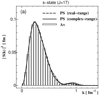
Figure 4: The squared moduli of breakup $S$-matrix elements as a function of $k$ at the grazing total angular momentum $J=17$ for $d$ + ⁵⁸Ni scattering at 80 MeV. The panel (a), (b), (c) and (d) shows the result for the s-state with, and the d-states with $L=15,17$ and 19 respectively. In each panel, the dashed (solid) line represents the result of the real-range (complex-range) Gaussian PS method. The step line is the result for the “exact” $S$-matrix element calculated the Av method.

In the real-range Gaussian PS method, a similar convergence is found, when the number of breakup channels, $N_{\rm PS}$, is 18 for both s- and d-waves. The number is even smaller when the complex-range Gaussian basis is taken: $N_{\rm PS}$ is 16 for s-wave and 17 for d-wave. The basis functions finally obtained have parameter sets $(a_{1}=1.0,a_{n}=30.0,n=30)$ for real-range Gaussian basis and $(a_{1}=1.0,a_{n}=20.0,2n=40,b=\pi/2)$ for complex-range one. For both of them $N_{\rm PS}$ is smaller than the number of basis functions. High-lying states with $k>k_{\rm max}$, which are obtained by diagonalizing $H_{\rm bc}$, do not affect the breakup $S$-matrix elements with $k<k_{\rm max}$, because the coupling potentials between the two $k$ regions are weak.

Figure 2 shows the discrete momenta $\hat{k}_{i\ell}$ translated from the eigenenergies $\epsilon_{i\ell}$ for the real- and complex-range Gaussian bases. One sees that for the real-range Gaussian basis, the discrete momenta are dense in the smaller $k$ region and sparse in the larger $k$ one. This distribution is not so effective in simulating the $k$ continuum, in the higher $k$ region in particular. For the complex-range Gaussian basis, on the other hand, the discrete momenta are distributed almost evenly. A similar sequence of the $\hat{k}_{i}$ is also seen for the case of the transformed harmonic oscillator basis of Ref. PS1 ; Perez . Such a sequence of $\hat{k}_{i}$ is close to that in the Av method. Thus, the complex-range Gaussian basis, as well as the transformed harmonic oscillator, is well suited for simulating the $k$ continuum in the entire region $0<k<k_{\rm max}$.

For the elastic $S$-matrix elements, both the real- and complex-range Gaussian PS methods well reproduce the “exact” one calculated with the Av method, as confirmed in Fig. 3 for the differential cross section. The three types of calculations, the real-range Gaussian PS, the complex-range Gaussian PS and the Av methods, yield an identical cross section at all scattering angles. Thus, both of the PS methods proposed here are useful for treating the breakup effects on the elastic scattering.

Figure 4 shows the result for breakup $S$-matrix elements at the grazing total angular momentum $J=17$, as a function of $k$. The real-range Gaussian PS method (dashed line) well simulates the exact solution calculated with the Av method (step line) in the lower $k$ region that corresponds to the main components of the breakup $S$-matrix elements, but inaccurate in the higher $k$ region around $k=0.8$ fm^-1. The deviation at higher $k$ stems from the fact that real-range Gaussian basis poorly reproduces the continuum breakup state $\Phi_{\ell}(k,r)$ at the higher $k$. Figure 4 shows that this problem can be solved by using the complex-range Gaussian basis (solid line) instead.

Figure 5: The same as in Fig. 3 but for ⁶Li; $k_{\rm max}$ is taken to be 2.0 fm^-1. The horizontal dashed line corresponds to the border momentum between the resonance and non-resonance parts used in the Av method.

Figure 6: Angular distribution of the elastic differential cross section (Rutherford ratio) for ⁶Li + ⁴⁰Ca scattering at 156 MeV. The results of the complex-range Gaussian PS method and the approximate treatment of the resonance of ⁶Li, i.e., the conventional Av method with the weight factor of Breit-Wigner type, are shown by the dashed and dash-dotted lines, respectively. The solid line is the “exact” solution calculated by the Av method with dense bins and the dotted line is the result of Watanabe model, i.e., without breakup effects.

IV.2 ⁶Li+⁴⁰Ca scattering at 156 MeV

Table 2: The same as in Table I but for $\alpha$ + ⁴⁰Ca at 104 MeV and $d$ + ⁵⁸Ca at 56 MeV.

system	$V_{0}$ (MeV)	$r_{0}$ (fm)	$a_{0}$ (fm)	$W_{0}$ (MeV)	$r_{\mathrm{W}}$ (fm)	$a_{\mathrm{W}}$ (fm)	$W_{\mathrm{D}}$ (MeV)	$r_{\mathrm{WD}}$ (fm)	$a_{\mathrm{WD}}$ (fm)
$\alpha$ + 40Ca	219.30	1.21	0.713	98.8	1.40	0.544	-	-	-
$d$ + 40Ca	75.470	1.20	0.769	2.452	1.32	0.783	9.775	1.32	0.783

Characteristic to this scattering, the projectile (⁶Li) has d-wave triplet resonance states ($3^{+},2^{+},1^{+}$). For simplicity, we neglect the intrinsic spin of ⁶Li, following Refs. CDCC-review1 ; sakuragi1 ; sakuragi2 . Then the projectile has only one d-wave resonance state with $\epsilon_{\rm res}=2.96$ MeV and $\Gamma=0.62$ MeV. Obviously the energy and the width do not reproduce experimental data, but at least the elastic cross section of ⁶Li is not affected much by the neglection of the spin Tanifuji .

In this scattering, the three-body system consists of deuteron, $\alpha$ and ⁴⁰Ca. The interactions between each pair of the constituents are the optical potential of $\alpha+^{40}$Ca scattering at 104 MeV HAU72 , that of $d+^{40}$Ca scattering at 56 MeV dCa , and $v_{\rm\alpha d}=v_{0}\exp\left[-(r/r_{0})^{2}\right]$ with $v_{0}=-74.19$ MeV and $r_{0}=2.236$ fm. Table II shows the parameters of the optical potentials.

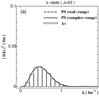
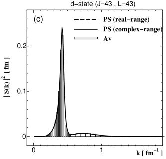
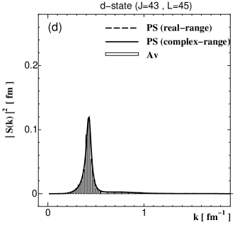
Figure 7: The same as in Fig. 4 but for ⁶Li + ⁴⁰Ca scattering at 156 MeV. The corresponding grazing total angular momentum is 43. The step line is the result of the Av method with dense bins. Note that the difference between the results of the real- and complex-range Gaussian PS methods is not visible since it is less than about 1%.

The model space sufficient for describing breakup processes in this scattering is $k_{\rm max}=2.0$ fm^-1 and $\ell_{\rm max}=2$; the model space is composed of two $k$-continua for $\ell=0$ and 2. Since there exists a resonance in $\ell=2$, the d-wave $k$-continuum is further divided in the Av method into the resonant part $[0<k<0.55]$ and the non-resonant part $[0.55<k<2.0]$. The $k$ continuum of $\Phi_{i,\ell=2}(k,r)$ in the resonant part varies rapidly with $k$. The Av method can simulate the rapid change by taking $f_{i,\ell=2}(k)=1$ with bins of an extremely small width. In fact clear convergence is found for both the elastic and the breakup $S$-matrix elements, when the resonance part is described by 30 bins and the non-resonance part of the d-wave and the s-wave $k$-continua by 20 bins. Another Av discretization, which has been widely used as a convenient prescription CDCC-review1 ; sakuragi1 ; sakuragi2 ; sakuragi4 ; Sakuragi , is also made for comparison, in which the resonance region is represented by a single state with the weight factor of Breit-Wigner type (9). The two sorts of Av discretization are compared with the real- and complex-range Gaussian PS methods. With the PS methods, convergence of the $S$-matrix elements is found with 21 s-wave breakup channels and 22 d-wave ones. The level sequence of the resulting discrete eigenstates is shown in Fig. 5 for both the basis functions. The level sequences have the same properties as in Fig. 2. The parameter sets of the basis functions, finally taken in the PS methods, are $(a_{1}=1.0,a_{n}=20.0,2n=40,b=\pi/2)$ for the complex-range Gaussian basis and $(a_{1}=1.0,a_{n}=30.0,n=30)$ for the real-range one.

Figure 6 shows the differential cross section of the elastic scattering. The result with the precise Av discretization based on dense bins, considered to be the “exact” solution, is denoted by the solid line. The dotted line represents the result of the Watanabe model, i.e., with no breakup channels. The conventional Av discretization, based on the weight factor of Breit-Wigner type (dash-dotted line), well describes the breakup effect, particularly at very forward angles ($\theta<20^{\circ}$), but deviates considerably from the “exact” solution at larger angles ($\theta>30^{\circ}$). The complex-range Gaussian PS discretization (dashed line) well reproduces the “exact” solution with a number of channels being suitable for practical use. The real-range Gaussian PS method gives just the same result as the complex-range one.

Figure 7 represents breakup $S$-matrix elements at grazing total angular momentum $J=43$. The real- and complex-range Gaussian PS discretization well reproduce the “exact” solution calculated by the Av discretization with dense bins. The results of the two PS methods turn out to coincide within the thickness of the line. The resonance peak can be expressed by only 8 (12) breakup channels in the complex-range (real-range) Gaussian PS method, while the corresponding number of breakup channels is 30 in the Av method, as mentioned above. Thus, one can conclude that the real- and complex-range Gaussian PS methods are very useful for describing not only non-resonant states but also resonant ones.

V Discussions on Four-body breakup reaction

In the past CDCC calculations the projectile was assumed to be a two-body system, dealing only with three-body breakup reactions. In this section, we investigate the applicability of CDCC to four-body breakup reactions of the projectile consisting of three particles, b+c+x (Fig. 8). The Av method needs the exact three-body wave functions being impossible to obtain. We can circumvent this problem with the present PS method; one can prepare an approximate complete set $\{\hat{\Phi}_{i\ell}\}$ by diagonalizing the Hamiltonian of the projectile in a space spanned by a set of basis functions of $L^{2}$ type. With $\{\hat{\Phi}_{i\ell}\}$ as the wave functions of the breakup channels, one can obtain an approximate total wave function $\Psi^{\rm CDCC}$ by solving CDCC equations (5). Inserting $\Psi^{\rm CDCC}$ into the exact form of breakup $T$-matrix elements in place of the exact total wave function, one reaches an approximate form:

$$T_{4}=\langle e^{i({\bf P}\cdot{\bf R}+{\bf k}\cdot{\bf r}+{\bf q}\cdot{\bf y})}|U_{4}|\Psi^{\rm CDCC}\rangle_{{\bf R,r,y}},$$ (20)

where $U_{4}$ is the sum of all interactions in the four-body system (A+b+c+x), ${\bf r}$ and ${\bf y}$ are and ${\bf k}$ and ${\bf q}$ are, respectively, two Jacobi coordinates of the three-body (b+c+x) system and momenta conjugate to them. The accuracy of Eq. (20) depends on how complete the set $\hat{\Phi}_{i\ell}$ is within the region $(0\leq r\leq r_{\rm max},0\leq y\leq y_{\rm max})$ which is important for the breakup process considered. An important advantage of the use of the real- and complex-range Gaussian bases is, as mentioned before, that analytic integrations over ${\bf r}$ and ${\bf y}$ can be done in Eq. (20), by expanding $U_{4}$ in terms of a finite number of Gaussian basis functions. This makes the derivation of $T_{4}$ feasible. Analyses based on this formulation are of much interest as a future work.

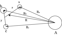
Figure 8: Illustration of a four-body (A+b+c+x) system. The projectile consists of b, c and x, and A is the target.

VI Summary

The method of continuum discretized coupled channels (CDCC) is an accurate method of treating three-body breakup processes, in which the discretization of the $k$ continuum is essential. In this paper, we propose the new method of pseudo-state (PS) discretization which can be used not only for virtual breakup processes in elastic scattering but also for breakup reactions. First we show that an accurate transformation from the discrete breakup S-matrix elements calculated with the PS method to continuous ones is possible, since the PS basis functions can form in the good approximation a complete set in the finite region of ${\bf r}$ and ${\bf k}$ which is important for the breakup processes. As bases satisfying the completeness, we propose the real- and complex-range Gaussian bases. Both bases can treat virtual breakup processes in the elastic scattering with high accuracy, i.e., with the error of calculated cross sections less than 1%. For breakup processes, the complex-range Gaussian basis is accurate throughout the entire region of the $k$ continuum. The real-range Gaussian basis also keeps a good accuracy for the dominant part of breakup $S$-matrix elements with the lower $k$, although it is partially inaccurate for the higher $k$ region. Thus, both bases can be used for realistic analyses of elastic scattering and projectile breakup reactions.

The present new PS method has at least two advantages over the widely used momentum bin average method. One is that it does not need the exact wave function of the projectile over the entire region of $r$. This is important from a theoretical point of view. The other advantage is that with the real- and complex-range Gaussian bases one can calculate all the coupling potentials semi-analytically, which is very useful in actual calculations. Furthermore, if the projectile has resonances in its excitation spectrum, the new method discretizes the complicated spectrum with a reasonable number of the basis functions, without distinguishing the resonance states from non-resonant continuous states. These advantages of the new method are extremely helpful, sometimes even essential, in applying CDCC to four-body breakup effects of unstable nuclei such as ⁶He and ¹¹Li. Actually, a CDCC analysis of four-body breakup effect on the ⁶He elastic scattering is in progress, and the result of the analysis will appear in a forthcoming paper.

References

- (1) M. Kamimura, M. Yahiro, Y. Iseri, Y. Sakuragi, H. Kameyama and M. Kawai, Prog. Theor. Phys. Suppl. 89, 1 (1986).
- (2) N. Austern, Y. Iseri, M. Kamimura, M. Kawai, G. H. Rawitscher and M. Yahiro, Phys. Reports. 154, 125 (1987).
- (3) M. Yahiro, N. Nakano, Y. Iseri and M. Kamimura Prog. Theor. Phys. 67, 1467 (1982).
- (4) M. Yahiro, Y. Iseri, M. Kamimura and M. Nakano, Phys. Lett. 141B, 19 (1984).
- (5) Y. Sakuragi and M. Kamimura, Phys. Lett. 149B, 307 (1984) .
- (6) Y. Sakuragi, Phys. Rev. C 35, 2161 (1987).
- (7) Y. Sakuragi, M. Kamimura and K. Katori, Phys. Lett. B205, 204 (1988).
- (8) Y. Sakuragi, M. Yahiro, M. Kamimura and M. Tanifuji, Nucl. Phys. A480, 361 (1988).
- (9) Y. Iseri, H, Kameyama, M. Kamimura, M. Yahiro and M. Tanifuji, Nucl. Phys. A490, 383 (1988).
- (10) Y. Hirabayashi and Y. Sakuragi, Phys. Rev. Lett. 69, 1892 (1992).
- (11) J. A. Tostevin, D. Bazin, B. A. Brown, T. Glasmacher, P. G. Hansen, V. Maddalena, A. Navin, and B. M. Sherrill, Phys. Rev. C 66, 024607 (2002); A. M. Moro, R. Crespo, F. Nunes, and I. J. Thompson, Phys. Rev. C 66, 024612 (2002) and references therein.
- (12) K. Ogata, M. Yahiro, Y. Iseri and M. Kamimura, Phys. Rev. C 67, R011602 (2003).
- (13) R. A. D. Piyadasa, M. Kawai, M. Kamimura and M. Yahiro, Phys. Rev. C 60, 044611(1999).
- (14) N. Austern, M. Yahiro and M. Kawai, Phys. Rev. Lett. 63, 2649 (1989); N. Austern, M. Kawai and M. Yahiro, Phys. Rev. C 53, 314 (1996).
- (15) M. Yahiro and M. Kamimura, Prog. Theor. Phys. 65, 2046 (1981); 65, 2051 (1981).
- (16) A. M. Moro, J. M. Arias, J. Gmez-Camacho, I. Martel, F. Prez-Bernal, R. Crespo and F. Nunes, Phys. Rev. C 65, 011602 (2002).
- (17) R. Y. Rasoanaivo and G. H. Rawitscher, Phy. Rev. C 39, 1709 (1989).
- (18) J. A. Tostevin, F. M. Nunes and I.J. Thompson, Phys. Rev. C 63, 024617 (2001).
- (19) M. Kamimura, Phys. Rev. A 38, 621 (1988).
- (20) E. Hiyama, Y. Kino and M. Kamimura, Progress in Particle and Nuclear Physics, 50, Issue 2 (2003), to be published.
- (21) F. D. Becchetti, Jr. and G. W. Greenlees, Phys. Rev. 182, 1190 (1969).
- (22) F. Prez-Bernal, I. Martel, J. M. Arias and J. Gmez-Camacho, Phys. Rev. A 63, 052111-1 (2001).
- (23) H.Ohnishi, M. Tanifuji, M. Kamimura, Y. Sakuragi and M. Yahiro, Nucl. Phys. A415, 271 (1984).
- (24) G. Hauser, R. Löhken, G. Nowicki, H. Rebel, G. Schatz, G. Schweimer and J. Specht, Nucl. Phys. A182, 1 (1972).
- (25) N. Matsuoka, H. Sakai, T. Saito, K. Hosono, M. Kondo, H. Ito, K. Hatanaka, T. Ichihara, A. Okihana, K. Imai and K. Nisimura, Nucl. Phys. A455, 413 (1986).