Mean first passage time for nuclear fission and the emission of light particles
Abstract
The concept of a mean first passage time is used to study the time lapse over which a fissioning system may emit light particles. The influence of the ”transient” and ”saddle to scission times” on this emission are critically examined. It is argued that within the limits of Kramers’ picture of fission no enhancement over that given by his rate formula need to be considered.
pacs:
24.75.+i, 05.60-k, 24.10.Pa, 24.60.DrIntroduction — Fission at finite thermal excitation is characterized by the evaporation of light particles and ’s. Any description of such a process must rely on statistical concepts, both with respect to fission itself as well as with respect to particle emission. For decades it has been customary to describe experiments in terms of particle FN-nat-par and fission widths, where the former, , is identified through the evaporation rate and the latter is given by the Bohr-Wheeler formula for the fission rate. Often in the literature this is referred to as the ”statistical model”. It was only in the 80’s that discrepancies of this procedure with experimental evidence was encountered: Sizably more neutrons were seen to accompany fission events than given by the ratio (for a review see e.g. pauthoe ). A possible enhancement of that ratio is found if the fission width is replaced by the of Kramers kram . In this seminal paper he pointed to the deficiency of the picture of Bohr and Wheeler in that it discards the influence of couplings of the fission mode to the nucleonic degrees of freedom. Such couplings will in general reduce the flux across the barrier, mainly because of the reduction of the energy in the fission degree of freedom which may then fall below the barrier. This is meant to represent the most likely path in a multidimensional landscape of shape degrees of freedom.
In Kramers’ picture this effect is realized through the presence of frictional and fluctuating forces (intimately connected to each other by the fluctuation dissipation theorem). Presently it is understood that Kramers’ ”high viscosity limit” applies (for a microscopic justification see hofrep ; hiry ), in which case the rate formula writes
| (1) |
Here, and stand for temperature and barrier height, for the frequency of the motion around the minimum at and for the dissipation strength at the barrier (at ) with being the friction coefficient and the inertia. For the sake of simplicity we will assume these coefficients not to vary along the fission path; otherwise the formula must be modified hiry . For vanishing dissipation strength (1) reduces to the Bohr-Wheeler formula (simplified to the case that the equilibrium of the nucleons can be parameterized by a temperature).
Commonly, formula (1) is derived (see e.g.scheuho ) in a time dependent picture solving the underlying Fokker-Planck equation for special initial conditions with respect to the time dependence of the distribution function FN-Kram-Smol . Their choice is intimately related to the picture of a compound reaction, in that the decay process is assumed to be independent of how the compound nucleus is produced. The latter in a sense represents a nucleus in a quasi-equilibrium such that the previous, pre-equilibrium stages need not be considered explicitly. This assumption is valid as long as the decay of that system takes longer than the equilibration time. To some large extent such a situation is indeed given at not too high excitations, as then the nucleons may stay inside this nuclear complex for a sufficiently long time. However, the circumstances are less clear with respect to the collective modes, in particular to the fission degree of freedom itself — which for large damping probably is among the slowest ones present. Whereas the corresponding kinetic momentum may safely be assumed to equilibrate sufficiently fast, this may not be so for the coordinate . Thus, assuming the system to be located initially around the supposedly pronounced ”ground state” minimum of the static energy at , the initial width in may still be at one’s disposal. In its true spirit the compound picture would suggest taking the equilibrium value, determined by the temperature and, in harmonic approximation, by the stiffness of the potential. Often, however, one starts with a sharp distribution of zero width. In any case, the current across the barrier needs some finite time to build up. This apparent delay of fission was interpreted graliwei ; bhagran as if there was the additional possibility of emitting light particles beyond the measure given by .
If besides collective motion also particle emission is studied explicitly in a time dependent picture, as done in the Langevin approach pobaridi ; mactheo , such an effect is included automatically. Problems arise, however, if one tries to imitate this delay in statistical codes which are in use for analyzing experimental results. Such codes apply static probabilities derived in time independent reaction theory. It is not obvious how this method may be reconciled with the picture of fission delay, the ”transient effect”. In the present note we like to shed some light on this problem by exploiting the concept of a mean first passage time (MFPT). Before we shall come to that we want to examine a little closer the time dependent case. We will concentrate on over-damped motion, as in this case the MFPT can be evaluated from an analytic formula. Moreover, for slow motion the transient time gets larger, such that the feature we want to discuss becomes even more obvious.
Time dependent current across the barrier — In the time dependent picture just described the boundary conditions in (and if present) are chosen to make sure that the distribution vanishes at infinity. Calculations of the current across the barrier then typically imply a behavior as exhibited in Fig.1. In all cases the asymptotic value of is seen to follow the law , shown by the fully drawn straight line. The differences at short times are due to the following different initial conditions:
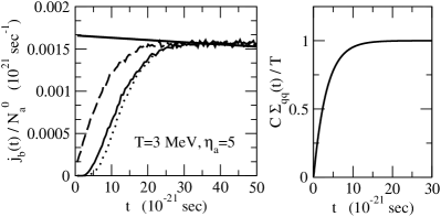
(i) For the dashed and dotted curves the system starts out of equilibrium in ; the dashed curve corresponds to the current at the barrier and the dotted one to that in the scission region , beyond which the fragments separate. The equilibrium is defined by the oscillator potential by which the around may be approximated.
(ii) For the fully drawn line the system starts at sharp. The obvious delay by about sec is essentially due to the relaxation of to the quasi-equilibrium in the well. This feature is demonstrated on the right by the -dependence of the width in (exhibited in terms of fluctuations of the potential energy ).
The figure clearly demonstrates remarkable uncertainties in the very concept of the ”transient effect”. First of all it is seen, that the ”transient” time , defined as the time the current needs to reach its asymptotic behavior, depends strongly on the initial conditions. Moreover, there is considerable arbitrariness in choosing time zero: If the calculation were repeated at some later time , the same features would be seen! In the end this is due to the very fact that the whole effect only comes about because in the initial distribution there are favorable parts for which it is easiest to reach the barrier. This is demonstrated in Fig.2. There, those points of the initial equilibrium are sampled which cross the barrier after some given time . On the right a sufficiently large was chosen such that greater parts of the initial distribution have ”fissioned”. As exhibited on the left, for the much shorter time , only a small fraction of points have succeeded in doing this, namely those which started close to the barrier (for under-damped motion also more favorite initial momenta would play a role, see HoIv-rauisch ; HoIv-MFPT-big ). The vast majority of particles is still waiting to complete the same motion but at later times! This aspect is important, not only for an understanding of the essentials of the concept of the MFPT vankampen ; gardiner-STM ; Risken , but also in respect to the evaporation of neutrons. Indeed, even for there is ample time for them to be emitted from inside the barrier.

The calculations have been performed by simulating the Langevin equations exploiting a locally harmonic approximation similar to that of scheuho ; hofrep for Kramers’ equation, for the following parameters: MeV, MeV, MeV and . The potential was constructed from two oscillators, one upright and one upside down, joined with a smooth first derivative.
The mean first passage time — Within a Langevin approach the concept of MFPT may be described as follows. Suppose that at particles start at the potential minimum . Because of the fluctuating force there will be trajectories which pass a certain exit point first at some time , the first passage time. The mean-FPT is defined by the average over all possibilities. In order to really obtain the mean first passage time the has to be removed from the ensemble once it has exited the interval at : the ”particle” can be said to be absorbed at (such that one may speak of an ”absorbing barrier”). As the potential is assumed to rise to infinity for , any motion to the far left will bounce back: the region acts as a ”reflecting barrier”. A calculation of the MFPT with the Langevin equation is shown in Fig.3 by the dashed double dotted curve and seen to be very close to the result obtained by exploiting special solutions of the Smoluchowski equation, which we want to address now.
Fortunately, the Smoluchowski approach allows one to derive an analytic formula for the vankampen ; gardiner-STM ; Risken . As one knows, the Smoluchowski equation represents that of Kramers for over-damped motion. For its solution the initial condition for the particles to start at is given by , which is identical to the one used for the fully drawn line of Fig.1. For constant friction and temperature one gets
| (2) |
This expression may be derived as follows: The probability of finding at time the particle still inside the interval is given by . Hence, the probability for it to leave the region during the time lapse from to is determined by , such that the average time becomes which turns into
| (3) | |||||
These formulas are associated to the special boundary conditions with respect to the
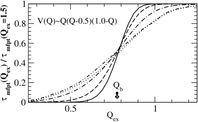
coordinate mentioned before, the reflecting barrier at and an absorbing barrier at . In particular for the latter feature it is not permitted to use in (3) the currents shown in Fig.1. Inserting them blindly would indeed lead to expressions for in which the appears FN-app-curr . This is in clear distinction to the correct form (2). Actually, the derivation of (2) involves proper solutions of that equation which is ”adjoint” to the Smoluchowski equation, and which describes motion backward in time. In Fig.3 we show the dependence of on as given by (2) calculated for a cubic potential. Evidently, the MFPT needed to reach the saddle at is exactly half the asymptotic value. The latter may be identified as the mean fission life time . For the typical conditions under which Kramers’ rate formula (1) is valid for overdamped motion, the identity of to the asymptotic value of the MFPT can be proven analytically gardiner-STM . Another remarkable feature seen in Fig.3 is the insensitivity of the MFPT to the exit point for small and large . Actually, in clear distinction to the transient time the MFPT is also insensitive to the starting point. This latter property shall be exhibited in a forthcoming paper HoIv-MFPT-big .

As a most interesting feature, the MFPT can be calculated also for cases of small barriers where Kramers’ formula does not apply. We show in Fig.4 results of evaluations of formula (2) for MeV as well as for a practically vanishing barrier. It is seen that even in the latter case the reaches a plateau for sufficiently large . This asymptotic value, however, is no longer determined by . Nevertheless, the seems to be long enough for neutrons to be evaporated before scission. This may be seen as follows. The neutron width typically is of the order of MeV (for medium heavy nuclei pobaridi ). According to hiry the roughly increases linearly in , being about /MeV at MeV and about /MeV at MeV. Taking the values of from the right part of Fig.4 and close to the plateau one gets a width of the order of MeV, and thus comparable to the neutron width. Fig.4 also shows that a small increase of the barrier by 1 MeV enlarges the drastically. Discussion — It should be evident from the previous discussion that in the very concept of the MFPT there is no room for a transient effect. After all, formula (2) is based on exact solutions of the transport equation which satisfy the same initial condition as those used for the plots in Fig.1 — albeit different boundary conditions in coordinate space. Moreover, as exhibited in Fig.2 the evaluation of the MFPT takes into account an average over all initial points, as is warranted by the definition of the MFPT through the probability distribution . Contrasting this feature, and as outlined in the second section, the transient effect only represents a minor part of the initial population, namely that one which reaches the barrier first. Discarding the rest implies ignoring the many particles which are still moving inside the barrier for times typically much longer than . Hence, neutrons from deformations corresponding to that region may not only be emitted within but within , which turns out to be just half of the total fission time . Of course, this discussion shows that it is also not correct to argue in favor of ”additional” neutrons which might be emitted within the saddle to scission time introduced in hofnix . As one may guess from Fig.3, like the , the does not appear to be in accord with the MFPT either: The time the fissioning system stays together is not determined by motion in the immediate neighborhood of the barrier. On average it takes half the full decay time to move beyond the to the at which the reaches its plateau value.
These findings suggest that one simply estimates the emission rate of neutrons over fission from the ratio — provided one may trust the potential to be of the simple form underlying the rate formula (1). Anything else does not seem to be in accord with an appropriate application of Kramers’ or Smoluchowski’s equations. This does not rule out other, complementary effects which originate in more complicated situations. For instance, in case that in the scission region the potential becomes flat again or even develops a minimum the system is forced to stay there longer than given by the of eq.(1) — implying additional time for evaporating neutrons. Likewise it is conceivable that the initial stage of the whole reaction is to be described with a different transport model. Such modifications are already suggested when the average neutron emission time becomes comparable to or even smaller than the relaxation time for the nucleonic degrees of freedom as a whole. Transport equations are justified only if this is the smallest time scale present, in comparison to both neutron emission as well as to collective motion. The turns out to be of the order of sec, no matter whether it is estimated within linear response theory with collisional damping or within a random matrix approach (see hofrep ). Applying the Weisskopf estimate for the neutron emission time (or modified versions of it) pobaridi at large temperatures one easily gets values of of the order of or smaller than . This reflects a situation of pre-equilibrium rather than that assumed in the quasi-static picture necessary for the application of Fokker-Planck equations. In conclusion we may say that deviations of experimental results from the standard value of ought perhaps to be understood as a strong indication of the relevance of these complementary effects, which unfortunately have for the most part been unconsidered. This might require one to re-examine analyzes of experiments which over the past decade or so have followed the conventional line.
The authors benefitted greatly from a collaboration meeting on ”Fission at finite thermal excitations” in April, 2002, sponsored by the ECT* (’STATE’ contract). One of us (F.A.I.) would like to thank the Physik Department of the TUM for the hospitality extended to him.
References
- (1) To simplify the discussion we will not distinguish the nature of the ”particles” and in this sense include ’s in this notation.
- (2) P. Paul and M. Thoennessen, Ann. Rev. Part. Nucl. Sci. 44, 65 (1994).
- (3) H.A. Kramers, Physica 7, 284 (1940).
- (4) H. Hofmann, Phys. Rep. 284 (4&5), 137-380 (1997).
- (5) H. Hofmann, F.A. Ivanyuk, C. Rummel and S. Yamaji, Phys. Rev. C 64, 054316 (2001).
- (6) F. Scheuter et al., Nucl. Phys. A 394, 477 (1983).
- (7) For Kramers’ equation this involves the coordinate and a momentum . The latter is absent in the Smoluchowski equation for overdamped motion.
- (8) P. Grangé et al. Phys. Rev. C 27, 2063 (1983).
- (9) K. H. Bhatt et al., Phys. Rev. C 33, 954 (1986).
- (10) K.Pomorski et al., Nucl. Phys. A 605, 87 (1996).
- (11) K.Pomorski et al., Nucl. Phys. A 679, 25 (2000); P.Fröbrich and I.I.Gontchar, Phys.Rep. 292, 131 (1998); Y.Aritomo et al., Phys. Rev. C 55, 1011 (1997).
- (12) H. Hofmann and F.A. Ivanyuk, Proc. Symp. Nuclear Clusters, Rauischholzhausen, Germany, 5-9 August 2002, 2003 EP Systema, Debrecen (Hungary)” with the ISBN 963 206 299 X; see nucl-th/0210004.
- (13) H. Hofmann and F.A. Ivanyuk, to be published .
- (14) N.G. van Kampen, Stochastic processes in physics and chemistry (North-Holland, Amsterdam, 2001).
- (15) C.W. Gardiner, Handbook of stochastic methods (Springer, Berlin, 2002).
- (16) H. Risken, The Fokker-Planck-Equation (Springer, Berlin, 1989).
- (17) Approximating the form of the current by one would falsely get .
- (18) H. Hofmann and J.R. Nix, Phys. Lett. B 122, 117 (1983).