Modified two-potential approach to tunneling problems

Abstract

One-body quantum tunneling to continuum is treated via the two-potential approach, dividing the tunneling potential into external and internal parts. We show that corrections to this approach can be minimized by taking the separation radius inside the interval determined by simple expressions. The resulting modified two-potential approach reproduces the resonance’s energy and the width, both for narrow and wide resonances. We also demonstrate that, without losing its accuracy, the two-potential approach can be modified to a form resembling the R-matrix theory, yet without any uncertainties related to the choice of the matching radius.

I Introduction

The quantum mechanical tunneling through a classically forbidden region is an ubiquitous phenomenon in physics, which has been extensively studied since the early days of quantum mechanics. In 1927, Hund Hund was the first to point out the possibility of “barrier penetration” between two discrete states. In the same year, Nordheim Nordheim considered the case of tunneling between continuum states. Subsequently, Oppenheimer Oppy performed a calculation of the rate of ionization of the hydrogen atom, and Gamow, Gamow Gurney and Condon Gurney explained alpha decay rates of radioactive nuclei in terms of the tunneling effect.

While the semi-classical treatment of tunneling turned out to be very successful in many applications, the numerical calculation offers very little insight into the physical process. In addition, the validity of the standard WKB formula is rather restricted. Other methods, although more accurate, contain various uncertainties. For example, the results of the commonly used R-matrix theory lane are often sensitive to the choice of the matching radius humb ; Arima , and the theoretical error is difficult to estimate.

The treatment of the tunneling problem can be essentially simplified by reducing it to two separate problems: a bound state problem and a non-resonant (scattering) state problem. This can be done consistently in the two-potential approach (TPA) gk ; g ; g1 (see also Refs. jrb ; tore ), representing the barrier potential as a sum of the “inner” and the “outer” terms, containing only bound and only scattering states, respectively. This approach not only provides better physical insights than many other approximations but it is also simple and accurate.

In this paper we propose further developments and a modification of the TPA, and present a detailed comparison of this approach with the results of numerical calculations based on the Gamow-state (resonant-state) formalism. The resulting analytical expressions are easy to interpret and they can be straightforwardly extended to the non-spherical case.

The paper is organized as follows. In Sect. II, the TPA is briefly described. Section III deals with the quantal correction terms to the TPA. The minimization of these terms prescribes unambiguously the “window” for the separation radius that divides the original barrier potential into inner and outer terms. In this case, by considering examples of wide and narrow nuclear resonances, we demonstrate that the TPA yields results which are practically the same as those of the resonant-state calculation. In Sec. IV, we present a modification of the TPA. The resulting expressions resemble those of the R-matrix theory, yet without any uncertainties related to the matching radius, see Sec. V. Finally, the summary of our work is contained in Sec. VI.

II Two-potential approach

Consider a quantum well $V(r)$ with a barrier, which contains a quasi-stationary state at the $E_{res}$.

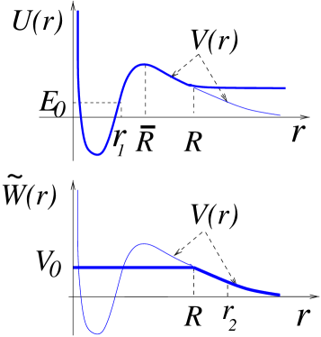
Figure 1: The “inner” ($U$; top) and the “outer” ($\tilde{W}$; bottom) parts of the potential $V(r)$ defined as in Eqs. (1) and (2), respectively. The separation radius $R$ is chosen well inside the barrier. The energy of the metastable state is $E_{0}$ and $V_{0}$=$V(R)$. The barrier radius is denoted by $\bar{R}$ and $r_{1,2}$ are the classical turning points.

The coordinate space can be divided into two regions, the “inner” region, $0<r<R$, and the “outer” region, $r$$>$$R$, where $R$ is taken inside the barrier (see Fig. 1). Accordingly, one can introduce the two auxiliary potentials: the inner potential

$$U(r)=\left\{\begin{array}[]{ll}V(r)&{\mbox{for}}~{}~{}r\leq R\\ V(R)=V_{0}&{\mbox{for}}~{}~{}r>R\end{array}\right.$$ (1)

and the outer potential

$$\tilde{W}(r)=\left\{\begin{array}[]{ll}V_{0}&{\mbox{for}}~{}~{}r\leq R\\ V(r)&{\mbox{for}}~{}~{}r>R\end{array}\right..$$ (2)

The inner potential contains a bound state, $\Phi_{0}(r)$ ($E$=$E_{0}$), representing an eigenstate of the “inner” Hamiltonian $H_{0}=K+U(r)$, where $K=-\nabla^{2}/2m$ is the kinetic energy term ($\hbar$=1). One can demonstrate g that the energy and the width of the quasi-stationary state, associated with the complex-energy poles of the total Green’s function $G(E)=(E-K-V)^{-1}$, are obtained from the following equation

$$E=E_{0}+\langle\Phi_{0}|W|\Phi_{0}\rangle+\langle\Phi_{0}|W\tilde{G}(E)W|\Phi_{0}\rangle\,.$$ (3)

Here $W(r)=\tilde{W}(r)-V_{0}$, and the Green’s function $\tilde{G}$ is given by

$$\tilde{G}(E)=G_{0}(E)\left[1+\tilde{W}\tilde{G}(E)\right],$$ (4)

where

$$G_{0}(E)=\frac{1-\Lambda}{E+U_{0}-K-U},\;\;\;\;\Lambda=|\Phi_{0}\rangle\langle\Phi_{0}|.$$ (5)

The resonance energy $E_{\rm res}=\Re(E)$ and the width $\Gamma=-2\Im(E)$ of a quasi-stationary state obtained from Eq. (3) are independent of the choice of the separation radius $R$.

Equation (3) can be solved iteratively by using the standard Born series for the Green’s function $\tilde{G}$, i.e. by expanding $\tilde{G}$ in powers of $G_{0}$. Yet, the corresponding expansion for the quasi-stationary state energy converges very slowly. For that reason, we proposed g a more efficient expansion scheme in which $\tilde{G}$ is expanded in powers of the Green’s function $G_{\tilde{W}}(E)=(E-K-\tilde{W})^{-1}$, corresponding to the outer potential $\tilde{W}$. From Eq. (4) it immediately follows that

$$\tilde{G}=G_{\tilde{W}}+G_{\tilde{W}}\left(U-U_{0}\right)\tilde{G}-\tilde{G}_{\tilde{W}}\Lambda\left(1+\tilde{W}\tilde{G}\right)\,,$$ (6)

Iterating Eq. (6) in powers of $G_{\tilde{W}}$ and then substituting the result into (3), one finds the desirable perturbative expansion for the energy and the width of the resonance. By truncating this series, one obtains the following first-order relation valid for the isolated metastable state:

$$E=E_{0}+\langle\Phi_{0}|W|\Phi_{0}\rangle+\langle\Phi_{0}|WG_{\tilde{W}}(E)W|\Phi_{0}\rangle.$$ (7)

The above equation can be solved iteratively for $E=E_{r}-i\Gamma/2$ by assuming that the energy shift $\Delta=E_{r}-E_{0}$ and the width $\Gamma$ are small compared to $E_{0}$ and $V_{0}-E_{0}$. In such a case, one can put $G_{\tilde{W}}(E)\approx G_{\tilde{W}}(E_{0})$, thus reducing Eq. (7) to

$$E=E_{0}+\langle\Phi_{0}|W|\Phi_{0}\rangle+\langle\Phi_{0}|WG_{\tilde{W}}(E_{0})W|\Phi_{0}\rangle.$$ (8)

By using the Schrödinger equation for $G_{\tilde{W}}$ one finally obtains the TPA expressions gk ; g for the width $\Gamma$ and for the energy shift $\Delta=E_{\rm res}-E_{0}$ of the quasi-stationary state:

$$\Gamma\!\! = \!\frac{1}{mk}\left[\Phi_{0}(R)\chi^{\prime}_{k}(R)-\Phi^{\prime}_{0}(R)\chi_{k}(R)\right]^{2},$$ (9)

$$\Delta\!\! = \!-\frac{\Phi^{2}_{0}(R)}{2mk}\left[\alpha\chi_{k}(R)+\chi^{\prime}_{k}(R)\right]\left[\alpha\tilde{\chi}_{k}(R)+\tilde{\chi}^{\prime}_{k}(R)\right],$$ (10)

where $k=\sqrt{2mE_{0}}$, $\alpha=\sqrt{2m(V(R)-E_{0})}$, $\tilde{\chi}_{k}(r)=\Re({\chi_{k}^{(+)}(r)})$, and $\chi_{k}$ ($\chi_{k}^{(+)}$) stands for the irregular (outgoing) solution of the Schrödinger equation for the outer potential.

It follows from Eqs. (9) and (10) that both $\Gamma$ and $\Delta$ are given in terms of bound and scattering state wave functions. Thus TPA essentially simplifies the treatment of tunneling, because the standard approximation schemes can be used for evaluation of $\Phi_{0}$ and $\chi_{k}$. For instance, by applying the semi-classical approximation, one obtains the improved Gamow formula for $\Gamma$ gk ; g , which is useful for different applications buck ; nazar . In particular, an extension of Eqs. (9) and (10) to the multi-dimensional case can be found in Ref. g1 .

III Corrections to TPA and the choice of the separation radius

The accuracy of Eqs. (9) and (10) can be determined by evaluating the leading correction terms. There are two types of corrections to TPA: (a) those due to the replacement of $\tilde{G}$ by $G_{\tilde{W}}$ in Eq. (3) leading to Eq. (7), and (b) those due to the replacement of $G_{\tilde{W}}(E)$ by $G_{\tilde{W}}(E_{0})$ in Eq. (7) leading to Eqs. (9), (10). The correction terms of the first type, $(\Delta\Gamma)_{1}$, can be obtained by iterating (6). One finds from the first iteration g :

$${(\Delta\Gamma)_{1}\over\Gamma}\simeq{mV^{\prime}(R)\over 16[2m(V_{0}-E_{0})]^{3/2}}.$$ (11)

Equation (11) might suggest that an optimal choice of the separation radius corresponds to $V^{\prime}(R)=0$, i.e., the maximum of $V(r)$. However, it has been demonstrated numerically nazar ; talou that if the top of the barrier is close to the closing potential, such a choice is not optimal, since in this case Eqs. (9) and (10) become less accurate. The reason is that the energy shift $\Delta$ becomes appreciable so that (7) cannot be replaced by (8).

This can be illustrated by considering a square-well potential discussed in Ref. erich : $V(r)=l(l+1)/2mr^{2}-U_{0}$ for $r<R_{1}$, and $V(r)=l(l+1)/2mr^{2}$ for $r\geq R_{1}$, where the top of the barrier coincides with the closing potential (see Fig. 2).

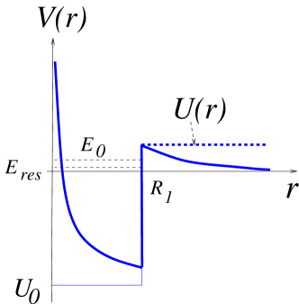
Figure 2: Metastable state in the square-well potential of Ref. erich . The potential parameters ($U_{0}$=-51.6 MeV and $R_{1}$=6 fm) correspond to a P-wave resonance at $E_{\rm res}=1$ keV and $\Gamma$ =55.9 eV. The bound state in the potential $U(r)$ lies at $E_{0}$=275 keV. The top of the centrifugal barrier is at $V(R_{1})$=1.16 MeV.

For a P-wave resonance, the numerical calculation gives $E_{\rm res}=1$ keV and $\Gamma=55.9$ eV erich . Now we apply the TPA by taking the separation radius at the boundary, $R=R_{1}$. The corresponding inner potential $U(r)$ has a bound state at $E_{0}$=275 keV. However, the corresponding energy shift, $\Delta$=$-$300 keV, is of the same order of magnitude as the energy $E_{0}$ of the bound state. Consequently, the replacement of $G_{\tilde{W}}(E)$ by $G_{\tilde{W}}(E_{0})$ in (7) leads to large corrections to the resonance energy and the width so that Eqs. (9) and (10) cannot be used.

Let us estimate the correction term $(\Delta\Gamma)_{2}=\Gamma(E_{0}+\Delta)-\Gamma(E_{0})$ due to such a replacement. One can use the semi-classical Gamow formula, $\Gamma\propto\exp(-2\int_{r_{1}}^{r_{2}}|p(r)|dr$, with $r_{1}$ and $r_{2}$ being the inner and outer classical turning points, respectively, and $|p(r)|=\sqrt{2m[V(r)-E_{0}]}$. Approximating $V(r)$ for $r_{1}<r<r_{2}$ by the inverted harmonic oscillator, one obtains

$${(\Delta\Gamma)_{2}\over\Gamma}\simeq\Delta\int_{r_{1}}^{r_{2}}{\sqrt{2m}\over\sqrt{V(r)-E_{0}}}dr\approx\pi{\sqrt{2m}(r_{2}-r_{1})\over 2\sqrt{\bar{V}-E_{0}}}\Delta\ ,$$ (12)

where $\bar{V}$= max $V(r)$ and $\Delta$ is is given by Eq. (10).

Thus, in order to reduce the correction term $(\Delta\Gamma)_{2}$, one needs to minimize the energy shift $\Delta$. It follows from (10) that $\Delta$ can be strongly suppressed by taking the separation radius $R$ deeply inside the barrier. Indeed, Eq. (10) contains a product of regular and irregular wave functions, which do not vary considerably under the barrier. However, the factor $|\Phi_{0}(R)|^{2}$ decays exponentially with $R$. Therefore, by taking the separation radius $R$ far away from the boundary, $R\gg r_{1}$, one finds that $\Delta\to 0$, and $E_{0}\to E_{\rm res}$. As a result, (7) can be replaced by (8), leading to Eqs. (9) and (10).

To illustrate this point, let us again consider the example of a P-wave resonance discussed above. By taking the separation radius $R>R_{1}$, we readily find that $\Delta\to 0$ as $R-R_{1}$ increases, and $E_{0}\to E_{\rm res}$= 1 keV. The resulting value of $\Gamma$=55.3 eV is very close to the Gamow-state value of the resonance width. The separation radius $R$ cannot be chosen too close to the outer classical turning point since in such a case $V(R)\to E_{0}$ and the correction term (11) becomes important. In fact, Eqs. (11) and (12) define the lower and upper limits of $R$.

In the following, we discuss the TPA results for proton and neutron resonances in the realistic average nuclear potential. The approximate TPA expressions are compared to the resonant states results obtained using the GAMOW code gamow .

III.1 Comparison with Gamow-state calculations

Consider single-nucleon resonances in the Woods-Saxon (WS) potential $V_{WS}(r)$ represented by a sum of central, spin-orbit, centrifugal, and Coulomb terms. Here, we apply the parametrization of Ref. nazar , namely: $R_{0}$=1.17A^1/3 fm, $a=0.75$ fm for the central term, and $U^{so}_{0}=0.2U_{0}$ and $R^{so}_{0}=1.01$A^1/3 for the spin-orbit potential. We calculate $\Delta$ and $\Gamma$ according to Eqs. (9) and (10) by varying the separation radius $R$ inside the barrier, starting with the barrier radius, $\bar{R}$, corresponding to the maximum of $V(r)$.

Table 1: TPA calculations for the $0h_{11/2}$ and $2s_{1/2}$ proton resonances with energy $E_{\rm res}$=1.5 MeV in a WS potential. The calculated widths $\Gamma_{\rm{TPA}}$ and the corresponding corrections (11) and (12) are shown relative to $\Gamma_{\rm TPA}$ for several values of the separation radius $R$. The actual accuracy of the TPA, $\Delta\Gamma/\Gamma$, is given in the last column. If the correction is marked zero, it means that it is below 0.1%.

$R-\bar{R}$	$\Delta$	$\Gamma_{\rm{TPA}}$	$\underline{(\Delta\Gamma)_{1}}$	$\underline{(\Delta\Gamma)_{2}}$	$\underline{(\Delta\Gamma)}$
(fm)	(keV)	(MeV)	$\Gamma_{TPA}$	$\Gamma_{TPA}$	$\Gamma$
$0h_{11/2}$ Gamow state: $E_{\rm res}$=1.5 MeV, $\Gamma$ =4.918 E-18 MeV
0	-1.9	4.931 E-18	0	-1%	-0.3%
1.59	-0.27	4.919 E-18	0	-0.15%	0
4.28	-5.0 E-3	4.919 E-18	0	0	0
$2s_{1/2}$ Gamow state: $E_{\rm res}$=1.5 MeV, $\Gamma$ =6.695 E-14 MeV
0	-3.3	6.727 E-14	0	-2.3%	-0.5%
3.48	-0.11	6.709 E-14	0	-0.1%	-0.2%
8.05	-1.2 E-3	6.746 E-14	-0.7%	0	-0.7%

We begin with the high-$\ell$ narrow proton resonance 0h_11/2. The parameters of the WS potential are appropriate for ¹⁴⁷Tm, which is a proton emitting nucleus. The potential depth, $U_{0}$=$-$61.8823 MeV, was adjusted to the energy $E_{\rm res}$=1.5 MeV. The resulting barrier radius is $\bar{R}$=8.54 fm ($V(\bar{R})$=17.44 MeV) and the inner and outer turning points are $r_{1}$=6.33 fm and $r_{2}$=71.15 fm, respectively. Since $E_{\rm res}\ll V(\bar{R})$, the calculated 0h_11/2 resonant state has a very small width, $\Gamma$=4.918 10^-18 MeV. The results of TPA calculations are shown in Table I for different values of $R\geq\bar{R}$, together with the corresponding correction terms to TPA: $(\Delta\Gamma)_{1}/\Gamma_{\rm TPA}$ (11) and $(\Delta\Gamma)_{2}/\Gamma_{\rm TPA}$ (12). Table I also displays the actual accuracy of the TPA, $(\Delta\Gamma)/\Gamma$, where $(\Delta\Gamma)=\Gamma-\Gamma_{\rm TPA}$. Since $\bar{R}>r_{1}$, the energy shift $\Delta$ is small for $R=\bar{R}$. Therefore, the results of TPA are in a good agreement with the resonant-state calculations already for $R=\bar{R}$. Next we consider the low-$\ell$, broader 2s_1/2 resonance at $E_{\rm res}$=1.5 MeV, which is considerably closer to the top of the barrier $V(\bar{R})=9.43$ MeV ($\bar{R}$=9.34 fm). As shown in Table I, also in this case $\Gamma_{\rm{TPA}}$ nicely agrees with the numerical result, and the accuracy of the TPA is well estimated by Eqs. (11) and (12).

Table 2: Same as in Table 1, except for the neutron $0i_{13/2}$ and $1f_{5/2}$ resonances.

$R-\bar{R}$	$\Delta$	$\Gamma_{\rm{TPA}}$	$\underline{(\Delta\Gamma)_{1}}$	$\underline{(\Delta\Gamma)_{2}}$	$\underline{(\Delta\Gamma)}$
(fm)	(keV)	(MeV)	$\Gamma_{TPA}$	$\Gamma_{TPA}$	$\Gamma$
$0i_{13/2}$ Gamow state: $E_{\rm res}$=1 MeV, $\Gamma$ =1.834 E-6 MeV
0	-11.9	1.869 E-6	0	-3%	-1.9%
3.45	-0.47	1.844 E-6	-1.2%	-0.1%	-0.5%
5.96	-6.1 E-2	1.847 E-6	-1.5%	0	-0.7%
$1f_{5/2}$ Gamow state: $E_{\rm res}$=1 MeV, $\Gamma$ =9.271 E-2 MeV
0	-109	1.227 E-1	0	-25%	-32%
2.05	-51.4	1.089 E-1	-10.1%	-12%	-17%
4.05	-7.2	9.876 E-2	-12%	-1.7%	-6.5%
4.57	+2.7	9.408 E-2	-17%	+0.6%	-1.5%

Table II displays the TPA results for the 0i_13/2 and 1f_5/2 neutron resonances in ¹³³Sn at an energy $E_{\rm res}$=1 MeV. Here $\Gamma$ is much larger due to the absence of the Coulomb barrier. As in the proton case, there is very good agreement with numerical calculations, provided that $R$ is taken far away from the turning points, inside the window determined by (11) and (12), and the results of TPA weakly depend on the separation radius $R$. This suggests that the separation radius can be eliminated altogether from the TPA expressions. As demonstrated in the following section one can indeed modify the TPA in such a way.

IV Modified Two-Potential Approach

A tunneling potential can always be written as a sum of attractive and repulsive parts, $V(r)=V_{att}(r)+V_{rep}(r)$, where $V_{rep}(r)$ becomes dominant at distances beyond the barrier radius (see Fig. 3).

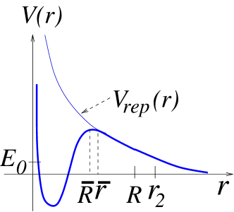
Figure 3: For $r>\bar{r}$ the tunneling potential $V(r)$ can be approximated by its repulsive part $V_{rep}(r)$. $R$ and $r_{2}$ denote the TPA separation radius and the outer turning point ($V(r_{2})=E_{0}$), respectively.

Therefore, starting with some radius $\bar{r}$, the total potential $V(r)$ can be well approximated by the repulsive component only. The value of $\bar{r}$ should be chosen in such a way that the attractive (e.g., nuclear) part can disregarded with a desired accuracy $\eta\ll 1$:

$$|1-V_{rep}(r)/V(r)|\leq\eta~{}~{}~{}~{}~{}~{}{\mbox{for}}~{}r\geq\bar{r}\,.$$ (13)

For instance, in the case of a square-well potential of Fig. 2, Eq. (13) is satisfied for any $\eta$ provided that $\bar{r}$$>$$R_{1}$. In most cases, the attractive potential rapidly decreases beyond the barrier radius, so that $\bar{r}$ is closer to $\bar{R}$ than to the separation radius $R$ in the TPA (cf. Fig. 3).

Usually, the repulsive part $V_{rep}(r)$ is well known, as well as the two linearly independent (regular and irregular) solutions $F_{k}(r)$ and $G_{k}(r)$ of the corresponding Schrödinger equation. For instance, if $V_{rep}(r)$ is a sum of Coulomb and centrifugal potentials, then $F_{k}(r)$ and $G_{k}(r)$ are the standard Coulomb functions. This implies that any solution of the Schrödinger equation with the potential $V(r)$ can be written for $r>\bar{r}$ as the linear combination of $F_{k}(r)$ and $G_{k}(r)$.

Consider the bound-state wave function $\Phi_{0}(r)$ of the inner potential $U(r)$ of Eq. (1). Since $U(r)\simeq V_{rep}(r)$ for $\bar{r}\leq r\leq R$, $\Phi_{0}(r)$ can be expanded in this region as

$$\Phi_{0}(r)=c_{1}G_{k}(r)+c_{2}F_{k}(r)\,,$$ (14)

where $k=(2mE_{0})^{1/2}$. The coefficients $c_{1,2}$ and the energy $E_{0}$ are obtained from matching of the logarithmic derivatives at $r=\bar{r}$ and $r=R$:

$${c_{1}G^{\prime}_{k}(R)+c_{2}F^{\prime}_{k}(R)\over c_{1}G_{k}(R)+c_{2}F_{k}(R)} = -|p(R)|,$$ (15a)

$${c_{1}G^{\prime}_{k}(\bar{r})+c_{2}F^{\prime}_{k}(\bar{r})\over c_{1}G_{k}(\bar{r})+c_{2}F_{k}(\bar{r})} = {\Phi^{\prime}_{0}(\bar{r})\over\Phi_{0}(\bar{r})}.$$ (15b)

Note that $\Phi_{0}(r)\propto\exp[-|p(R)|(r-R)]$, for $r>R$. Solving Eqs. (15) one easily finds

$${\Phi_{0}^{\prime}(\bar{r})\over\Phi_{0}(\bar{r})}={G^{\prime}_{k}(\bar{r})\over G_{k}(\bar{r})}\left[{1+\alpha a_{k}^{-1}-f_{1}(1+\tilde{a}_{k}^{-1})\over 1+\alpha a_{k}^{-1}-f_{2}(1+\tilde{a}_{k}^{-1})}\right]\ ,$$ (16)

where $\alpha=|p(R)|$, $a_{k}={F^{\prime}_{k}(R)/F_{k}(R)}$, $\tilde{a}_{k}={G^{\prime}_{k}(R)/G_{k}(R)}$, and

$$f_{1}={G^{\prime}_{k}(R)F^{\prime}_{k}(\bar{r})\over F^{\prime}_{k}(R)G^{\prime}_{k}(\bar{r})},~{}~{}~{}f_{2}={G^{\prime}_{k}(R)F_{k}(\bar{r})\over F^{\prime}_{k}(R)G_{k}(\bar{r})}.$$ (17)

The wave functions $F_{k}(r)$ and $G_{k}(r)$ are of the same order of magnitude in the asymptotic region, $r\gg r_{2}$. However, in the classically forbidden region the regular wave function exponentially decreases and the irregular one exponentially increases with decreasing $r$. Using the semi-classical approximation, one can estimate $G_{k}(R)F_{k}(\bar{r})\sim\exp[-\int_{\bar{r}}^{R}|p(r)|dr]$. Therefore, the coefficients $f_{1,2}$ are of the order of $\exp[-\alpha(R-\bar{r})]$, so the corresponding terms $f_{1,2}(1+\tilde{a}_{k}^{(-1)})$ in Eq. (16) are exponentially suppressed and can be neglected. As a result, the matching condition (16) can be written as

$${\Phi^{\prime}_{0}(\bar{r})\over\Phi_{0}(\bar{r})}={G^{\prime}_{k}(\bar{r})\over G_{k}(\bar{r})}\,.$$ (18)

The above equation constitutes the MPTA condition for the resonance energy $E_{\rm res}=E_{0}$. In contrast to Eq. (16), the relation (18) does not exhibit any explicit $R$-dependence. Consequently, there is no need to evaluate the bound-state wave function at large values of $R$ well inside the barrier. Note also that for a narrow resonance the irregular wave function $G_{k}(r)$ is proportional to the real part of the outgoing (Gamow) solution:

$$\Psi^{out}_{k_{res}}(r)\propto G_{k_{res}}(r)+iF_{k_{res}}(r)=O_{k_{res}}(r),$$ (19)

with complex $k_{res}=k-i\gamma$ and $k_{res}^{2}=2m(E_{res}-i\Gamma/2)$. Since for small $\Gamma$ and $\gamma$ the imaginary parts of $k_{res}$ and $G_{k_{res}}(r)$ can be neglected, $k_{res}\approx k$ and $G_{k_{res}}(r)\approx G_{k}(r)$ (also for the outgoing Coulomb wave function $O_{k_{res}}(r)=O_{k}(r)$). In this case Eq. (18) represents the matching condition for the inner (bound state) wave function with the real part of the non-normalized outgoing wave. If the imaginary parts are not negligible, Eq. (18) can be still interpreted in terms of the standing-wave boundary condition at $\bar{r}$, which means that the scattering phase shift is $\pi/2$. The requirement that the phase shift is equal to $\pi/2$ represents an alternative definition for the position of a resonance in the absence of a non-resonant phase shift.

Consider now Eq. (9) for the width. Since $R>\bar{r}$, the outer wave function $\chi_{k}(r)$ in the region $r\geq R$ can be represented by the linear combination of the regular and irregular solutions of $V_{rep}(r)$, and the corresponding coefficients in the linear combination of $F_{k}(r)$ and $G_{k}(r)$ are directly related to the (non-resonant) scattering phase shift for the outer potential $\tilde{W}(r)$. One easily finds

$$\chi_{k}(r)=\cos\delta_{k}\ F_{k}(r)+\sin\delta_{k}\ G_{k}(r)~{}~{}~{}{\mbox{for}}~{}~{}r\geq R\,,$$ (20)

where the phase shift $\delta_{k}$ is obtained from matching of logarithmic derivatives at the separation radius $R$:

$$\tan\delta_{k}=-{F_{k}(R)\over G_{k}(R)}\left({a_{k}-\alpha\over\tilde{a}_{k}-\alpha}\right)\ .$$ (21)

Here we neglected the terms $\sim\exp(-2\alpha R)$. Substituting (14) and (20) into (9) and taking into account the Wronskian relation between $F_{k}(r)$ and $G_{k}(r)$ one obtains:

$$\Gamma=\cos^{2}\delta_{k}{k\over m}\left[{\Phi_{0}(\bar{r})\over G_{k}(\bar{r})}\right]^{2}\left[1-{(\tilde{a}_{k}+\alpha)(a_{k}-\alpha)\over(a_{k}+\alpha)(\tilde{a}_{k}-\alpha)}\right]^{2}.$$ (22)

Note that in the classically forbidden region $F^{\prime}_{k}(r)/F_{k}(r)\approx|p(r)|$ and $G^{\prime}_{k}(r)/G_{k}(r)\approx-|p(r)|$, so that the second term in brackets of (22) can be neglected. In addition, $\cos\delta_{k}\simeq 1$, as follows from (21). As a result, one arrives at the following simple expression for the width:

$$\Gamma={k\over m}\left[\frac{\Phi_{0}(\bar{r})}{G_{k}(\bar{r})}\right]^{2}.$$ (23)

Thus, similar to Eq. (18) for the resonance’s energy, the separation radius $R$ does not appear explicitly in the expression for the width.

Equations (18) and (23) represent the final result of the modified two-potential approach (MTPA). Despite their simple appearance, these expressions are very accurate. In fact, the accuracy of the MTPA is practically the same as that of the TPA since the former was derived from the latter by neglecting only small correction terms of the order of the accuracy of the TPA itself. For instance, for the previously discussed case of the P-wave resonance in the square well potential, one finds $E_{\rm res}$=1 keV and $\Gamma$=55.3 eV, i.e. the same result as in TPA. In general, the accuracy of the MTPA can be estimated by means of the parameter $\eta$, which defines the lower limit for the matching radius $\bar{r}$. However, one has to keep in mind that $\bar{r}$ cannot be very large since the derivation of Eqs. (18) and (23) is valid only for $\alpha(R-\bar{r})\gg 1$. Therefore, the value of $\eta$ is restricted by Eq. (11) in which $R$ is replaced by $\bar{r}$.

It is worth noting that an expression similar to Eq. (23) was used in Refs. maglione ; ferreira for calculating partial widths for proton emission. The corresponding formula that applies to the single channel case can be written as

$$\Gamma(r)={k\over m}\left|{\Re\left(\Psi^{out}_{k_{res}}(r)\right)\over O_{k}(r)}\right|^{2}\ ,$$ (24)

where $r$ is large. The $r$-dependence of $\Gamma(r)$ is weak but it can be reduced if one takes a more appropriate expression:

$$\Gamma(r)={k\over m}\left|{\Psi^{out}_{k_{res}}(r)\over O_{k_{res}}(r)}\right|^{2}\ .$$ (25)

Another expression for the width can be derived from the continuity relation for the resonant states humb ; barmore :

$$\Gamma(r)=i{{1}\over{2m}}{{\Psi^{out\prime*}_{k_{res}}(r)\Psi^{out}_{k_{res}}(r)-\Psi^{out\prime}_{k_{res}}(r)\Psi^{out*}_{k_{res}}(r)}\over{\int_{0}^{r}|\Psi^{out}_{k_{res}}(r^{\prime})|^{2}dr^{\prime}}}.$$ (26)

This form is completely independent of $r$ in a wider range barmore ; vertseproc and furnishes a value which is equal to that coming from the imaginary part of the energy. However, for very narrow resonances, it is difficult to calculate the imaginary part of the energy with sufficient precision. The expression (23) derived in the MTPA replaces the Gamow wave function with the (real) bound-state wave function $\Phi_{0}$. Finally, let us emphasize that while Eq.(24) resembles the MTPA expression, it is based on different approximations and boundary conditions. On the other hand there are close connections between the MTPA and the R-matrix theory, also employing real-energy eigenstates, see Sec. V.

IV.1 MTPA: numerical examples

We present below in Table III the results of the MTPA for the widths (23) of resonances discussed in Tables I and II in the context of TPA. (Since the MTPA resonance energies are very close to the exact result, they are not displayed.) One finds that the MTPA reproduces the width almost with the same accuracy as the TPA, provided that the matching radius $\bar{r}$ is large enough to ensure that the contribution from the nuclear attractive potential is small ($\eta\ll 1$).

Table 3: Similar as in Tables 1 and 2, except for the MTPA.

$\bar{r}-\bar{R}$	$\eta$	$\Gamma_{\rm{MTPA}}$	$\underline{(\Delta\Gamma)}$
(fm)		(MeV)	$\Gamma$
$0h_{11/2}$ Gamow state: $E_{\rm res}$=1.5 MeV, $\Gamma$ =4.918 E-18 MeV
0.17	0.11	4.665 E-18	5%
1.55	0.02	4.87 E-18	1%
3.09	0.003	4.909 E-18	0.2%
$2s_{1/2}$ Gamow state: $E_{\rm res}$=1.5 MeV, $\Gamma$ =6.695 E-14 MeV
0.26	0.06	6.577 E-14	2%
1.66	0.01	6.675 E-14	0.3%
3.24	0.001	6.692 E-14	0
$0i_{13/2}$ Gamow state: $E_{\rm res}$=1 MeV, $\Gamma$ =1.834 E-6 MeV
0.18	0.15	1.736 E-6	5%
1.45	.04	1.814 E-6	1%
2.99	.007	1.831 E-6	0.1%
$1f_{5/2}$ Gamow state: $E_{\rm res}$=1 MeV, $\Gamma$ =9.271 E-2 MeV
0.18	0.13	8.998 E-2	3%
1.38	0.035	8.856 E-2	4%
2.96	0.005	8.373 E-2	10%

It follows from Table III that $\eta$ controls the accuracy of MTPA rather well, except for a broad neutron resonance 1$f_{5/2}$ when $\Delta\Gamma/\Gamma$ reaches $10\%$ at $\bar{r}=\bar{R}+2.96$. In this case, the matching radius is quite far away from the barrier radius, so that the accuracy of the MTPA is given by Eq. (11) (with $R$ replaced by $\bar{r}$). This is well confirmed by Table II, which shows the corresponding correction term.

V Comparison with the R-matrix theory

It is interesting to compare the final expressions of the MTPA, Eqs. (18) and (23), with the results of the R-matrix theory lane . In the latter method, the space is divided into internal and external regions by a hard sphere of the radius $a_{c}$, and a complete set of the internal wave functions $u_{\lambda}(r)$ is introduced, $\int_{0}^{a_{c}}u_{\lambda}(r)u_{\lambda^{\prime}}(r)dr=\delta_{\lambda\lambda^{\prime}}$. The internal wave functions obey real boundary conditions for the logarithmic derivative:

$$\frac{u^{\prime}_{\lambda}(a_{c})}{u_{\lambda}(a_{c})}=B\,.$$ (27)

The value of $B$ determines the R-matrix energy eigenvalues $E_{\lambda}$. It is convenient to choose B so that one of the eigenvalues would coincide with the position of the resonance where the value of the phase shift is equal to $\pi/2$. This defines the so-called “natural” boundary condition:

$$\frac{u^{\prime}_{\lambda}(a_{c})}{u_{\lambda}(a_{c})}=\Re\left[\frac{G_{k_{\lambda}}^{\prime}(a_{c})}{G_{k_{\lambda}}(a_{c})}\right].$$ (28)

In this case, one can apply the one-level approximation, i.e., approximate the resonance with a single Breit-Wigner term. The corresponding width $\Gamma_{\lambda}$ becomes:

$$\Gamma_{\lambda}={k\over m[1-g_{\lambda}(a_{c})]}{u^{2}_{\lambda}(a_{c})\over|G_{k}(a_{c})|^{2}}\,,$$ (29)

where $g_{\lambda}$ denotes the energy derivative of the level shift lane ; erich1 .

One finds that Eqs. (18) and (23) of the MTPA formally resemble Eqs. (28) and (29) by choosing $a_{c}=\bar{r}$ and taking $g_{\lambda}(a_{c})=0$. Yet, the inner wave function $\Phi_{0}(r)$ of the MTPA is different from the internal wave function $u_{\lambda}(r)$ of the R-matrix theory. The latter is totally confined inside the inner region, whereas $\Phi_{0}(r)$ is a true “bound state” wave function of the inner potential $U(r)$. Therefore, their normalizations are different.

The essential problem of the R-matrix theory is a proper choice of the matching radius $a_{c}$, which remains a free parameter. A different choice of $a_{c}$ does affect the results of R-function calculations in a one-level approximation. Moreover, there should exist an optimal matching radius, for which the results of the R-matrix calculations are close to the exact results erich . However, except for some simple cases (e.g., the square well potential), the optimal matching radius cannot be simply prescribed. In contrast, the MTPA is not sensitive to the matching radius $\bar{r}$, provided that it is taken inside the “window” defined by Eqs. (11) and (13). This is an essential advantage of MTPA over the R-matrix method. (For critical discussion of the R-matrix expression for the resonance width, see Refs. Arima ; barmore ; kruppaproc .)

VI Summary

This paper contains a detailed investigation of the two-potential approach to the one-body tunneling problem. It has been found that TPA becomes extremely accurate if the separation radius, dividing the entire space into the inner and the outer regions, is taken deeply inside the barrier, but not too close to the outer classical turning point. From a minimization of the leading correction terms, we obtained simple expressions for the upper and lower limits of the TPA separation radius. The high accuracy of the method was demonstrated explicitly by a detailed comparison with Gamow resonances of a realistic nuclear potential.

Furthermore, we have found that the TPA can be further simplified by taking into account the properties of regular and irregular solutions of the Schrödinger equation under the barrier. The final expressions of the modified two-potential approach formally resemble those of the R-matrix theory with the “natural” boundary conditions. However, the internal wave function of the MTPA is considerably different. In addition, contrary to the R-matrix theory, the corresponding matching radius of the MTPA is well defined. This makes MTPA particularly suitable for practical applications.

VII Acknowledgments

One of the authors (S.G.) is very grateful to E. Vogt for inspiring discussions and important suggestions. S.G. also thanks TRIUMF, Vancouver and JIHIR for kind hospitality. This work was supported in part by the U.S. Department of Energy under Contract Nos. DE-FG02-96ER40963 (University of Tennessee), DE-AC05-00OR22725 with UT-Battelle, LLC (Oak Ridge National Laboratory), and DE-FG05-87ER40361 (Joint Institute for Heavy Ion Research). T.V. acknowledges support from the Hungarian OTKA Grants No. T029003 and T037991. The support from the University Radioactive Ion Beam consortium (UNIRIB) is gratefully acknowledged.

References

- (1) F. Hund, Z. Physik 43, 805 (1927).
- (2) L. Nordheim, Z. Physik 46, 833 (1927).
- (3) J. R. Oppenheimer, Phys. Rev. 31, 66 (1928).
- (4) G. Gamow, Z. Physik 51, 204 (1928); 52, 510 (1928).
- (5) R.W. Gurney and E.U. Condon, Nature 122, 439 (1928); Phys. Rev. 33, 127 (1929).
- (6) A.M. Lane and R.G. Thomas, Rev. Mod. Phys. 30, 257 (1958).
- (7) J. Humblet and L. Rosenfeld, Nucl. Phys. 26, 529 (1961).
- (8) A. Arima and S. Yoshida, Nucl. Phys. A219, 475 (1974).
- (9) S.A. Gurvitz and G. Kalbermann. Phys. Rev. Lett. 59, 262 (1987).
- (10) S.A. Gurvitz, Phys. Rev. A 38, 1747 (1988).
- (11) S.A. Gurvitz, Michael Marinov Memorial Volume, Multiple facets of quantization and supersymmetry, p. 91, Eds. M. Olshanetsky and A. Vainshtein (World Scientific, 2002).
- (12) D.F. Jackson and M. Rhoades-Brown, Ann. of Phys. 105, 151 (1977).
- (13) T. Berggren and P. Olanders, Nucl. Phys. A473, 189 (1987).
- (14) B. Buck, A.C. Merchant, and S.M. Perez, Phys. Rev. Lett. 65, 2975 (1990); B. Buck, J.C. Johnston, A.C. Merchant, and S.M. Perez, Phys. Rev. C53, 2841 (1996).
- (15) S. Åberg, P.B. Semmes, and W. Nazarewicz, Phys. Rev. C56, 1762 (1997).
- (16) P. Talou, N. Carjan, C. Negrevergne, and D. Strottman, Phys. Rev. C62, 14609 (2000).
- (17) E. Vogt, Phys. Lett. B 389, 637 (1996).
- (18) T. Vertse, K.F. Pál, and Z. Balogh, Comp. Phys. Comm. 27, 309 (1982).
- (19) E. Maglione, L.S. Ferreira, and R.J. Liotta, Phys. Rev. Lett. 81, 538 (1998); Phys. Rev. C59, R589 (1999).
- (20) E. Maglione and L.S. Ferreira, Phys. Rev. C 61, 047307 (2000).
- (21) B. Barmore, A.T. Kruppa, W. Nazarewicz, and T. Vertse, Phys. Rev. C62 054315 (2000).
- (22) T. Vertse, A.T. Kruppa, B. Barmore, W. Nazarewicz, L. Gr. Ixaru, and M. Rizea, in Proceedings of the International Symposium on Proton-Emitting Nuclei, Oak Ridge, edited by J. Batchelder, AIP Conf. Proc. No. 518 (AIP, New York, 2000), p. 184.
- (23) G. Michaud, L. Scherk, and E. Vogt, Phys. Rev. C 1, 864 (1970).
- (24) A.T. Kruppa, P. Semmes, and W. Nazarewicz, in Proceedings of the International Symposium on Proton-Emitting Nuclei, Oak Ridge, edited by J. Batchelder, AIP Conf. Proc. No. 518 (AIP, New York, 2000), p. 173.