On the stability of three-body bound states on the light front

Abstract

We investigate the stability of the relativistic three-boson system with a zero range force in the light front form. In particular we study the dependence of the system on an invariant cut-off. We discuss the conditions for the relativistic Thomas collapse. Finally, we fix the parameters of the model introducing a scale.

1 Introduction

Recently, there has been a renewed interest in zero range interactions [1, 2, 3]. Zero range interactions provide a simple, but important limiting case for short range forces. As such, they are useful for many applications in nuclear and atomic physics. Furthermore, the zero range interaction for nucleons has been revisited in the context of effective chiral theories, see e.g. [4]. It is an appealing approximation for few-body problems, as it simplifies the corresponding equations [5]. On the other hand, it is well known that the non-relativistic three-body system based on zero range forces experiences the Thomas collapse [6]. To prevent the Thomas collapse several regularization schemes have been suggested [1, 2, 7, 8].

The Thomas collapse occurs when the binding energy of the system is unbounded from below. However, as the binding energy becomes larger, it eventually compares with and exceeds the size of the constituent masses and hence, a nonrelativistic treatment of the problem is not sufficient. The relativistic three-particle problem with zero range interactions has been tackled using minimal relativistic three-particle equations [9] and relativistic light front equations [10, 11]. The latter has been revisited by Carbonell and Karmanov in a covariant light front approach. Given a constituent mass $m$ of the particles they succeed to solve the three-body equation without introducing a regularization scheme [3]. Previously, a regularization procedure has been introduced  [9, 10] that is equivalent to a smearing of the zero range interaction. Moreover, the particular cut-off chosen in these approaches prevents the relativistic analog of the Thomas collapse from occuring, namely the zero mass limit for the three-body bound state. In this paper, we study the dependence on an invariant cut-off $\Lambda$. The numerical limit $\Lambda\rightarrow\infty$ coincides with the results of Carbonell and Karmanov, where a comparison can be made. The relativistic analog of the Thomas collapse appears for all $\Lambda$. We find that for weakly bound states the dependence on the cut-off is mild.

2 Theory

We briefly review the basic ingredients of the three-body equations on the light front given earlier [10, 11].

Figure 1: Equation for the two-body $t$-matrix with zero range interaction.

For a zero range interaction in the particle-particle channel the equation represented by Fig. 1 can be summed and leads to a solution for the two-particle propagator $t(M_{2})$, i.e.

$$t(M_{2})=\left(i\lambda^{-1}-B(M_{2})\right)^{-1}.$$ (1)

The expression for $B(M_{2})$ corresponds to a loop diagram. In the rest system of the two-body system $P^{\mu}=(M_{2},0,0,0)$ it is given by

$$B(M_{2})=-\frac{i}{2(2\pi)^{3}}\int\frac{dxd^{2}k_{\perp}}{x(1-x)}\frac{1}{M_{2}^{2}-M_{20}^{2}},$$ (2)

where

$$M_{20}^{2} = (\vec{k}_{\perp}^{~{}2}+m^{2})/x(1-x).$$ (3)

The light front coordinates of particle 1 are $k^{\pm},\vec{k}_{\perp}$, where $k^{\pm}=k^{0}\pm k_{z}$, $x=k^{+}/P^{+}$, and $\vec{k}_{\perp}=(k_{x},k_{y})$. The integral involving $B(M_{2})$ has a logarithmic divergence that can be absorbed in a redefinition of $\lambda$. To do so one has to assume that the two particle amplitude $t(M_{2})$ has a pole for $M_{2}=M_{2B}$. We may then write

$$i\lambda^{-1}=B(M_{2B}).$$ (4)

Hence, the physical information introduced in the renormalization of the amplitude is the mass of the two bound particles, $M_{2B}$. The subtraction imposed by condition (4) in the denominator of eq. (1) makes $t(M_{2})$ finite. The resulting expression for the two-body propagator is then given by

$$t(M_{2}) = \Big{(}i\left[\kappa(M_{2B}){\rm arctan}2\kappa^{-1}(M_{2B})\right.$$ (5)

$$\left.-\kappa(M_{2}){\rm arctan}2\kappa^{-1}(M_{2})\right]\Big{)}/(2\pi)^{2},$$

where

$$\kappa(M_{2})=\sqrt{\frac{m^{2}}{M_{2}^{2}}-\frac{1}{4}}.$$ (6)

The above eq. (4) has been utilized in [10] and subsequent calculations [11, 12, 13, 3]. However, it is restricted to cases with a two-body bound state. In order to investigate a solution of the three-body bound state equation also for cases where no two-body bound state exists, we now introduce an invariant cut-off in the integral (2), i.e.

$$M_{20}^{2}<\Lambda^{2},$$ (7)

which makes the integral finite. With this cut-off the integral reads

$$B_{\Lambda}(M_{2})=-\frac{2\pi i}{2(2\pi)^{3}}\int\limits_{x_{\rm min}}^{x_{\rm max}}\frac{dx}{x(1-x)}\int\limits_{0}^{k_{\rm max}}k_{\perp}dk_{\perp}\frac{1}{M_{2}^{2}-M_{20}^{2}},$$ (8)

where

$$x_{\rm min} = \frac{1}{2}\left(1-\sqrt{1-4m^{2}/\Lambda^{2}}\right)$$ (9)

$$x_{\rm max} = \frac{1}{2}\left(1+\sqrt{1-4m^{2}/\Lambda^{2}}\right)$$ (10)

$$k^{2}_{\rm max} = \Lambda^{2}x(1-x)-m^{2}$$ (11)

Consequently $t(M_{2})\rightarrow t_{\Lambda}(M_{2})$ depends on $\Lambda$ as well.

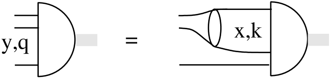
Figure 2: Diagrammatic representation of the Faddeev equation for a zero range interaction, eq. (14). The two-body input is given in Fig. 1 and eq. (1).

We now turn to the three-particle case. The expression for the two-body mass embedded in the three-body system is

$$M_{2}^{2} = (P_{3}-q)^{2}$$ (12)

$$= (M_{3}-q^{+})\left(M_{3}-\frac{\vec{q}_{\perp}^{~{}2}+m^{2}}{q^{+}}\right)-\vec{q}_{\perp}^{~{}2},$$

where $q$ denotes the momentum of the third particle. The three-body system is taken at rest, $P^{\mu}_{3}=(M_{3},0,0,0)$. In the three-body rest frame we define $x=k^{+}/M_{3}$ and $y=q^{+}/M_{3}$. Again we formally introduce an invariant regularization,

$$M^{2}_{30}<\Lambda^{2}.$$ (13)

Hence the relativistic equation (see Fig. 2) on the light front is given by

$$\Gamma_{\Lambda}(y,\vec{q}_{\perp}) = \frac{i}{(2\pi)^{3}}\ t_{\Lambda}(M_{2})\int_{0}^{1-y}\frac{dx}{x(1-y-x)}$$ (14)

$$\int d^{2}k_{\perp}\frac{\theta(M^{2}_{30}-\Lambda^{2})}{M^{2}_{3}-M_{03}^{2}}\;\Gamma_{\Lambda}(x,\vec{k}_{\perp}),$$

where we have introduced the vertex function $\Gamma_{\Lambda}$. The mass of the virtual three-particle state (in the rest system) is

$$M_{30}^{2}=\frac{\vec{k}^{~{}2}_{\perp}+m^{2}}{x}+\frac{\vec{q}^{~{}2}_{\perp}+m^{2}}{y}+\frac{(\vec{k}+\vec{q})^{2}_{\perp}+m^{2}}{1-x-y},$$ (15)

which is the sum of the on-shell minus-components of the three particles.

Equation (14) coincides with the one given previously [10] except for the regularization scheme, which we call scheme A in the following. In [10] the integration limits have been introduced to satisfy $M_{2}^{2}>0$ and hence

$$\int_{0}^{1-y}dx\int d^{2}k_{\perp}\rightarrow\int_{M^{2}/M_{3}^{2}}^{1-y}dx\int^{k_{\perp}^{\mathrm{max}}}d^{2}k_{\perp}$$ (16)

with $k_{\perp}^{\mathrm{max}}=\sqrt{(1-x)(xM_{3}^{2}-m^{2})}$. As noted correctly by  [3] in this case one no longer deals with zero range forces. In combination with (4) the invariant cut-off chosen here allows us to perform the zero range limit for $\Lambda\rightarrow\infty$. However, beyond that, the cut-off allows us to treat three-body states without two-body bound states as well, i.e. where (4) does not hold.

3 Results

We present our results in two subsections. First we focus on the more general aspects of the calculation without fixing any of the parameters. Later on we choose the parameters to reproduce the physical proton mass (as in Ref. [11]) to discuss more quantitative aspects of the approach.

Figure 3: Solution of the two- (dashed) and three-body (solid) bound state equations as a function of the strength $\lambda_{\Lambda}$ for different cut-off parameters $\Lambda=4m,6m,8m$ and $\Lambda=10^{15}m$ Figs. a,b,c, and d respectively. Horizontal dashed lines show the two-body break-up.

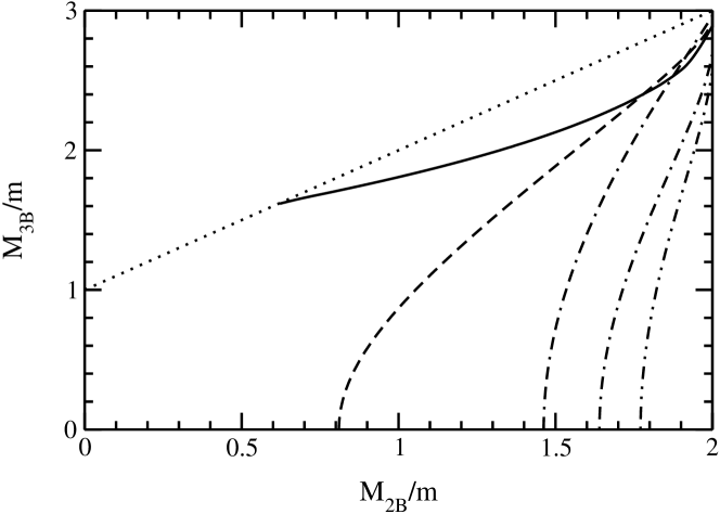
Figure 4: Three-body bound state as a function of $M_{2B}$ for different regularization schemes. Scheme A solid line. Others use invariant cut-off with different $\Lambda$: $\Lambda=4m$ (dash), $\Lambda=6m$ (dash-dot) $\Lambda=8m$ (dash-dot-dot) $\Lambda\rightarrow\infty$ (dash-dash-dot).

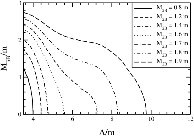
Figure 5: Three-body bound state as a function of regularization masses $\Lambda$ for different $M_{2B}$. Binding energies $M_{2B}=0.8,1.2,1.4,1.6,1.7,1.8,1.9m$ (lines left to right)

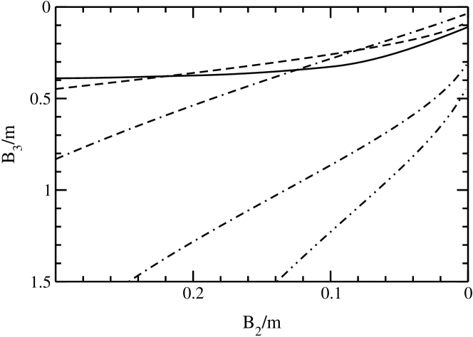
Figure 6: Binding energies $B_{3}(B_{2})$. Line coding as in Fig. 4.

3.1 General Discussion

For the more general discussion we present our results as a function of the interaction strength $\lambda$. To solve (14) we use the cut-off parameters $\Lambda=4m,6m,8m,$ where $m$ is the constituent mass, and $\Lambda/m=10^{15}\rightarrow\infty$. In Fig. 3 we show $M_{2B}$ and $M_{3B}$ (in units of m) of the solution of the two-body bound state and the three-body bound state as a function of the strength $\lambda$. Several features can be recognized:

i) The values of the strength parameter $\lambda,$ where bound states exist, become smaller as the cut-off $\Lambda$ becomes larger. This can been seen clearly, if one assumes a two-body bound state $M_{2B}$ to exist, see (4): As $\Lambda\rightarrow\infty$ and therefore $B_{2}(M_{2B})\rightarrow\infty$ the strength $\lambda\rightarrow 0$, provided the mass of the bound state is independent of the cut-off. In turn, this implies that the interaction strength depends on the cut-off, $\lambda\rightarrow\lambda_{\Lambda}$.

ii) For a certain $\lambda_{\Lambda}$ the three-body bound state shows $M_{3B}\rightarrow 0$ despite a finite value of $M_{2B}$. This is the relativistic analog of the Thomas collapse [6].

iii) As $M_{2B}\rightarrow 2m$, i.e. reaches the continuum state, the three-body bound state still exists. The parameter for which this situation occurs depends on the range of the interaction. It may give rise to the Efimov effect, an issue not further addressed here.

iv) There is a region of parameters where both $M_{2B}$ and $M_{3B}$ exist. For this particular case it is possible to plot $M_{3B}$ vs. $M_{2B}$. This has been done in previous calculations.

In fact, for case iv) we show the respective plot $M_{3B}(M_{2B})$ in Fig. 4. As explained before, using (4) as a physics input, it is possible to eliminate the $\lambda_{\Lambda}$ and $\Lambda$ dependence from the solution of the three-body equation.

A similar plot that is given in Fig. 5 shows the cut-off dependence of $M_{3B}(\Lambda)$ for a given fixed two-body mass $M_{2B}$. Again the mass $M_{3B}\rightarrow 0$ indicates the Thomas collapse.

The region close to threshold is given in Fig. 6 and parameterized in terms of the binding energies

$$B_{3} = m+M_{2B}-M_{3B}$$ (17)

$$B_{2} = 2m-M_{2B}.$$ (18)

It is worthwhile to note that for large invariant cut-off masses the resulting function $M_{3B}(M_{2B})$ coincides with the result that utilizes (4) and solves (14) without cut-off restrictions. In this sense we reproduce the result of Ref. [3]. Here we go further, extending our regularization procedure and solving the three-body equation without assuming a two-body bound state. To this end the introduction of a cut-off is adequate. On the other hand, a cut-off $\Lambda$ can be considered a physical input, e.g. as a scale limit for physics beyond the “zero range approximation” or as a range parameter of the interaction.

In Fig. 4 we have also given the earlier result using the regularization scheme A explained in the previous section. This shows no Thomas collapse, because of the additional restriction $M_{2}^{2}\geq 0$ for the intermediate state [10].

3.2 Introducing a scale

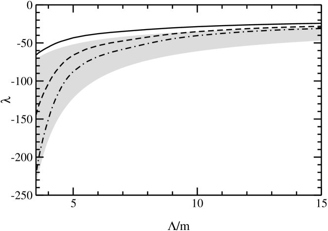
Figure 7: $\lambda(\Lambda)$ from a fit of $M_{3B}$ to the proton mass, with $m=315$ MeV (solid line), $m=400$ MeV (dashed line) $m=900$ MeV (dash-dot). Grey area bounded by $M_{2}=2m$ (upper), $M_{2}=0$ (lower).

Figure 8: Quark masses from a fit of $M_{3B}$ to the proton mass as a function of the strength $\lambda/\lambda_{0}$ for different cut-off $\Lambda$, $\lambda/\lambda_{0}=1$ as explained in the text. The dotted horizontal line indicates $m_{p}/3$. Other lines as in Fig. 4

In order to achieve more quantitative results we now introduce a scale into the calculation. Although the model is not elaborate enough to expect a complete description of the baryon dynamics we choose the proton mass $m_{p}=938$ MeV. This seems natural for a three-quark system and has been used before in this context [11]. For a more detailed description the spin has to be included on the light front, e.g., along the lines of Ref. [14]. The scale restricts the parameter space $(m,\lambda,\Lambda)$ resulting in a two-dimensional surface of allowed parameters. To be more physical we present our results in two ways. First we choose a specific quark mass (A) and second we choose a specific cut-off $\Lambda$ (B).

A. As constituent masses we choose $m\simeq m_{\rho}/2\simeq 400$MeV [11] and $m\simeq m_{p}/3\simeq 315$MeV and a rather large one of $m=900$ MeV. By fitting the proton mass this determines functions $\lambda(\Lambda)$ that are shown in Fig. 7. The grey area indicates the parameter values for which a two-body bound state exists. There are three interesting effects. i) For the weakly bound system there exists a “critical” range (parameterized through $\Lambda$) of the potential where no two-body bound state exists (lines outside the grey area). This is the case for $m=315$ MeV for all values of $\Lambda$ and for $m=400$ MeV for values of $\Lambda$ above $\sim 9.6m$. Hence there is a possibility that the nucleon could be a Borromean system. For the nonrelativistic case of Borromean systems, see e.g. [15]. ii) An intermediate quark mass already leads to the possibility of bound two-quark states. However, there is a moderate dependence on the cut-off, i.e. range of the interaction, and possibly other details of the dynamics. iii) A large quark mass ($m=900$ MeV) leads to a large “binding energy” and hence requires the existence of bound two-quark states.

B. Alternatively one may choose a particular cut-off $\Lambda$. This way, from $m_{p}=M_{3B}$ we find a relation $m(\lambda)$ that of course still depends parametrically on $\Lambda$. In Fig. 8 we show the resulting quark mass dependence necessary to reproduce the proton mass. To compare different cut-offs we have normalized the strength to the threshold strength $\lambda_{0}$, i.e. were ($M_{3B}=3m$). The dotted horizontal line indicates the continuum limit $m=m_{p}/3$.

Finally, one may wish to also fix the last parameter, $\Lambda$. To this end one could use more empirical information. This has been done in [11] for the regularization scheme A. We do not pursue this further. A detailed study of the nucleon dynamics is beyond our present aim and the capability of the model in its present form.

4 Conclusion

We have investigated in detail the stability of a relativistic three boson system subject to an effective zero range interaction. We find the relativistic analog of the Thomas collapse, which is given by $M_{3B}\rightarrow 0$. Hence, the Thomas collapse is present also for the relativistiv case, but depends on the regularization scheme. This could be seen by introducing an invariant cut-off $\Lambda$ that restricts the virtual masses in the respective few-body equations. The invariant cut-off can be understood as the limiting scale for physics beyond “zero-range approximation” or as an effective size parameter. Therefore a finite value for $\Lambda$ is meaningful. In the limit $\Lambda\rightarrow\infty$ we reproduce results given earlier [3]. For a more quantitative discussion we have introduced the nucleon mass as a scale [11]. Further analysis including a treatment of spins [14] is left for future investigations.

Acknowledgement: Work supported by Deutsche Forschungsgemeinschaft.

References

- [1] D. V. Fedorov and A. S. Jensen, hypertriton,” Nucl. Phys. A 697 (2002) 783.
- [2] D. V. Fedorov and A. S. Jensen, potentials,” Phys. Rev. A 63 (2001) 063608.
- [3] J. Carbonell and V. A. Karmanov, arXiv:nucl-th/0207073.
- [4] P. F. Bedaque and U. van Kolck, submitted to Ann. Rev. Nucl. Part. Sci., arXiv:nucl-th/0203055, and refs therein.
- [5] H. P. Noyes, Equations,” Phys. Rev. C 26 (1982) 1858.
- [6] L.H. Thomas, Phys. Rev. 47 (1935) 903.
- [7] S. K. Adhikari, T. Frederico and I. D. Goldman, Phys. Rev. Lett. 74 (1995) 487.
- [8] T. Frederico, L. Tomio, A. Delfino, A.E.A. Amorin, Phys. Rev. A 60 (1999) R9.
- [9] J. V. Lindesay and H. P. Noyes, Equations And The Efimov Effect,” SLAC-PUB-2932.
- [10] T. Frederico, Phys. Lett. B 282 (1992) 409.
- [11] W. R. de Araujo, J. P. de Melo and T. Frederico, Phys. Rev. C 52 (1995) 2733.
- [12] M. Beyer, S. Mattiello, T. Frederico and H. J. Weber, Phys. Lett. B 521 (2001) 33
- [13] S. Mattiello, M. Beyer, T. Frederico and H. J. Weber, Few Body Syst. 31 (2002) 159
- [14] M. Beyer, C. Kuhrts and H. J. Weber, Annals Phys. 269 (1998) 129
- [15] S. Moszkowski, S. Fleck, A. Krikeb, L. Theussl, J. M. Richard and K. Varga, Phys. Rev. A 62 (2000) 032504