Pair Fluctuations in Ultra-small Fermi Systems within Self-Consistent RPA at Finite Temperature

Abstract

A self-consistent version of the Thermal Random Phase Approximation (TSCRPA) is developed within the Matsubara Green’s Function (GF) formalism. The TSCRPA is applied to the many level pairing model. The normal phase of the system is considered. The TSCRPA results are compared with the exact ones calculated for the Grand Canonical Ensemble. Advantages of the TSCRPA over the Thermal Mean Field Approximation (TMFA) and the standard Thermal Random Phase Approximation (TRPA) are demonstrated. Results for correlation functions, excitation energies, single particle level densities, etc., as a function of temperature are presented.

I Introduction

Pairing properties of finite Fermi systems such as ultrasmall metallic grains have recently received a great deal of attention. This has been spurred by a series of spectacular experiments of Ralph, Black and Tinkham [1]. In order to correctly describe pairing properties it has been recognized that the finiteness of the systems (grains) needs to consider quantum fluctuations, good particle number, number parity, etc. seriously, since the coherence length may be of the order of the system size. The situation for metallic grains has in the meanwhile been well described in several review articles [2, 3] (see also [4]). Another system where the finiteness is at the forefront of the theoretical investigation since several decades is the superfluid atomic nucleus. As a matter of fact many of the theoretical tools such as particle number projection, even-odd effects, number parity, blocking effect, particle - particle Random Phase Approximation (pp-RPA), etc. have first been developed in nuclear physics [5] before finding their application to finite systems of condensed matter. Also the schematic pairing model with which we will mostly deal in this paper, namely the Picket Fence Model (PFM), whose exact solution has been found by Richardson and Sherman [6], has essentially been developed in the context of nuclear physics for the description of deformed superfluid nuclei. For finite condensed matter systems an early theoretical description was proposed by Mühlschlegel, Scalapino, and Denton [7] using the Static Path Approximation (SPA) to the partition function. This work stayed rather singular for a long time but the SPA has recently been applied successfully to the PFM both in the condensed matter [8] and nuclear [9, 10] contexts. A further standard method to treat quantum fluctuations namely the well known RPA has quite extensively been used for nuclear systems [5, 11] but equally for condensed matter problems [12].

In this work we will further elaborate on the RPA approach. We indeed have recently had quite remarkable success with a self consistent extension of the pp-RPA, which we called Self-Consistent RPA (SCRPA), by reproducing very accurately groundstate and excitation energies of the PFM [13] at zero temperature. This formalism was also developed independently by Röpke and collaborators who called it Cluster - Hartree - Fock (CHF) [14]. Such type of generalization of the RPA theory grew out of the works of K.-J. Hara and D. Rowe [15] several decades ago. Shortly afterwards the theory was rederived using the method of many body Green functions [16]. The success of the theory motivates us to develop the SCRPA formalism also for the finite temperature case and to study the thermodynamic properties of the BCS Hamiltonian using the PFM as an example. For the extension of SCRPA to finite temperature we use the Matsubara Green functions approach [17]. It appeared that the approximation scheme is very effective in treating two-body correlations in the particle-particle (pp) channel as well as the Pauli principle effects. We should mention that we will work with real particles and not with quasiparticles what should limit our approach to temperatures above the critical temperature $T_{c}$ (i.e. to the normal phase). However, as we will see below, the definition of $T_{c}$ in SCRPA is not so clear and we will be able to continue our calculation quite deeply into the superfluid regime.

We organize the paper in the following way. In Section 2, the approach is outlined in general. Then, in Section 3, the formalism is applied to the PFM. A comparison with the exact solutions as well as with the results of other approximations is made in Section 4. Section 5 is devoted to comparison with other recent works. In section 6, we will summarize the results and draw some conclusions. In an appendix a variant for the calculation of the occupation numbers is proposed.

II General formalism

In treating a finite many-body system at finite temperature, it is convenient to use the grand canonical ensemble although it violates the number conservation. With the definition

$\displaystyle K=H-\mu N$

the grand partition function and statistical operator read

$\displaystyle Z_{G}=e^{-\beta\Omega}=Tr(e^{-\beta K})$

$\displaystyle\rho_{{}_{G}}=Z_{G}^{-1}e^{-\beta K}=e^{\beta(\Omega-K)}$

where $\beta=1/T.$ Then for any Schrödinger operator $A_{\alpha}$ the modified Heisenberg picture can be introduced

$\displaystyle A_{\alpha}(\tau)=e^{K\tau}A_{\alpha}e^{-K\tau}$

and the temperature (or the Matsubara) Green’s Function (GF) is defined as [17]

$\displaystyle G_{\alpha\beta}^{\tau-\tau^{\prime}}=-\left\langle T_{\tau}A_{\alpha}(\tau)A_{\beta}^{+}(\tau^{\prime})\right\rangle=-Tr\left[e^{-\beta(K-\Omega)}T_{\tau}e^{\tau K}A_{\alpha}e^{-(\tau-\tau^{\prime})K}A_{\beta}^{+}e^{-\tau^{\prime}K}\right]=$

$$=-Tr\left[\rho_{{}_{G}}T_{\tau}e^{\tau K}A_{\alpha}e^{-(\tau-\tau^{\prime})K}A_{\beta}^{+}e^{-\tau^{\prime}K}\right]$$

Here, the brackets $\langle\phantom{O}\rangle$ mean the thermodynamic average; $T_{\tau}$ is a $\tau$ ordering operator, which arranges operators with the earliest $\tau$ (the closest to $-\beta$) to the right.

Let us consider the two-body Hamiltonian

$$H=\sum_{12}t_{12}a_{1}^{+}a_{2}+\frac{1}{4}\sum_{1234}\overline{v}_{1234}a_{1}^{+}a_{2}^{+}a_{3}a_{4}$$

where $a,\ a^{+}$ are fermion annihilation and creation operators; $t_{12}$ and $\overline{v}_{1234}=v_{1234}-v_{1243}$ are the kinetic energy and the antisymmetrized matrix element of the two-body interaction. The Green’s function $G_{\alpha\beta}^{\tau-\tau^{\prime}}$ for an arbitrary operator $A_{\alpha}^{+}$ obeys the following equation of motion:

$\displaystyle-\frac{\partial}{\partial\tau}G_{\alpha\beta}^{\tau-\tau^{\prime}}=\delta_{\tau-\tau^{\prime}}\left\langle\left[A_{\alpha},A_{\beta}^{+}\right]\right\rangle-\left\langle T_{\tau}\left[A_{\alpha},K\right]^{\tau}A_{\beta}^{+}(\tau^{\prime})\right\rangle=$

$\displaystyle=\delta_{\tau-\tau^{\prime}}N_{\alpha\beta}+\sum_{\gamma}\int d\tau_{1}^{\prime}{\cal H}_{\alpha\gamma}^{\tau-\tau_{1}^{\prime}}G_{\gamma\beta}^{\tau_{1}^{\prime}-\tau^{\prime}}$

In this expression it is possible to split the effective Hamiltonian ${\cal H}_{\alpha\beta}^{\tau-\tau^{\prime}}$ into an instantaneous and a dynamic (frequency dependent) part [18]

$${\cal H}_{\alpha\beta}^{\tau-\tau^{\prime}} = \sum_{\beta^{\prime}}\left\{\delta_{\tau-\tau^{\prime}}\left\langle\left[\left[A_{\alpha},K\right],A_{\beta^{\prime}}^{+}\right]\right\rangle-\left\langle T_{\tau}\left[A_{\alpha},K\right]^{\tau}\left[K,A_{\beta^{\prime}}^{+}\right]^{\tau^{\prime}}\right\rangle_{irr}\right\}N_{\beta^{\prime}\beta}^{-1}=$$

$$= {\cal H}_{\alpha\beta}^{(0)}\delta_{\tau-\tau^{\prime}}+{\cal H}_{\alpha\beta}^{(r)\tau-\tau^{\prime}}$$

In the approximation of the instantaneous effective Hamiltonian i.e. neglecting ${\cal H}_{\alpha\beta}^{(r)\tau-\tau^{\prime}}$, the Dyson equation for the two-body Matsubara GF $G_{\alpha\beta}^{\tau-\tau^{\prime}}$ can be written as

$$-\frac{\partial}{\partial\tau}G_{\alpha\beta}^{(0)\tau-\tau^{\prime}}=\delta_{\tau-\tau^{\prime}}N_{\alpha\beta}+\sum_{\gamma}{\cal H}_{\alpha\gamma}^{(0)}G_{\gamma\beta}^{(0)\tau-\tau^{\prime}}$$

In the treatment of two particle correlations let us specify the arbitrary operator $A_{\alpha}$ as $A_{k_{1}k_{2}}=a_{k_{1}}a_{k_{2}}$. In this case the Dyson equation (3) takes the following form in the frequency representation

$$i\omega_{n}G_{k_{1}k_{2}k_{1}^{\prime}k_{2}^{\prime}}^{SCRPA}=N_{k_{1}k_{2}k_{1}^{\prime}k_{2}^{\prime}}+\sum_{p_{1}p_{2}}{\cal H}_{k_{1}k_{2}p_{1}p_{2}}^{(0)}G_{p_{1}p_{2}k_{1}^{\prime}k_{2}^{\prime}}^{SCRPA}\,,$$

where, in supposing that the single particle density matrix is diagonal in the basis used (this is for example the case inhomogeneous matter):

$$N_{k_{1}k_{2}k_{1}^{\prime}k_{2}^{\prime}}=\left\langle\left[a_{k_{1}}a_{k_{2}},a_{k_{2^{\prime}}}^{+}a_{k_{1^{\prime}}}^{+}\right]\right\rangle=\delta_{k_{1}k_{2}k_{1}^{\prime}k_{2}^{\prime}}\left(1-n_{k_{2^{\prime}}}-n_{k_{1^{\prime}}}\right)$$

and

$${\cal H}_{k_{1}k_{2}k_{1}^{\prime}k_{2}^{\prime}}^{(0)}=\sum_{p_{1}p_{2}}\left\langle\left[\left[a_{k_{1}}a_{k_{2}},K\right],a_{p_{2}}^{+}a_{p_{1}}^{+}\right]\right\rangle N_{p_{1}p_{2}k_{1}^{\prime}k_{2}^{\prime}}^{-1}$$

Here $\delta_{k_{1}k_{2}k_{1}^{\prime}k_{2}^{\prime}}$ is the antisymmetrized Kronecker symbol and $n_{k}=\left\langle a_{k}^{+}a_{k}\right\rangle$ are the single particle occupation numbers which can be found from the single-particle Matsubara GF

$\displaystyle G_{kk^{\prime}}^{\tau}=\langle T_{\tau}a_{k}(\tau)a_{k^{\prime}}^{+}(0)\rangle$

as

$$n_{k}=\langle a_{k}^{+}a_{k}\rangle=\lim\limits_{\tau\rightarrow 0^{-}}G_{k}^{\tau}$$

In general the single-particle Matsubara Green’s function $G_{k}^{\tau-\tau^{\prime}}$ obeys the following Dyson equation:

$$\left(-\frac{\partial}{\partial\tau}+\varepsilon_{k}\right)G_{kk^{\prime}}^{\tau}=\delta(\tau)+\int d\tau_{1}M_{k}^{\tau-\tau_{1}}G_{k}^{\tau_{1}}$$

or in the frequency representation

$$G_{k}^{\omega_{n}}=G_{k}^{0}+G_{k}^{0}M_{k}G_{k}^{\omega_{n}}$$

where

$$G_{k}^{0}=\frac{1}{i\omega_{n}-\varepsilon_{k}}$$

Here $\varepsilon_{k}$ contains already the usual (instantaneous) mean field so that $M_{k}$ denotes only the dynamical part of the mass operator.

Now the problem is to find an approximation for the mass operator $M_{k}$ consistent with the SCRPA. A solution to this problem has been proposed in [18], which goes via the two body $T$ – matrix representation of the single particle mass operator [19], evaluating $T$ within SCRPA.

Let us add at this point a word of physical interpretation of the mean-field operator (6) [13]. A quick look allows to realize that it contains no higher than two body correlation functions and therefore for their determination, with (4), one obtains a selfconsistency problem. Furthermore one can consider the nucleus as a gas of zero point pair fluctuations. These fluctuations create their own mean field, i.e. one pair fluctuation moves in the average potential created by all the other pair fluctuations. This average pair fluctuation field is graphically represented in Fig. 1. It gives rise, as usual, to a nonlinear problem. Of course, the single particle mean field introduced in (9) and further developed below is coupled to the selfconsistent pair potential. This is the deeper meaning of ${\cal H}^{(0)}$ of (6).

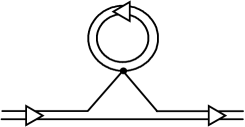
FIG. 1.: Schematic representation of the first order self-energy of a pair fluctuation. Exchange terms are not presented. The full black dot is the interaction.

III Application to the Picket Fence Model

The model consists of an equidistant multilevel pairing Hamiltonian with each level two fold degenerate, i.e. only spin up/down fermions of one kind can occupy one level. The corresponding Hamiltonian is given by

$$H=\sum_{k=1}^{\Omega}e_{k}N_{k}-G\sum_{i,k=1}^{\Omega}P_{i}^{+}P_{k}$$

with

$$N_{k}=c_{k}^{+}c_{k}+c_{\overline{k}}^{+}c_{\overline{k}},$$

$$P_{k}^{+}=c_{k}^{+}c_{\overline{k}}^{+}$$

where $\overline{k}$ means the time reversed of $k$, single particle energies are $e_{k}=k\varepsilon-\lambda,$ with level spacing $\varepsilon$ chosen to be equal to $1$, and $\Omega$ stands for the number of levels. The chemical potential $\lambda$ will be chosen such as to conserve the average number of particles $N=\Omega$ of the system. The operators defined in (12) form an SU(2) algebra for each level $j$ and obey the following commutation relations

$$\left[P_{j},P_{k}^{+}\right]=\delta_{jk}(1-N_{j}),$$

$$\left[P_{j},N_{k}\right]=2\delta_{jk}P_{j},$$

A SCRPA equations

To study the model at finite temperature we define in analogy to (1) the following set of two-body Matsubara GFs

$\displaystyle G_{ji}^{\tau}=-\left\langle T_{\tau}\overline{P}_{j}(\tau)\overline{P}_{i}^{+}(0)\right\rangle,$

where

$$\overline{P}_{j}=\frac{P_{j}}{\sqrt{<\left|1-N_{j}\right|>}}$$

Applying the instantaneous approximation for the mass operator we obtain the expressions for the two body SCRPA GF’s:

$$i\omega_{n}G_{ji}^{SCRPA}=\delta_{ji}+\sum_{k}{\cal H}_{jk}^{(0)}G_{ki}^{SCRPA},$$

with

$${\cal H}_{jk}^{(0)}=2\delta_{jk}\left(e_{j}+\frac{G}{<1-N_{j}>}\sum_{j^{\prime}}<P_{j}^{+}P_{j^{\prime}}>\right)-G\frac{<(1-N_{j})(1-N_{k})>}{\sqrt{\left|<1-N_{j}><1-N_{k}>\right|}}$$

To find the correlation functions of the form $<(1-N_{j})(1-N_{k})>$ we will use the following approximation:

when $j\neq k$ it is a simple factorization procedure, which has turned out to be accurate in the zero temperature limit:

$$<(1-N_{j})(1-N_{k})>=<1-N_{j}><1-N_{k}>$$

but when $j=k$ we use the following exact relation

$$<(1-N_{j})^{2}>=<1-N_{j}>+2<P_{j}^{+}P_{j}>$$

which can easily be obtained taking into account that $n_{j}^{2}=n_{j}$ and $n_{j}n_{\overline{j}}=P_{j}^{+}P_{j}$ (here $n_{j}=c_{j}^{+}c_{j}$). It should be noted that in [13] the factorization (16a) was also used for the diagonal part (16b) and quite accurate results were obtained. We will show below that with (16b) one obtains still improved results. As shown in [13] it is possible to avoid above approximation. However, this is at the cost of a considerable numerical complication. We refrain from this here because it brings only very little improvement of results.

With this ansatz a particle-particle RPA-like equation is obtained

$$G_{ji}^{SCRPA}=\delta_{ji}\frac{1}{z-C_{j}}-\frac{G\sqrt{\left|D_{j}D_{i}\right|}}{\left(z-C_{j}\right)\left(z-C_{i}\right)}\times\left[1+G\sum_{k}\frac{D_{k}}{z-C_{k}}\right]^{-1},$$

where

$$z=i\omega_{n},$$

$$D_{i}=<1-N_{i}>$$

and

$\displaystyle C_{j}=2\left(e_{j}-Gn_{j}+\frac{G}{D_{j}}\sum_{j^{\prime}\neq j}<P_{j}^{+}P_{j^{\prime}}>\right)$

From this one easily can find the excitation spectrum of the model in equating the denominator of (17) to zero

$$1+G\sum_{k}\frac{D_{k}}{z-C_{k}}=0$$

Knowing the poles of the Green’s function (17), one can write down its spectral representation (we here give it as a function of imaginary time), with the corresponding residua:

$\displaystyle-G_{p_{1}p_{2}}^{\tau}=\theta\left(\tau\right)\sqrt{D_{p_{1}}D_{p_{2}}}\left[X_{p_{1}}^{\mu}X_{p_{2}}^{\mu}e^{-E_{\mu}\tau}\left(1+n_{B}(E_{\mu})\right)+Y_{p_{1}}^{\mu}Y_{p_{2}}^{\mu}e^{E_{\mu}\tau}n_{B}(E_{\mu})\right]+$

$$+\theta\left(-\tau\right)\sqrt{D_{p_{1}}D_{p_{2}}}\left[X_{p_{1}}^{\mu}X_{p_{2}}^{\mu}e^{-E_{\mu}\tau}n_{B}(E_{\mu})+Y_{p_{1}}^{\mu}Y_{p_{2}}^{\mu}e^{E_{\mu}\tau}\left(1+n_{B}(E_{\mu})\right)\right]$$

$\displaystyle-G_{h_{1}h_{2}}^{\tau}=\theta\left(\tau\right)\sqrt{D_{h_{1}}D_{h_{2}}}\left[Y_{h_{1}}^{\mu}Y_{h_{2}}^{\mu}e^{-E_{\mu}\tau}\left(1+n_{B}(E_{\mu})\right)+X_{h_{1}}^{\mu}X_{h_{2}}^{\mu}e^{E_{\mu}\tau}n_{B}(E_{\mu})\right]+$

$$+\theta\left(-\tau\right)\sqrt{D_{h_{1}}D_{h_{2}}}\left[Y_{h_{1}}^{\mu}Y_{h_{2}}^{\mu}e^{-E_{\mu}\tau}n_{B}(E_{\mu})+X_{h_{1}}^{\mu}X_{h_{2}}^{\mu}e^{E_{\mu}\tau}\left(1+n_{B}(E_{\mu})\right)\right]$$

$\displaystyle-G_{ph}^{\tau}=-G_{hp}^{\tau}=\theta\left(\tau\right)\sqrt{\left|D_{p}D_{h}\right|}\left[X_{p}^{\mu}Y_{h}^{\mu}e^{-E_{\mu}\tau}\left(1+n_{B}(E_{\mu})\right)+Y_{p}^{\mu}X_{h}^{\mu}e^{E_{\mu}\tau}n_{B}(E_{\mu})\right]+$

$$+\theta\left(-\tau\right)\sqrt{\left|D_{p}D_{h}\right|}\left[X_{p}^{\mu}Y_{h}^{\mu}e^{-E_{\mu}\tau}n_{B}(E_{\mu})+Y_{p}^{\mu}X_{h}^{\mu}e^{E_{\mu}\tau}\left(1+n_{B}(E_{\mu})\right)\right]$$

$\displaystyle n_{B}\left(E_{\mu}\right)=\frac{1}{e^{\beta E_{\mu}}-1},$

where the index $p$ refers to the states above Fermi level and the index $h$ to the ones below. The following amplitudes were introduced in these formulas:

$$X_{p}^{\mu}=\frac{\sqrt{GD_{p}}}{\left|C_{p}\right|-E_{\mu}}F_{\mu},\,\,Y_{h}^{\mu}=\frac{\sqrt{-GD_{h}}}{\left|C_{h}\right|+E_{\mu}}F_{\mu}$$

$$X_{h}^{\mu}=\frac{\sqrt{-GD_{h}}}{\left|C_{h}\right|-E_{\mu}}F_{\mu},\,\,Y_{p}^{\mu}=\frac{\sqrt{GD_{p}}}{\left|C_{p}\right|+E_{\mu}}F_{\mu}$$

with

$$F_{\mu}^{-2}=\frac{\partial}{\partial z}\left[1+G\sum_{k}\frac{D_{k}}{z-C_{k}}\right]_{z=E_{\mu}}$$

These amplitudes obey the usual normalization conditions

$$\sum_{p}{}X_{p}^{\mu}X_{p}^{\mu^{\prime}}+\sum_{h}{}Y_{h}^{\mu}Y_{h}^{\mu^{\prime}}=\delta_{\mu\mu^{\prime}}$$

$$\sum_{h}{}X_{h}^{\mu}X_{h}^{\mu^{\prime}}+\sum_{p}{}Y_{p}^{\mu}Y_{p}^{\mu^{\prime}}=-\delta_{\mu\mu^{\prime}}$$

Two-body correlation functions can be obtained from the Green’s function (19) as follows

$\displaystyle<P_{p_{1}}^{+}P_{p_{2}}>=-G_{p_{1}p_{2}}^{\tau\rightarrow 0^{-}}=\sqrt{D_{p_{1}}D_{p_{2}}}\left(\sum_{\mu}X_{p_{1}}^{\mu}X_{p_{2}}^{\mu}n_{B}(E_{\mu})+\sum_{\mu}Y_{p_{1}}^{\mu}Y_{p_{2}}^{\mu}\left(1+n_{B}(E_{\mu})\right)\right)$

$$<P_{h_{1}}^{+}P_{h_{2}}>=-G_{h_{1}h_{2}}^{\tau\rightarrow 0^{-}}=\sqrt{D_{h_{1}}D_{h_{2}}}\left(\sum_{\mu}Y_{h_{1}}^{\mu}Y_{h_{2}}^{\mu}n_{B}(E_{\mu})+\sum_{\mu}X_{h_{1}}^{\mu}X_{h_{2}}^{\mu}\left(1+n_{B}(E_{\mu})\right)\right)$$

$\displaystyle<P_{p}^{+}P_{h}>=-G_{ph}^{\tau\rightarrow 0^{-}}=\sqrt{\left|D_{p}D_{h}\right|}\left(\sum_{\mu}X_{p}^{\mu}Y_{h}^{\mu}n_{B}(E_{\mu})+\sum_{\mu}Y_{p}^{\mu}X_{h}^{\mu}\left(1+n_{B}(E_{\mu})\right)\right)$

B Occupation numbers in the SCRPA

In order to close the set of the SCRPA equations, it is necessary to find the so far unknown occupation numbers $n_{k}=<c_{k}^{+}c_{k}>$ . For this, we should find the single particle Green’s function $G_{k}^{\tau}$ consistent with the SCRPA scheme. As discussed in sect. II, the single particle mass operator $M_{k}$ has in general the exact representation in terms of the two body $T$-matrix [19] and then an appropriate approximation for the $G_{k}^{\tau}$ can be obtained. It consists in using the mass operator $\widetilde{M_{k}}$ calculated through the $T$-matrix found in the framework of SCRPA. As the relation between the $T$-matrix and the sum of the all irreducible Feynman graphs in the pp-chanel is also known then the following expression for the single particle mass operator can be obtained [18]:

$$\widetilde{M_{k}}=G\sum_{k_{1}k_{2}}G_{\overline{k}}^{0(\tau_{1}^{\prime}-\tau_{1})}G_{k_{1}k_{2}}^{(\tau_{1}^{\prime}-\tau_{1})}\widetilde{{\cal H}}_{k_{2}k}^{(0)}$$

$\widetilde{\cal H}_{k_{2}k}^{(0)}$ is expressed through the effective Hamiltonian (15) without the disconnected part

$$\widetilde{\cal H}_{kk\prime}^{(0)}={\cal H}_{kk\prime}^{(0)}-2\delta_{kk\prime}\varepsilon_{k}$$

where $\varepsilon_{k}$ is defined below in (30).

In addition to this transparent scheme there also exists an additional consistency requirement [20]. It follows from the possibility to calculate the average value of the Hamiltonian $<H>$ in two ways. On the one hand one has the following relation between the single particle Green’s function (9) and $<H>$ [17]:

$$<H>=-\frac{1}{2}\lim_{\tau^{\prime}-\tau\rightarrow 0^{+}}\sum_{k}\left[\frac{\partial}{\partial\tau}-e_{k}\right]\left(G_{k}^{(\tau-\tau^{\prime})}+G_{\overline{k}}^{(\tau-\tau^{\prime})}\right)$$

On the other hand there exists the straightforward calculation of $<H>$ through the two body Green’s functions (22)

$$<H>=\sum_{k}e_{k}<N_{k}>-G\sum_{k_{1}k_{2}}<P^{+}_{k_{1}}P_{k_{2}}>$$

$$=-\frac{N^{2}}{4}+2\sum_{p}e_{p}<N_{p}>-2\sum_{p}\sum_{\mu}\sqrt{GD_{p}}F_{\mu}\left(n_{B}(E_{\mu})X_{p}^{\mu}+(1+n_{B}(E_{\mu}))Y_{p}^{\mu}\right)$$

where we used the particle-hole symmetry of the model [11] and reduced sums over p and h only to the one over the particle states.

The additional consistency condition lies in the requirement that both expressions (25) and (26) should give exactly the same results. This only is satisfied if the single particle GF is expanded to first order in the renormalized single particle mass operator (23) (one may verify that this is in analogy to the standard RPA scheme, i.e. the standard RPA average energy is obtained via (25) using a single particle GF with only perturbative renormalization from the RPA-modes):

$$G_{p}=G_{p}^{0}+G_{p}^{0}M^{SCRPA}_{p}G_{p}^{0}$$

with

$$M^{SCRPA}_{p}=\frac{\sqrt{D_{p}}}{D_{p}^{0}}\widetilde{M_{p}},$$

$$D_{p}^{0}=1-f_{p}-f_{\overline{p}}$$

$$f_{p}=\frac{1}{1+e^{\varepsilon_{p}\beta}},$$

and

$$\varepsilon_{p}=e_{p}-Gf_{p}\frac{f_{p}}{n_{p}}\frac{D_{p}}{D_{p}^{0}}.$$

Finally we get the following expression for the SCRPA single particle mass operator $M^{SCRPA}_{p}$:

$$M_{p}^{SCRPA}=\frac{\sqrt{GD_{p}}}{D_{p}^{0}}\sum_{\mu}F_{\mu}\left[\frac{S^{(1)}_{\mu p}(f_{p}+n_{B}(E_{\mu}))}{i\omega_{n}+\varepsilon_{p}-E_{\mu}}+\frac{S^{(2)}_{\mu p}(1-f_{p}+n_{B}(E_{\mu}))}{i\omega_{n}+\varepsilon_{p}+E_{\mu}}\right]\$$

where

$$S^{(1)}_{\mu p}=-\sum_{p^{\prime}}X_{p^{\prime}}^{\mu}\widetilde{\cal H}_{pp^{\prime}}+\sum_{h^{\prime}}Y_{h^{\prime}}^{\mu}\widetilde{\cal H}_{ph^{\prime}},$$

$$S^{(2)}_{\mu p}=-\sum_{p^{\prime}}Y_{p^{\prime}}^{\mu}\widetilde{\cal H}_{pp^{\prime}}+\sum_{h^{\prime}}X_{h^{\prime}}^{\mu}\widetilde{\cal H}_{ph^{\prime}}$$

The corresponding single particle occupation numbers $n_{p}$, found from (7), is the following

$$n_{p}=<c_{p}^{+}c_{p}>=f_{p}+\frac{\sqrt{GD_{p}}}{D_{p}^{0}}\sum_{\mu}F_{\mu}\left[X_{p}^{\mu}\frac{n_{B}(E_{\mu})D_{p}^{0}-f_{p}^{2}}{\left(2\varepsilon_{p}-E_{\mu}\right)}+Y_{p}^{\mu}\frac{(n_{B}(E_{\mu})+1)D_{p}^{0}+f_{p}^{2}}{\left(2\varepsilon_{p}+E_{\mu}\right)}\right]$$

$$-f_{p}\left(1-f_{p}\right)\beta\frac{\sqrt{GD_{p}}}{D_{p}^{0}}\sum_{\mu}F_{\mu}\left[X_{p}^{\mu}(f_{p}+n_{B}(E_{\mu})+Y_{p}^{\mu}(1-f_{p}+n_{B}(E_{\mu})\right]$$

Let us demonstrate now that using the single particle Green’s function (27) with the mass operator (31) and occupation numbers (32) in the calculation of the average energy (25) indeed leads to the equation (26). At first one finds the derivative of the single particle GF (27)

$$\frac{\partial G_{p}^{(\tau-\tau^{\prime})\rightarrow 0^{+}}}{\partial\tau}=-\varepsilon_{p}f_{p}+\frac{\sqrt{GD_{p}}}{D_{p}^{0}}\sum_{\mu}F_{\mu}\left\{(1-f_{p})\left[S_{\mu p}^{(1)}\frac{(\varepsilon_{p}-E_{\mu})n_{B}(E_{\mu})}{(2\varepsilon_{p}-E_{\mu})^{2}}+S_{\mu p}^{(2)}\frac{(\varepsilon_{p}+E_{\mu})(1+n_{B}(E_{\mu}))}{(2\varepsilon_{p}+E_{\mu})^{2}}\right]\right.$$

$$+\varepsilon_{p}f_{p}\left[S_{\mu p}^{(1)}\frac{f_{p}+n_{B}(E_{\mu})}{(2\varepsilon_{p}-E_{\mu})^{2}}+S_{\mu p}^{(2)}\frac{1-f_{p}+n_{B}(E_{\mu})}{(2\varepsilon_{p}+E_{\mu})^{2}}\right]$$

$$+\beta\varepsilon_{p}f_{p}(1-f_{p})\left[S_{\mu p}^{(1)}\frac{f_{p}+n_{B}(E_{\mu})}{2\varepsilon_{p}-E_{\mu}}+S_{\mu p}^{(2)}\frac{1-f_{p}+n_{B}(E_{\mu})}{2\varepsilon_{p}+E_{\mu}}\right]$$

$$-\left.f_{p}\left[S_{\mu p}^{(1)}\frac{f_{p}+n_{B}(E_{\mu})}{2\varepsilon_{p}-E_{\mu}}+S_{\mu p}^{(2)}\frac{1-f_{p}+n_{B}(E_{\mu})}{2\varepsilon_{p}+E_{\mu}}\right]\right\}=$$

$$=-\varepsilon_{p}n_{p}+\sum_{\mu}\frac{\sqrt{GD_{p}}F_{\mu}}{D_{p}^{0}}\left[S_{\mu p}^{(1)}\frac{n_{B}(E_{\mu})D_{p}^{0}-f_{p}^{2}}{2\varepsilon_{p}-E_{\mu}}+S_{\mu p}^{(2)}\frac{n_{B}(E_{\mu})D_{p}^{0}+f_{p}^{2}}{2\varepsilon_{p}+E_{\mu}}\right]$$

Inserting this expression in (25) we obtain

$$<H>=-\frac{1}{2}\lim_{\tau^{\prime}-\tau\rightarrow 0^{+}}\sum_{k}\left[\frac{\partial}{\partial\tau}-e_{k}\right]\left(G_{k}^{(\tau-\tau^{\prime})}+G_{\overline{k}}^{(\tau-\tau^{\prime})}\right)=$$

$$=-\frac{N^{2}}{4}+2\sum_{p}(e_{p}+\varepsilon_{p})n_{p}-2\sum_{p\mu}\sqrt{GD_{p}}F_{\mu}\left(n_{B}(E_{\mu})X_{p}^{\mu}+(1+n_{B}(E_{\mu}))Y_{p}^{\mu}\right)+G\sum_{p}\frac{D_{p}}{D_{p}^{0}}f_{p}^{2}=$$

$$=-\frac{N^{2}}{4}+4\sum_{p}e_{p}n_{p}-2\sum_{p}\sum_{\mu}\sqrt{GD_{p}}F_{\mu}\left(n_{B}(E_{\mu})X_{p}^{\mu}+(1+n_{B}(E_{\mu}))Y_{p}^{\mu}\right)$$

This is exactly equal to (26).

The system of the SCRPA equations is fully closed now. Together with (17), (19) and (22) this represents a self-consistent problem for pair fluctuations.

We want to indicate at this point that the above way to determine the single particle occupancies is not the only possibility. In the Appendix we will give another variant which, however, yields results close to the ones with the method of this section. The non uniqueness of the occupation numbers reflects the fact that with the truncated ansatz (3), at zero temperature, no corresponding ground state wave function can be found, as explained in [13]. For a wave function to exist, the ansatz (3) must be extended. It can, however, be shown that the correction terms are small [21].

C Exact statistical treatment of the PFM

For an exact statistical treatment of the Picket Fence Model we have to find all exact eigenvalues and eigenstates of the Hamiltonian (11). Since singly-occupied levels do not participate in the pair scattering, eigenstates can be classified according to the number of unpaired particles $S$ (seniority). There are $C_{\Omega-S}^{\Omega}=\frac{\Omega!}{S!(\Omega-S)!}$ different multiplets of this type, each of dimension $C_{\frac{N-S}{2}}^{\Omega-S}$ and degeneracy $2^{S}$. If we define the following set of basis states for each multiplet:

$$|\left\{s_{i},N_{i}\right\}>$$

where $s_{i}=N_{i}=1$ for singly-occupied levels and $s_{i}=0,N_{i}=0$ or $2$ for remaining levels ($\sum_{i}s_{i}=S$), the Hamiltonian matrix will have the following diagonal and off-diagonal elements

$$\left\langle\left\{s_{i},N_{i}\right\}\left|H\right|\left\{s_{i},N_{i}\right\}\right\rangle=\sum_{k\in S}\left(e_{k}-\lambda\right)+\sum_{k\in\Omega-S}\left[\left(e_{k}-\lambda\right)-\frac{G}{4}\left(4-N_{k}\right)\right]N_{k}$$

$$\left\langle s_{j_{1}}N_{j_{1}},...,s_{j_{k}}2,...,s_{j_{i}}0,...,s_{j_{n}}N_{j_{n}}\left|H\right|s_{j_{1}}N_{j_{1}},...,s_{j_{k}}0,...,s_{j_{i}}2,...,s_{j_{n}}N_{j_{n}}\right\rangle=-G$$

The exact eigenvalues and eigenstates can be calculated by diagonalization of this matrix in each multiplet. The exact grand canonical average $<A>$ of any operator can then be obtained with the help of the grand partition function $Z_{G}=Tre^{-\beta\hat{H}}$ and the statistical operator $\hat{\rho_{G}}=Z_{G}^{-1}e^{-\beta\hat{H}}$ as

$$<A>=Tr[\hat{A}\hat{\rho_{G}}]$$

IV Results and Discussion

In order to check the accuracy of our theory and of the different approximations schemes we first calculate the average energy of the system $<H>$ as a function of the particle number $N$ and temperature $T$. The results of the different calculations are presented in Figures 2 – 4. Calculations were made for a value of the pairing constant $G$ which is smaller but close to the critical value $G_{cr}$ at $T=0$. The phase transition from the normal to the superfluid phase occurs in the system when $G\to G_{cr}$ . We compare the SCRPA results with the exact ones for the Grand Canonical Ensemble (GCE) as well as results of the standard Thermal RPA (TRPA) and Thermal MFA (TMFA). One can see that when the number of levels $\Omega$ (and number of particles $N$) increases the description of the intrinsic energy becomes better and at $\Omega=N=10$ the TSCRPA results practically coincide with the exact ones. Especially the last case will be considered below more carefully.

Let us now come to the discussion of the behavior of the excitation energies. The dependence of the excitation energies of the addition mode (see [13]) as a function of $G$ is shown in Fig. 5 at zero temperature. The SCRPA (solid lines) is compared with the standard RPA calculations (dashed lines) and the exact ones (open circles). Increasing the interaction constant, the lowest energy in the RPA goes to zero and at $G_{cr}\simeq 0.33$ the collapse takes place which is connected with the transition from the normal to the superfluid phase. At finite temperature (see Fig. 6 where the dependence of the lowest addition mode is presented as a function of $G$ at $T=0.5$) this collapse occurs at a higher value of the interaction constant ($G_{cr}\simeq 0.43$) what is due to the reduced intensity of the residual interaction because of the thermal factors. This collapse is absent in the exact calculations at zero temperature and also in the SCRPA calculations at zero and finite temperatures. It is also remarkable that the SCRPA yields a rise of all excitation energies with increasing $G$ in contrast with RPA and in very good agreement with the exact results. This comes from the fact that in the PFM with the Kramer’s degeneracy of levels the Pauli repulsion is extremely strong overruling the original attractive interaction. In this model, therefore, standard RPA gives qualitatively wrong result.

We next consider the behavior of the system near the phase transition point. To make distinctions between different results more apparent we not only show the full intrinsic energy $<H>$ but also the correlation energy $E_{corr}$ which is defined as

$$E_{corr}=<H>-<H>_{0}$$

where $<H>_{0}$ is the average energy calculated in Mean Field Approximation. In Figures 7 and 8, the average energy $<H>$ and correlation energy $E_{corr}$ as a function of $T$ are displayed for the interaction constant $G=0.4$ (at $T=0$ this value of $G$ is larger than $G_{cr}\simeq 0.33$). With increasing $T$ the mean field rearrangement occurs and the system goes from the superfluid phase to the normal one at $T_{c}\simeq 0.38$. Note, that within the TRPA the lowest excitation energy $\omega_{1}$ vanishes when $T\rightarrow T_{c}$, whereas within the TSCRPA $\omega_{1}$ stays finite. For both the correlation energy and the intrinsic energy the TSCRPA gives more precise results as compared to the other approximations. It is remarkable that the TSCRPA results are accurate down to practical zero temperature, in spite of the fact that within standard BCS theory one enters the superfluid regime. A quasiparticle formulation of SCRPA [22] will only be necessary for stronger $G$ values driving the system more deeply into the symmetry broken phase.

To analyze the region near the phase transition point in more detail, the heat capacity is calculated as a partial derivative of the intrinsic energy with respect to $T$

$$C_{v}=\frac{\partial<H>}{\partial T}$$

The results are shown in Fig. 9. The TRPA and TMFA give discontinuities of $C_{v}$ at $T_{c}$ (we recall again that our results are obtained using a normal fluid approach and not transforming to quasiparticles). The heat capacity calculated in the TSCRPA has some kink near $T_{c}$ but has no discontinuities and is quite similar to the exact result through out the whole range of temperature.

Nevertheless, the TSCRPA and also the exact solution feel the phase transition to the superfluid phase. It can be seen in Fig. 8 where both the TSCRPA and the exact correlation energies show a depression near $T=0.38$. This originates from strong pair fluctuations leading to the BCS phase transition in TMFA with the critical temperature $T_{cr}^{BCS}=0.38$ for $G=0.4$. However, one notices (see also [23]) that the sharp phase transition of mean field is in reality completely smeared out and only a faint, though clearly visible, signal survives.

To investigate the formation of such fluctuations in more detail, it is useful to consider the spectral function [17]

$$A(k,\omega)=\frac{1}{i}\left[G_{k}^{\omega_{n}}\biggl{|}_{i\omega_{n}\rightarrow\omega-i\eta}-G_{k}^{\omega_{n}}\biggr{|}_{i\omega_{n}\rightarrow\omega+i\eta}\right]$$

which includes two-body correlations through the self-consistent treatment of the mass operator $M_{k}^{SCRPA}(\omega_{n})$. Based on the spectral function the density of states can be calculated as [24]

$$N(\omega)=\sum_{k}A(k,\omega)$$

The results of the calculations of $N(\omega)$ with $G_{k}$ of (27) in (39) are shown in Fig. 10 at different values of $T$ and for $G$ = 0.4. It is clearly seen that the distance between the two quasiparticle peaks around the Fermi energy $\varepsilon_{F}$ ($\omega=0$) increases with decreasing temperature. This process sets in even above the BCS transition temperature $T_{c}^{BCS}=0.38$. This rarefaction of the level density around $\varepsilon_{F}$ above $T_{c}$ is not avoid of similarity with the situation in high $T_{c}$ – superconductors where a so-called ’pseudo gap’ in the level density appears already above $T_{c}$ [25]. This ’pseudo gap’ also is often attributed to a decrease in the level density around $\varepsilon_{F}$ due to pair fluctuations [24, 26]. Apparently it is a quite generic feature that pair correlations diminish the density of levels around $\varepsilon_{F}$ whereas particle-hole correlations give rise to an increase.

In order to make the temperature dependence of the gap more transparent let us introduce an effective (or canonical) gap which recently was proposed in Eq. (22) of Ref. [3]

$$\Delta=G\sqrt{\sum_{ik}\left(\langle P_{i}^{+}P_{k}\rangle-\left\langle c_{i}^{+}c_{k}\right\rangle\left\langle c_{\overline{i}}^{+}c_{\overline{k}}\right\rangle\right)}$$

In the BCS approximation, the effective gap $\Delta$ coincides with the usual grand canonical BCS gap

$$\Delta_{0}=G\sum_{k}\langle P_{k}\rangle_{BCS}$$

The dependencies of the effective gap on the interaction constant $G$ at zero temperature and on temperature $T$ at $G=0.4$ are shown in Figures 11 and 12. The SCRPA results give a very good description of the gap at zero and non zero temperatures. It is clearly seen that the SCRPA and exact calculations do not display the phase transition at the point where the BSC gap vanishes. Notice that in Fig. 11 the SCRPA result deteriorates for values of $G$ well beyond the critical value. In this regime a quasiparticle generalization of the SCRPA is necessary [22] because one enters deeply in the superfluid region.

V Comparison with other works

The PFM has recently widely been used for the study of quantum pair fluctuations at finite temperature both in the context of nuclear physics [9, 10] and of ultrasmall metallic grains [8, 4]. In both fields the SPA approach where one additionally takes into account number parity projection and quantum (RPA) fluctuation around mean field was employed.

To compare our results with the above mentioned formalism let us introduce the relevant energy scales. These are the average level spacing $\delta$ and the BCS energy $\Delta=\Omega\delta/[2\sinh(\delta/G)]$ [2, 3]. The properties of the system described by the pairing Hamiltonian can be calculated as universal functions of the single scaling parameter $\delta/\Delta$. As long as the grain is not too small $\delta<<\Delta$, the fluctuation region around $T_{c}$ is narrow, and the mean field (BCS) description of superconductivity is appropriate. It is the case in ref. [10], where the PFM is investigated with characteristic values of $\delta/\Delta\simeq 0.2$. The result of that work shows that the domain where the parity projection is important lies in a small region near $T_{c}$. At temperatures higher than $T_{c}$ the role of the fluctuation is decreased and usual SPA becomes rather good in reproducing the exact canonical results.

When the size of the system is decreased, fluctuations start to smear the normal – superconducting transition. The finite level spacing suppresses the BCS gap and when $\delta$ becomes of the order of $\Delta$, the fluctuation region becomes of order $T_{c}$ and the BCS description of superconductivity breaks down even at zero temperature. Returning to our calculations, we can see that SCRPA yields the best results for $\delta/\Delta\geq 1$ (see Fig. 11, 12). This region corresponds to ultrasmall grains where strong pairing fluctuations are dominant. In this sense our results can be compared (at least qualitatively) with the results of [8]. To make this comparison more accurate we calculated average energy and specific heat for a system with 50 fermions and interaction constant $G=0.127$ and $G=0.255$, what corresponds to $\delta/\Delta=50$ and $\delta/\Delta=1$ respectively. In general our results correlate well with [8]. From Fig. 13, where $C_{v}$ is displayed as a function of $T/\delta$, we can see that when $\delta/\Delta\to\infty$ the specific heat approaches a linear dependence with temperature while when $\delta\sim\Delta$ a bump structure arises at low temperature which is a sign of the presence of strong pairing fluctuations. As it has been seen from our previous discussion, the SCRPA gives a better description with increasing particles number. And while we did not perform exact GCE calculations for the system with 50 particles, we can expect from our studies above and in [13] that our result should be very close to the exact one.

In conclusion of this section we can say that the results of TSCRPA are at least as good as the ones of SPA with extensions. However, contrary to SPA, TSCRPA has no problem at low temperature and excitation energies and correlation functions can be calculated directly as a function of temperature.

VI Conclusion

In this work we generalized our recent work [13] on the multilevel pairing model (PFM) within the SCRPA approach to finite temperature (TSCRPA). The PFM has been recognised to account in many respects for the physics of (superconducting) metallic nano-grains. In our context SCRPA can be viewed as a self-consistent mean field theory for pair fluctuatuations. The results at $T=0$ in [13] are in very close agreement with the exact ones obtained from the Richardson procedure [5]. It is therefore an important issue to also exploit SCRPA at finite $T$ and to assess its accuracy with respect to exact results in this case. Our comparison is mostly done for the case of ten levels with $10$ particles where it is still of some ease to establish the exact partition function. We, however, also considered with TSCRPA the case of 50 particles in $50$ levels assuming that the results are of equal quality or even better as the ones obtained for $10$ particles. We base our studies on the Matsubara $1$ and $2$ particle Green’s functions which allows us to calculate correlation and excitation energies, specific heat, level densities, etc. It can be considered as a general advantage of our approach that all these quantities are directly accessible in the whole range of temperatures and coupling constants. For the latter this holds in this work only true for interaction values not driving the system deeply into the superfluid regime, since in this work we only have been working with normal particles and not with quasiparticles. For $G>>G_{cr}$ we have to employ the Self Consistent Quasiparticle RPA (SCQRPA). It has recently been demonstrated in the two level pairing model that also SCQRPA gives very promising results [22]. The quality of our results for the above mentioned quantities turns out to be excellent and it does not fail in any qualitative nor quantitative aspect. Most of the time the agreement with the exact solution is within the couple of percent level. One particularly interesting feature of our investigation is the fact that we achieved to calculate the single particle Green’s function consistently within TSCRPA. This enabled us to give, for the first time, for the PFM the evolution of the single particle level density with temperature. The construction of the exact solution for this quantity is very cumbersome and we refrained from working this out here. However, backed with the positive experience for all other above mentioned quantities we believe that also the level density is reasonably accurate. The interesting aspect of our calculation is that with decreasing temperature the density of single particle states around the Fermi level decreases even above the critical temperature as defined by BCS – theory. It is suggestive to see this feature in analogy to the appearance of a so called pseudogap in high $T_{c}$ superconductors where also a depression in the level density is observed approaching $T_{c}$ from above [24, 25]. It would be interesting to attempt an experimental verification with metallic nanograins of our prediction that indeed the density of levels rarefies with decreasing temperature already in the non superfluid regime.

We also gave a short comparison of TSCRPA with results at finite $T$ obtained with other approaches like the static path approximation (SPA) to the partition function. Though the results seem generally comparable, we think that TSCRPA is more versatile, giving direct access to correlation functions, level densities, excitation energies, etc. in the whole temperature range, quantities which are otherwise difficult to obtain.

In the present work we restricted ourselves to values of the coupling which are below or slightly above the critical value. In the future we shall elaborate on the SCRPA for quasiparticles at finite $T$ (TSCQRPA) which will allow us to consider the system deeply in the superfluid phase and to study the transition from one phase to the other in more detail.

ACKNOWLEDGMENTS

We acknowledge useful discussions with P. Bozek, F. Hekking and J. Hirsch.

APPENDIX: OCCUPATION NUMBER – VARIANT

Let us give another possible way to find the occupation numbers at finite temperature. Before to complete this task we firstly derive the SCRPA equations with the Equation of Motion method and find some useful relations between phonon amplitudes at zero temperature. To attain this let us introduce the pair addition and removal operators (phonons) [13] as

$$Q_{\mu}^{+}=\sum_{p}X_{p}^{\mu}\overline{P}_{p}^{+}-\sum_{h}Y_{h}^{\mu}\overline{P}_{h}^{+}$$

$$Q_{\lambda}^{+}=\sum_{h}X_{h}^{\lambda}\overline{P}_{h}-\sum_{p}Y_{p}^{\lambda}\overline{P}_{p}$$

and apply the variational procedure where all expectation values are found with respect to the vacuum of phonons (A1,A2).

$$<\left[\delta Q_{\nu},\left[{\cal H},Q_{\nu}^{+}\right]\right]>=\omega_{\nu}<\left[\delta Q_{\nu},Q_{\nu}^{+}\right]>$$

If we use the factorisation procedure (16) the following system of equations for the phonon amplitudes is obtained

$$\sum_{p^{\prime}}X_{p^{\prime}}^{\mu}A_{pp^{\prime}}-\sum_{h^{\prime}}Y_{h^{\prime}}^{\mu}B_{ph^{\prime}}=E_{\mu}X_{p}^{\mu}$$

$$\sum_{p^{\prime}}X_{p^{\prime}}^{\mu}B_{hp^{\prime}}-\sum_{h^{\prime}}Y_{h^{\prime}}^{\mu}C_{hh^{\prime}}=-E_{\mu}Y_{h}^{\mu},$$

where

$$A_{pp^{\prime}}=2\delta_{pp^{\prime}}[e_{p}]+2G\delta_{pp^{\prime}}\left[\sum_{l\neq p}\frac{<P_{l}^{+}P_{p}>}{D_{p}}-n_{p}\right]-G\sqrt{D_{p}D_{p^{\prime}}}=2\delta_{pp^{\prime}}\varepsilon_{p}+\widetilde{A}_{pp^{\prime}}$$

$$B_{ph}=-G\sqrt{-D_{p}D_{h}}$$

$$C_{hh^{\prime}}=2\delta_{hh^{\prime}}[e_{h}-G]+2G\delta_{hh^{\prime}}\left[\sum_{l\neq h}\frac{<P_{l}^{+}P_{h}>}{D_{h}}+1-n_{h}\right]-G\sqrt{D_{h}D_{h^{\prime}}}=-\left(2\delta_{hh^{\prime}}\varepsilon_{h}+\widetilde{C}_{hh^{\prime}}\right)$$

$$B_{hp}=-G\sqrt{-D_{h}D_{p}}$$

where the single-particle energies are introduced as

$$\varepsilon_{p}=e_{p},\varepsilon_{h}=-e_{h}+G$$

Thereafter the expressions for the phonon amplitudes are obtained as

$$X_{p}^{\mu}(2\varepsilon_{p}-E_{\mu})=-\sum_{p^{\prime}}X_{p^{\prime}}^{\mu}\widetilde{A}_{pp^{\prime}}+\sum_{h^{\prime}}Y_{h^{\prime}}^{\mu}B_{ph^{\prime}}\Longrightarrow X_{p}^{\mu}=\frac{-\sum_{p^{\prime}}X_{p^{\prime}}^{\mu}\widetilde{A}_{pp^{\prime}}+\sum_{h^{\prime}}Y_{h^{\prime}}^{\mu}B_{ph^{\prime}}}{2\varepsilon_{p}-E_{\mu}}$$

$$Y_{h}^{\mu}(2\varepsilon_{h}+E_{\mu})=-\sum_{p^{\prime}}X_{p^{\prime}}^{\mu}B_{hp^{\prime}}+\sum_{h^{\prime}}Y_{h^{\prime}}^{\mu}\widetilde{C}_{hh^{\prime}}\Longrightarrow Y_{h}^{\mu}=\frac{-\sum_{p^{\prime}}X_{p^{\prime}}^{\mu}B_{hp^{\prime}}+\sum_{h^{\prime}}Y_{h^{\prime}}^{\mu}\widetilde{C}_{hh^{\prime}}}{2\varepsilon_{h}+E_{\mu}}$$

Due to the particle-hole symmetry, the removal mode satisfy exactly the same equations. It means that

$$X_{p}^{\mu}=X_{h=N-p+1}^{\lambda=\mu},Y_{h}^{\mu}=Y_{p=N-h+1}^{\lambda=\mu}$$

Below we will use the notation $\mu$ for both modes.

Returning to the single particle occupation numbers $n_{k}$ let us remind that in the picket fence model the following exact relation between one body operator $N_{k}$ and two body operator $P_{k}^{+}P_{k}$ is verified for any non singly-occupied level $k$:

$$N_{k}=2P_{k}^{+}P_{k}$$

Taking the average of both parts of this relation with respect to the SCRPA vacuum state we obtain

$$<N_{p}>=2D_{p}\sum_{\mu}(Y_{p}^{\mu})^{2}$$

On the other hand, using relations (A7) we can rewrite this expression as

$$<N_{p}>=2D_{p}\sum_{\mu}\frac{1}{\left(E_{\mu}+2\epsilon_{p}\right)^{2}}\left[\sum_{h}X_{h}^{\mu}B_{ph}-\sum_{p^{\prime}}Y_{p^{\prime}}^{\mu}\widetilde{C}_{pp^{\prime}}\right]\left[\sum_{h}X_{h}^{\mu}B_{hp}-\sum_{p^{\prime}}Y_{p^{\prime}}^{\mu}\widetilde{C}_{p^{\prime}p}\right]$$

It is easy to show that the fraction in this expression can be expressed through the GFs as

$$\frac{1}{\left(E_{\mu}+2\epsilon_{p}\right)^{2}}=-\lim_{t^{\prime}-t\rightarrow 0^{+}}\int\int dt_{1}^{\prime}dt_{1}G_{p}^{0(t-t_{1})}\theta(t_{1}^{\prime}-t_{1})e^{-i(E_{\mu}+\varepsilon_{p})(t_{1}^{\prime}-t_{1})}G_{p}^{0(t_{1}^{\prime}-t^{\prime})}$$

where

$$G_{p}^{0(t-t_{1})}=-i<T_{t}c_{p}(t)c_{p}^{+}(t_{1})>=-i\theta(t-t_{1})e^{-i\varepsilon_{p}(t-t_{1})}$$

If we now take into account the spectral representation of the pair operator $P_{p}$

$$P_{p}(t)=D_{p}\left[\sum_{\mu}e^{-iE_{\mu}t}Q_{\mu}X_{p}^{\mu}+\sum_{\mu}e^{iE_{\mu}t}Q_{\mu}^{+}Y_{p}^{\mu}\right]$$

and define the antichronological (time reversed) single particle GF as

$$G_{\overline{p}}^{0(t-t_{1})}=-i<T_{t}c_{\overline{p}}^{+}(t)c_{\overline{p}}(t_{1})>=-i\theta(t_{1}-t)e^{i\varepsilon_{p}(t-t_{1})}$$

we can pass to the expression for the sp GF which gives occupation numbers which are consistent within the frame of the SCRPA with exact relation (A9)

$$G_{p}^{\left(t-t^{\prime}\right)}=G_{p}^{0(t-t^{\prime})}+\int\int dt_{1}dt_{1}^{\prime}G_{p}^{0(t-t_{1})}M^{SCRPA}_{p}G_{p}^{0(t_{1}^{\prime}-t^{\prime})}$$

where $M^{SCRPA}_{p}$ is a single particle mass operator

$$M^{SCRPA}_{p}=\sum_{k_{1}k_{2}}G_{\overline{p}}^{0(t_{1}^{\prime}-t_{1})}\overline{{\cal H}}_{pk_{1}}^{(0)}G_{k_{1}k_{2}}^{(t_{1}^{\prime}-t_{1})}\overline{{\cal H}}_{pk_{2}}^{(0)}$$

and $\overline{{\cal H}}_{pk}^{(0)}$ is the renormalised effective Hamiltonian which has the following form in terms of RPA matrixes $A_{pp^{\prime}}$ and $B_{ph}$

$$\overline{{\cal H}}_{pp^{\prime}}^{(0)}=\sqrt{D_{p}}\widetilde{A}_{pp^{\prime}}\frac{1}{\sqrt{D_{p^{\prime}}}}$$

$$\overline{{\cal H}}_{ph}^{(0)}=\sqrt{D_{p}}B_{ph}\frac{1}{\sqrt{-D_{h}}}$$

From (A16) and (A17) we then can define the occupation numbers as usual. In general, the occupation numbers from (32) and (A16), (A17) have slightly different values. This is due to the fact that the ansatz (A1), (A2) for the RPA operators is too restricted for a groundstate fulfilling $Q|0>=0$ to exist. It can, however, be shown [21] that the necessary corrections to (A1), (A2) are small. Anyhow, the differences in occupation numbers obtained from the two methods are a measure of the importance of the terms neglected in (A1), (A2). The difference of the mass operators (23) and (A17) is that in the latter both vertices are dressed, whereas in (23) one vertex remains at the unrenormalized value (G).

To find occupation numbers $<n_{p}>$ at finite temperature we adopt the expressions obtained for single particle GF at zero temperature (eq.(A16)-(A18)). To do it, it is necessary to change all zero temperature GFs to the Matsubara ones and use for the vertices the renormalised effective Hamiltonian (15)

$$\overline{{\cal H}}_{pk}^{(0)}=\sqrt{D_{p}}\widetilde{{\cal H}}_{pk}^{(0)}\frac{1}{\sqrt{\left|D_{k}\right|}}$$

where

$$\widetilde{\cal H}_{pk}^{(0)}={\cal H}_{pk}^{(0)}-2\delta_{pk}\varepsilon_{k}$$

and

$$\varepsilon_{k}=e_{k}-Gf_{k},$$

$$f_{k}=\frac{1}{1+e^{\varepsilon_{k}\beta}}$$

Then we get for the single particle Matsubara GF

$$G_{p}^{\left(\tau-\tau^{\prime}\right)}=G_{p}^{0(\tau-\tau^{\prime})}+\int\int d\tau_{1}d\tau_{1}^{\prime}G_{p}^{0(\tau-\tau_{1})}M^{SCRPA}_{p}G_{p}^{0(\tau_{1}^{\prime}-\tau^{\prime})}$$

$$=G_{p}^{0(\tau-\tau^{\prime})}+\int\int d\tau_{1}d\tau_{1}^{\prime}G_{p}^{0(\tau-\tau_{1})}\left[\sum_{k_{1}k_{2}}G_{\overline{p}}^{0(\tau_{1}^{\prime}-\tau_{1})}\overline{{\mathcal{H}}}_{pk_{1}}^{(0)}G_{k_{1}k_{2}}^{(\tau_{1}^{\prime}-\tau_{1})}\overline{{\mathcal{H}}}_{pk_{2}}^{(0)}\right]G_{p}^{0(\tau_{1}^{\prime}-\tau^{\prime})}$$

where

$$G_{p}^{0(\tau-\tau^{\prime})}=-e^{-\varepsilon_{p}(\tau-\tau^{\prime})}\left[\theta\left(\tau-\tau^{\prime}\right)(1-f_{p})-\theta\left(\tau^{\prime}-\tau\right)f_{p}\right],$$

Taking this integral in the limit $\tau-\tau^{\prime}\longrightarrow 0^{-}$ we obtain the occupation numbers $n_{p}$ in the SCRPA at finite temperature

$\displaystyle n_{p}=<c_{p}^{+}c_{p}>=f_{p}+D_{p}\sum_{\mu}\left(Y_{p}^{\mu}\right)^{2}\left[n_{B}\left(E_{\mu}\right)\left(1-2f_{p}\right)+\left(1-f_{p}\right)^{2}\right]$

$\displaystyle+D_{p}\sum_{\mu}\left(X_{p}^{\mu}\right)^{2}\left[n_{B}\left(E_{\mu}\right)\left(1-2f_{p}\right)-\left(f_{p}\right)^{2}\right]$

$\displaystyle-f_{p}\left(1-f_{p}\right)\beta D_{p}\left[\sum_{\mu}\left(Y_{p}^{\mu}\right)^{2}\left(1+n_{B}\left(E_{\mu}\right)-f_{p}\right)\left(2\varepsilon_{p}+E_{\mu}\right)\right]$

$$-f_{p}\left(1-f_{p}\right)\beta D_{p}\left[\sum_{\mu}\left(X_{p}^{\mu}\right)^{2}\left(n_{B}\left(E_{\mu}\right)+f_{p}\right)\left(2\varepsilon_{p}-E_{\mu}\right)\right]$$

One should note here one thing about the direct use of the exact relation (A9) for the definition of the $<N_{p}>$. In reality the identity (A9) is only valid for the collective subspace (spanned by the non singly-occupied levels) or, in other words, for levels which have partial seniority $s_{k}=0$. But when we work in the grand canonical ensemble, seniority of the level $s_{k}$ is not a good quantum number, since averaging procedure over GCE mixes all seniorities. This fact is reflected in the above expression (A21) where we can see that level occupation numbers $<N_{p}>=n_{p}+n_{\bar{p}}$ due to thermal factors $f_{p}$ (Fermi-Dirac distribution) are not equal to $<2P^{+}_{p}P_{p}>$.

Before coming to a numerical example let us make a further comment. Knowing the occupation numbers as a function of the amplitudes $X$ and $Y$ as in (A21) or (32), a natural idea would be to use this to express the ground state energy entirely as a function of $X$ and $Y$. Then minimizing under the constraint of the normalization conditions (21) leads to an equation determining $X,Y$ amplitudes. Such a procedure has been proposed in the past by Jolos and Rybarska [27]. However, already in our example where the occupation numbers are exactly known (at zero temperature) as a function of $X,Y$ amplitudes, we have checked that this leads to worse results than with the approach advanced in the main text. In other examples the functional $n_{p}[X,Y]$ may only be known approximately and then the minimization of the ground state leads to deteriorated results, as we also have checked. In the Green’s function approach where one first calculates excitation energies, i.e. energy differences, before calculating the ground state energy, such uncertainties like the precise knowledge of $n_{p}[X,Y]$ are minimized and the solution of the SCRPA equations is therefore much more stable.

Let us now compare the results based on the two different definitions of the occupation numbers (eq. (32) and (A21)). We will denote results with eq. (32) by TSCRPA and results obtained with the second definition (eq. (A21)) by TSCRPA1. All calculations are made for the system with 10 particles on 10 levels. Results for the correlation energy (37) as a function of the coupling constant $G$ are given in Tab. 1 and Tab. 2 for $T=0$ and $T=1$, respectively. In these tables we denote results obtained with (A21) and (26) by TSCRPA1-1 and the ones obtained with (A21) and (25) by TSCRPA1-2. We can see that TSCRPA systematically gives underestimated results with respect to the exact ones. Using definition (A21) we then can see that TSCRPA1-1 at zero temperature slightly overestimates the exact ground state energy (this corresponds to the results given in [13]) while TSCRPA1-2 always underestimates it. At finite temperature all approximations (TSCRPA and TSCRPA1) give close results which underestimate the exact ones. In Tab. 3 and 4 we show excitation energies of the first addition mode for $T=0$ and $T=1$. In both cases, TSCRPA and TSCRPA1, excitation energies grow with increasing $G$ for zero and nonzero temperatures reproducing quite well the exact results. We can see that for the calculated quantities (correlation and excitation energies) TSCRPA1-1 is slightly closer to the exact results than TSCRPA.

Table 1. Correlation energy as function of $G$ at zero temperature.

G	Exact	TSCRPA1-1	TSCRPA1-2	TSCRPA
0.10	-0.036	-0.037	-0.036	-0.036
0.20	-0.167	-0.169	-0.153	-0.159
0.30	-0.435	-0.445	-0.342	-0.379
0.33	-0.551	-0.564	-0.408	-0.461
0.34	-0.593	-0.608	-0.430	-0.489
0.35	-0.638	-0.654	-0.453	-0.518
0.36	-0.685	-0.702	-0.476	-0.548
0.40	-0.896	-0.917	-0.569	-0.670

Table 2. Correlation energy as function of $G$ at $T=1$.

G	Exact	TSCRPA1-1	TSCRPA1-2	TSCRPA
0.10	-0.030	-0.029	-0.018	-0.029
0.20	-0.142	-0.126	-0.082	-0.122
0.30	-0.372	-0.299	-0.208	-0.295
0.33	-0.476	-0.367	-0.259	-0.365
0.34	-0.515	-0.392	-0.278	-0.391
0.35	-0.556	-0.418	-0.297	-0.417
0.36	-0.600	-0.444	-0.317	-0.445
0.40	-0.803	-0.559	-0.403	-0.569

Table 3. Excitation energy of the first addition mode as function of $G$ at $T=0$.

G	Exact	TSCRPA1	TSCRPA
0.10	1.001	1.001	1.001
0.20	1.005	1.012	1.012
0.30	1.014	1.049	1.053
0.33	1.018	1.068	1.074
0.34	1.019	1.075	1.081
0.35	1.022	1.082	1.089
0.36	1.023	1.089	1.098
0.40	1.031	1.123	1.136

Table 4. Excitation energy of the first addition mode as function of $G$ at $T=1.0$.

G	TSCRPA1	TSCRPA
0.10	1.017	1.030
0.20	1.075	1.126
0.30	1.175	1.281
0.40	1.299	1.476
0.41	1.312	1.497
0.42	1.324	1.518
0.43	1.337	1.539
0.44	1.349	1.560
0.45	1.362	1.581

FIG. 2.: The average energy $<H>$ as a function of the temperature for $\Omega=N=2$ and $G=0.9$. The exact results – open circles; the TMFA results – dotted line; the TRPA results – dashed line and the TSCRPA results – solid line.

FIG. 3.: The average energy $<H>$ as a function of the temperature for $\Omega=N=4$ and $G=0.5$. For notation, see Fig.2

FIG. 4.: The average energy $<H>$ as a function of the temperature for $\Omega=N=10$ and $G=0.33$. For notation, see Fig.2.

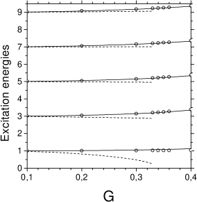
FIG. 5.: Excitation energies as a function of the interaction constant $G$ for $\Omega=10$ and $T=0$. Notations: the exact results – open circles; TRPA results – dashed lines and the TSCRPA results – solid lines.

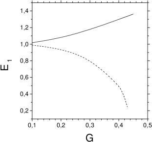
FIG. 6.: The first excitation energy $E_{1}$ as a function of the interaction constant $G$ for $\Omega=10$ and $T=0.5$. Notations: TRPA results – dashed line, the TSCRPA results – solid line.

FIG. 7.: The average energy $<H>$ as a function of the temperature for $\Omega=N=10$ and $G=0.4$. For notation, see Fig.2.

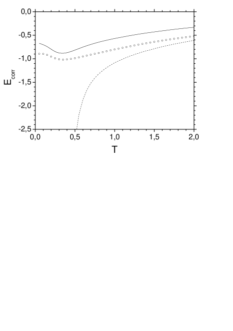
FIG. 8.: The correlation energy $E_{corr}$ as a function of the temperature for $\Omega=N=10$ and $G=0.4$. For notation, see Fig.2.

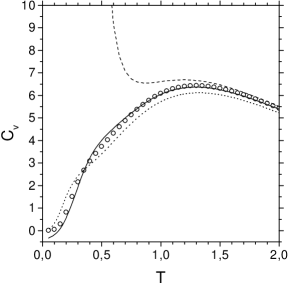
FIG. 9.: The heat capacity $C$ as a function of the temperature for $\Omega=N=10$ and $G=0.4$. For notation, see Fig.2.

FIG. 10.: The density of states as a function of the frequency $\omega$ for $\Omega=N=10$, $G=0.4$ and $T=0.05$, $T=0.25$, $T=0.45$ and $T=1.05$.

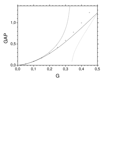
FIG. 11.: The effective gap $\Delta$ as a function of the interaction constant $G$ for $\Omega=N=10$ and $T=0$. The exact results – open circles; the BCS results – dotted line; the RPA results – dashed line and the SCRPA results – solid line.

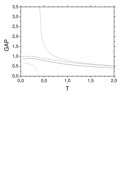
FIG. 12.: The effective gap $\Delta$ as a function of the temperature $T$ calculated for $\Omega=N=10$ and $G=0.4$. For notation, see Fig.11.

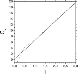
FIG. 13.: The specific heat $C_{v}$ as a function of the temperature calculated in the thermal SCRPA for $\Omega=N=50$. Solid line corresponds to $G=0.128$ ($\delta/\Delta=50$) and dotted line corresponds to $G=0.256$ ($\delta/\Delta=1$).

REFERENCES

• [1] D.C. Ralph, C.T. Black, and M. Tinkham, Phys. Rev. Lett. 74, 3241 (1995); D.C. Ralph, C.T. Black, and M. Tinkham, Phys. Rev. Lett. 76, 688 (1996); D.C. Ralph, C.T. Black, and M. Tinkham, Phys. Rev. Lett. 78, 4087 (1997).
• [2] J. von Delft and D.C. Ralph, Phys. Rep. 345, 61 (2001).
• [3] J. von Delft, Ann. Phys. (Leipzig) 10, 219 (2001).
• [4] R. Balian, H. Flocard, M. Veneroni, Phys. Rep. 317, 251 (1999).
• [5] P. Ring and P. Schuck, The Nuclear Many-Body Problem, (Springer-Verlag, NY, 1980).
• [6] R.W. Richardson and N. Sherman, Nucl. Phys. A52, 221 (1964).
• [7] B. Mühlschlegel, D.J. Scalapino, and R. Denton, Phys. Rev. B6, 1767, (1972).
• [8] A. Di Lorenzo et al., Phys. Rev. Lett. 84, 550 (2000); G. Falci, A. Fubini, A. Mastellone, Phys. Rev. B65, 140507(R), (2002).
• [9] R. Rossignoli, Phys. Rev. C54, 1230 (1996).
• [10] R. Rossignoli, N. Canosa and P. Ring, Phys. Rev. Lett. 80, 1853 (1998).
• [11] J. Bang and J. Krumlinde, Nucl. Phys. A141, 18 (1970); O. Civitarese, G.G. Dussel and R.P.J. Perazzo, Nucl. Phys. A404, 15 (1983); A. Kuriyama, J. Providencia, Y. Tsue and M. Yamamura, Prog. Theor. Phys. 105, 729 (2001).
• [12] G.D. Mahan, Many Particle Physics (Plenum Press, 1981).
• [13] J. Dukelsky, P. Schuck, Phys. Lett. B464 164 (1990); J.G. Hirsch, A. Mariano, J. Dukelsky and P. Schuck, Ann. Phys. (New York) 296, 187 (2002).
• [14] G. Röpke,T. Seifet, H. Stolz, R. Zimmermann, Phys. Stat. Sol. (b)100, 215 (1980); G. Röpke, Ann. Physik (Leipzig) 3, 145 (1994); G. Röpke, Z. Phys. B99, 83 (1995).
• [15] Ken-ji Hara, Prog. Theor. Phys. 32, 88 (1964); D.J. Rowe, Phys. Rev. 175, 1283 (1968); D.J. Rowe, Rev. Mod. Phys. 40, 153 (1968).
• [16] P. Schuck, Z. Physik 241, 395 (1971); P. Schuck, S. Ethofer, Nucl. Phys. A212, 269 (1973).
• [17] A.L. Fetter, J. D. Walecka, Quantum Theory of Many-Particle Systems, (McGraw-Hill, New York, 1971).
• [18] J. Dukelsky, G. Röpke and P. Schuck, Nucl. Phys. A628, 17 (1998).
• [19] A.B. Migdal, Theory of Finite Fermi Systems and Application to Atomic Nuclei, Monographs and Texts in Physics and Astronomy (Interscience publisher(Wiley), New York, 1967).
• [20] J. Dukelsky, P. Schuck, Phys. Lett. B464 164 (1990); J. Dukelsky, J.G. Hirsch, P. Schuck, Eur. Phys. J. A7 155 (2000).
• [21] P. Schuck et al., to be published.
• [22] A. Rabhi, R. Bennaceur, G. Chanfray, P. Schuck, nucl-th/0208037.
• [23] J. Dukelsky and G. Sierra, Phys. Rev. Lett., 83, 172 (1999).
• [24] A. Schnell, G. Röpke, P. Schuck, Phys. Rev. Lett. 83, 1926 (1999).
• [25] H. Ding et al., Nature (London) 382, 51 (1996); A.G. Loeser et al., Scince 273, 325 (1996).
• [26] N. Trivedi and M. Randeria, Phys. Rev. Lett. 75, 312 (1995).
• [27] R.V. Jolos and W. Rybarska, Z. Physik A 296, 73 (1980).
Refer to caption