Competition of ferromagnetic and antiferromagnetic
spin ordering in nuclear matter

Abstract

In the framework of a Fermi liquid theory it is considered the possibility of ferromagnetic and antiferromagnetic phase transitions in symmetric nuclear matter with Skyrme effective interaction. The zero temperature dependence of ferromagnetic and antiferromagnetic spin polarization parameters as functions of density is found for SkM^∗, SGII effective forces. It is shown that in the density domain, where both type of solutions of self–consistent equations exist, ferromagnetic spin state is more preferable than antiferromagnetic one.

I Introduction

The appearance of spontaneous spin polarized states in nuclear matter is the topic of a great current interest due to relevance in astrophysics. According as nuclear matter is spin polarized or not, drastically different scenarios of supernova explosion and cooling of neutron stars can be realized. The possibility of a phase transition of normal nuclear matter to ferromagnetic state was studied by many authors. In Ref. R within a hard sphere gas model it was shown that neutron matter becomes ferromagnetic at $\varrho\approx 0.41\,\mbox{fm}^{-3}$. In Refs. S ; O it was found that the inclusion of long–range attraction significantly increases the ferromagnetic transition density (e.g., up to $\varrho\approx 2.3\,\mbox{fm}^{-3}$ in the Brueckner theory with a simple central potential and hard core only for singlet spin states O ). Calculations of magnetic susceptibility in Ref. VNB with Skyrme effective forces showed that a ferromagnetic transition occurs at $\varrho\approx 0.18$–$0.26\,\mbox{fm}^{-3}$. The Fermi liquid criterion for the ferromagnetic instability in neutron matter with Skyrme interaction is reached at $\varrho\approx 2$–$4\varrho_{0}$ RPLP , $\varrho_{0}$ being nuclear matter saturation density. In Ref. ALP there were formulated general conditions on the parameters of neutron–neutron interaction, which result in the magnetically ordered state of neutron matter. The spin correlations in dense neutron matter within the relativistic Dirac–Hartree–Fock approach with the effective nucleon–meson Lagrangian were studied in Ref. MNQN , predicting the ferromagnetic transition at several times nuclear matter saturation density. The importance of the Fock exchange term in the relativistic mean–field approach for occurrence of ferromagnetism in nuclear matter was established in Ref. TT . The stability of strongly asymmetric nuclear matter with respect to spin fluctuations was investigated in Ref. KW , where it was shown that even small proton admixture favors the ferromagnetic instability of the system. This conclusion was confirmed also by calculations within the relativistic Dirac–Hartree–Fock approach to strongly asymmetric nuclear matter BMNQ .

If to consider the models with realistic nucleon–nucleon (NN) interaction, the ferromagnetic phase transition seems to be suppressed up to densities well above $\varrho_{0}$ PGS –H . In particular, no evidence of ferromagnetic instability has been found in recent studies of neutron matter VPR and asymmetric nuclear matter VB within the Brueckner–Hartree–Fock approximation with realistic Nijmegen II, Reid93 and Nijmegen NSC97e NN interactions. The same conclusion was obtained in Ref. FSS , where magnetic susceptibility of neutron matter was calculated with the use of the Argonne $v_{18}$ two–body potential plus Urbana IX three–body potential.

Here we will continue the study of spin polarizability of nuclear matter with the use of effective NN interaction. As a framework of consideration, it is chosen a Fermi liquid (FL) description of nuclear matter AKP ; AIP . As a potential of NN interaction, we use the Skyrme effective interaction, utilized earlier in a number of contexts for nuclear matter calculations SYK –AAI . Since calculations of magnetic susceptibility with the Skyrme effective forces show, that nuclear matter undergoes the ferromagnetic phase transition at some critical density, it is quite natural step to determine the density dependence of the ferromagnetic spin polarization parameter of nuclear matter. Besides, in this study we explore the possibility of antiferomagnetic phase transition in nuclear matter, when the spins of protons and neutrons are aligned in the opposite direction. The antiferromagnetic spin polarization parameter will be determined as a function of density as well. Then we study the question of thermodynamic stability of ferromagnetic and antiferromagnetic spin states and clarify which phase is thermodynamically preferable in the density region, where both solutions of self–consistent equations exist simultaneously.

Note that we consider thermodynamic properties of spin polarized states in nuclear matter up to the high density region relevant for astrophysics. Nevertheless, we use a pure nucleonic description of nuclear matter, although other degrees of freedom, such as pions, hyperons, kaons, or quarks could be present at such high densities.

II Basic Equations

Normal states of nuclear matter are described by the normal distribution function of nucleons $f_{\kappa_{1}\kappa_{2}}=\mbox{Tr}\,\varrho a^{+}_{\kappa_{2}}a_{\kappa_{1}}$ ($\kappa\equiv({\bf{p}},\sigma,\tau)$, ${\bf p}$ is momentum, $\sigma(\tau)$ is the projection of spin (isospin) on the third axis, $\varrho$ is the density matrix of the system). The energy of the system is specified as a functional of the distribution function $f$, $E=E(f)$, and determines the single particle energy

$$\varepsilon_{\kappa_{1}\kappa_{2}}(f)=\frac{\partial E(f)}{\partial f_{\kappa_{2}\kappa_{1}}}.$$ (1)

The self-consistent matrix equation for determining the distribution function $f$ follows from the minimum condition of the thermodynamic potential AKP and is

$$f=\left\{\mbox{exp}(Y_{0}\varepsilon+Y_{4})+1\right\}^{-1}\equiv\left\{\mbox{exp}(Y_{0}\xi)+1\right\}^{-1}.$$ (2)

Here the quantities $\varepsilon,Y_{4}$ are matrices in the space of $\kappa$ variables, with $Y_{4\kappa_{1}\kappa_{2}}=Y_{4\tau_{1}}\delta_{\kappa_{1}\kappa_{2}}$ $(\tau_{1}=p,n)$, $Y_{0}=1/T,\ Y_{4p}=-\mu_{p}^{0}/T$ and $Y_{4n}=-\mu_{n}^{0}/T$ the Lagrange multipliers, $\mu_{p}^{0}$ and $\mu_{n}^{0}$ the chemical potentials of protons and neutrons and $T$ the temperature. We shall study the possibility of formation of different types of spin ordering (ferromagnetic and antiferromagnetic) in nuclear matter.

The normal distribution function can be expanded in the Pauli matrices $\sigma_{i}$ and $\tau_{k}$ in spin and isospin spaces

$$f({\bf p}) =f_{00}({\bf p})\sigma_{0}\tau_{0}+f_{30}({\bf p})\sigma_{3}\tau_{0}$$ (3)

$$\quad+f_{03}({\bf p})\sigma_{0}\tau_{3}+f_{33}({\bf p})\sigma_{3}\tau_{3}.$$

For the energy functional, being invariant with respect to rotations in spin and isospin spaces, the structure of the single particle energy is similar to that of the distribution function $f$:

$$\varepsilon({\bf p}) =\varepsilon_{00}({\bf p})\sigma_{0}\tau_{0}+\varepsilon_{30}({\bf p})\sigma_{3}\tau_{0}$$ (4)

$$\quad+\varepsilon_{03}({\bf p})\sigma_{0}\tau_{3}+\varepsilon_{33}({\bf p})\sigma_{3}\tau_{3}.$$

Using Eqs. (2), (4), it is possible to express evidently the distribution functions $f_{00},f_{30},f_{03},f_{33}$ in terms of the quantities $\varepsilon$:

$$f_{00} =\frac{1}{4}\{n(\omega_{+,+})+n(\omega_{+,-})+n(\omega_{-,+})+n(\omega_{-,-})\},$$

$$f_{30} =\frac{1}{4}\{n(\omega_{+,+})+n(\omega_{+,-})-n(\omega_{-,+})-n(\omega_{-,-})\},$$

$$f_{03} =\frac{1}{4}\{n(\omega_{+,+})-n(\omega_{+,-})+n(\omega_{-,+})-n(\omega_{-,-})\},$$

$$f_{33} =\frac{1}{4}\{n(\omega_{+,+})-n(\omega_{+,-})-n(\omega_{-,+})+n(\omega_{-,-})\}.$$ (5)

Here $n(\omega)=\{\exp(Y_{0}\omega)+1\}^{-1}$ and

$$\omega_{+,+}=\xi_{00}+\xi_{30}+\xi_{03}+\xi_{33},\;$$

$$\omega_{+,-}=\xi_{00}+\xi_{30}-\xi_{03}-\xi_{33},\;$$

$$\omega_{-,+}=\xi_{00}-\xi_{30}+\xi_{03}-\xi_{33},\;$$

$$\omega_{-,-}=\xi_{00}-\xi_{30}-\xi_{03}+\xi_{33},\;$$

where

$$\xi_{00} =\varepsilon_{00}-\mu_{00}^{0},\;\xi_{30}=\varepsilon_{30},\;$$

$$\xi_{03} =\varepsilon_{03}-\mu_{03}^{0},\;\xi_{33}=\varepsilon_{33},$$

$$\mu_{00}^{0} ={\frac{\mu_{p}^{0}+\mu_{n}^{0}}{2}},\quad\mu_{03}^{0}={\frac{\mu_{p}^{0}-\mu_{n}^{0}}{2}}.$$

As follows from the structure of the distribution functions $f$, the quantity $\omega_{\pm,\pm}$, being the exponent in Fermi distribution function $n$, plays the role of the quasiparticle spectrum. In the considering case the spectrum is four–fold split due to spin and isospin dependence of the single particle energy $\varepsilon({\bf p})$ in Eq. (4). The distribution functions $f$ should satisfy the normalization conditions

$$\frac{4}{\cal V}\sum_{\bf p}f_{00}({\bf p}) =\varrho,$$ (6)

$$\frac{4}{\cal V}\sum_{\bf p}f_{03}({\bf p}) =\varrho_{p}-\varrho_{n}\equiv-\alpha\varrho,$$ (7)

$$\frac{4}{\cal V}\sum_{\bf p}f_{30}({\bf p}) =\varrho_{\uparrow}-\varrho_{\downarrow}\equiv\Delta\varrho_{\uparrow\uparrow},$$ (8)

$$\frac{4}{\cal V}\sum_{\bf p}f_{33}({\bf p}) =(\varrho_{p\uparrow}+\varrho_{n\downarrow})-(\varrho_{p\downarrow}+\varrho_{n\uparrow})\equiv\Delta\varrho_{\uparrow\downarrow}.$$ (9)

Here $\alpha$ is the isospin asymmetry parameter, $\varrho_{p\uparrow},\varrho_{p\downarrow}$ and $\varrho_{n\uparrow},\varrho_{n\downarrow}$ are the proton and neutron number densities with spin up and spin down, respectively; $\varrho_{\uparrow}=\varrho_{p\uparrow}+\varrho_{n\uparrow}$ and $\varrho_{\downarrow}=\varrho_{p\downarrow}+\varrho_{n\downarrow}$ are the nucleon densities with spin up and spin down. The quantities $\Delta\varrho_{\uparrow\uparrow}$ and $\Delta\varrho_{\uparrow\downarrow}$ may be regarded as ferromagnetic (FM) and antiferromagnetic (AFM) spin order parameters: if all nucleon spins are aligned in one direction (totally polarized FM spin state), then $\Delta\varrho_{\uparrow\uparrow}=\varrho$ and $\Delta\varrho_{\uparrow\downarrow}=0$; if spins of all protons are aligned in one direction and spins of all neutrons in the opposite one (totally polarized AFM spin state), then $\Delta\varrho_{\uparrow\downarrow}=\varrho$ and $\Delta\varrho_{\uparrow\uparrow}=0$.

To obtain the self–consistent equations, it is necessary to specify the energy functional of the system, which we write in the form

$$E(f) =E_{0}(f)+E_{int}(f),$$ (10)

$${E}_{0}(f) =4\sum\limits_{\bf p}\varepsilon_{0}({\bf p})f_{00}({\bf p}),\;\varepsilon_{0}({\bf p})=\frac{{\bf p}^{\,2}}{2m_{0}},$$

$${E}_{int}(f) =2\sum\limits_{\bf p}\{\tilde{\varepsilon}_{00}({\bf p})f_{00}({\bf p})+\tilde{\varepsilon}_{30}({\bf p})f_{30}({\bf p})$$

$$\quad+\tilde{\varepsilon}_{03}({\bf p})f_{03}({\bf p})+\tilde{\varepsilon}_{33}({\bf p})f_{33}({\bf p})\},$$

$$\tilde{\varepsilon}_{00}({\bf p}) =\frac{1}{2\cal V}\sum_{\bf q}U_{0}({\bf k})f_{00}({\bf q}),\;{\bf k}=\frac{{\bf p}-{\bf q}}{2},$$

$$\tilde{\varepsilon}_{30}({\bf p}) =\frac{1}{2\cal V}\sum_{\bf q}U_{1}({\bf k})f_{30}({\bf q}),$$

$$\tilde{\varepsilon}_{03}({\bf p}) =\frac{1}{2\cal V}\sum_{\bf q}U_{2}({\bf k})f_{03}({\bf q}),$$

$$\tilde{\varepsilon}_{33}({\bf p}) =\frac{1}{2\cal V}\sum_{\bf q}U_{3}({\bf k})f_{33}({\bf q}).$$

Here $m_{0}$ is the bare mass of a nucleon, $U_{0}({\bf k}),...,U_{3}({\bf k})$ are the normal FL amplitudes, $\tilde{\varepsilon}_{00},\tilde{\varepsilon}_{30},\tilde{\varepsilon}_{03},\tilde{\varepsilon}_{33}$ are the FL corrections to the free single particle spectrum. With allowance for Eqs. (1) and (10), we obtain the self–consistent equations in the form

$$\xi_{00}({\bf p}) = \varepsilon_{0}({\bf p})+\tilde{\varepsilon}_{00}({\bf p})-\mu_{00}^{0},\;\xi_{30}({\bf p})=\tilde{\varepsilon}_{30}({\bf p}),$$ (11)

$$\xi_{03}({\bf p}) = \tilde{\varepsilon}_{03}({\bf p})-\mu_{03}^{0},\;\xi_{33}({\bf p})=\tilde{\varepsilon}_{33}({\bf p}).$$

Further for obtaining numerical results we shall use the Skyrme effective interaction. In the case of Skyrme forces the normal FL amplitudes read AIP

$$U_{0}({\bf k}) =6t_{0}+t_{3}\varrho^{\beta}+\frac{2}{\hbar^{2}}[3t_{1}+t_{2}(5+4x_{2})]{\bf k}^{2},$$ (12)

$$U_{1}({\bf k}) =-2t_{0}(1-2x_{0})-\frac{1}{3}t_{3}\varrho^{\beta}(1-2x_{3})$$

$$\quad-\frac{2}{\hbar^{2}}[t_{1}(1-2x_{1})-t_{2}(1+2x_{2})]{\bf k}^{2}\equiv a+b{\bf k}^{2},$$

$$U_{2}({\bf k}) =-2t_{0}(1+2x_{0})-\frac{1}{3}t_{3}\varrho^{\beta}(1+2x_{3})$$

$$\quad-\frac{2}{\hbar^{2}}[t_{1}(1+2x_{1})-t_{2}(1+2x_{2})]{\bf k}^{2},$$

$$U_{3}({\bf k}) =-2t_{0}-\frac{1}{3}t_{3}\varrho^{\beta}-\frac{2}{\hbar^{2}}(t_{1}-t_{2}){\bf k}^{2}\equiv c+d{\bf k}^{2},$$

where $t_{i},x_{i},\beta$ are phenomenological constants, characterizing the given parametrization of Skyrme forces. In numerical calculations we shall use the SkM^∗ BGH and SGII SG potentials, developed to fit the properties of systems with small isospin asymmetry. With account of the evident form of FL amplitudes and Eqs. (6)–(9), one can obtain

$$\xi_{00} =\frac{p^{2}}{2m_{00}}-\mu_{00},$$ (13)

$$\xi_{03} =\frac{p^{2}}{2m_{03}}-\mu_{03},$$ (14)

$$\xi_{30} =(a+b\frac{{\bf p}^{2}}{4})\frac{\Delta\varrho_{\uparrow\uparrow}}{8}+\frac{b}{32}\langle{\bf q}^{2}\rangle_{30},$$ (15)

$$\xi_{33} =(c+d\frac{{\bf p}^{2}}{4})\frac{\Delta\varrho_{\uparrow\downarrow}}{8}+\frac{d}{32}\langle{\bf q}^{2}\rangle_{33},$$ (16)

where the effective nucleon mass $m_{00}$ and effective isovector mass $m_{03}$ are defined by the formulae:

$$\frac{\hbar^{2}}{2m_{00}} = \frac{\hbar^{2}}{2m_{0}}+\frac{\varrho}{16}[3t_{1}+t_{2}(5+4x_{2})],$$ (17)

$$\frac{\hbar^{2}}{2m_{03}} = \frac{\alpha\varrho}{16}[t_{1}(1+2x_{1})-t_{2}(1+2x_{2})],$$

and the renormalized chemical potentials $\mu_{00},\mu_{03}$ should be determined from Eqs. (6), (7). In Eqs. (15), (16) $\langle{\bf q}^{2}\rangle_{30},\langle{\bf q}^{2}\rangle_{33}$ are the second order moments of the corresponding distribution functions

$$\langle{\bf q}^{2}\rangle_{30} =\frac{4}{V}\sum_{\bf q}{\bf q}^{2}f_{30}({\bf q}),$$ (18)

$$\langle{\bf q}^{2}\rangle_{33} =\frac{4}{V}\sum_{\bf q}{\bf q}^{2}f_{33}({\bf q}).$$ (19)

Thus, with account of the expressions (5) for the distribution functions $f$, we obtain the self–consistent equations (6)–(9), (18), (19) for the effective chemical potentials $\mu_{00},\mu_{03}$, FM and AFM spin order parameters $\Delta\varrho_{\uparrow\uparrow}$, $\Delta\varrho_{\uparrow\downarrow}$, and the second order moments $\langle{\bf q}^{2}\rangle_{30},\langle{\bf q}^{2}\rangle_{33}$.

III Ferromagnetic and Antiferromagnetic spin order parameters at zero temperature

The early researches on spin polarizability with Skyrme effective interaction were based on the calculation of magnetic susceptibility and finding its pole structure VNB ; RPLP , determining the onset of instability with respect to spin fluctuations. Here we provide the direct calculation of FM spin polarization as a function of nuclear matter density at zero temperature. Besides, we study the possibility of AFM spin ordering in nuclear matter and competition between these two types of ordering.

Let us consider the zero temperature behavior of spin polarization in symmetric nuclear matter ($\varrho_{p}=\varrho_{n}$). The FM spin ordering corresponds to the case $\Delta\varrho_{\uparrow\uparrow}\not=0,\langle{\bf q}^{2}\rangle_{30}\not=0,\Delta\varrho_{\uparrow\downarrow}=0,\langle{\bf q}^{2}\rangle_{33}=0$, while the AFM spin ordering to the case $\Delta\varrho_{\uparrow\downarrow}\not=0,\langle{\bf q}^{2}\rangle_{33}\not=0,\Delta\varrho_{\uparrow\uparrow}=0,\langle{\bf q}^{2}\rangle_{30}=0$. In the totally ferromagnetically polarized state nontrivial solutions of the self–consistent equations have the form

$$\Delta\varrho_{\uparrow\uparrow}=\varrho,\;\langle{\bf q}^{2}\rangle_{30}=\frac{3}{5}\varrho k_{F}^{2}.$$ (20)

Here $k_{F}=(3\pi^{2}\varrho)^{1/3}$ is Fermi momentum of symmetric nuclear matter in the case when degrees of freedom, corresponding to spin up of nucleons, are open while those related to spin down are inaccessible. For totally antiferromagnetically polarized nuclear matter we have

$$\Delta\varrho_{\uparrow\downarrow}=\varrho,\;\langle{\bf q}^{2}\rangle_{33}=\frac{3}{5}\varrho k_{F}^{2}.$$ (21)

The Fermi momentum $k_{F}$ is given by the same expression as in Eq. (20) since now degrees of freedom, related to spin down of protons and spin up of neutrons, are inaccessible. The results of numerical determination of FM $\Delta\varrho_{\uparrow\uparrow}/\varrho$ and AFM $\Delta\varrho_{\uparrow\downarrow}/\varrho$ spin polarization parameters are shown in Fig. 1 for the SkM^∗ and SGII effective forces.

The FM spin order parameter arises at density $\varrho\approx 2\varrho_{0}$ for the SkM^∗ potential and at $\varrho\approx 2.75\varrho_{0}$ for the SGII potential. The AFM order parameter originates at $\varrho\approx 3.3\varrho_{0}$ for the SkM^∗ force and at $\varrho\approx 5\varrho_{0}$ for the SGII force. In both cases FM ordering appears earlier than AFM one. Nuclear matter becomes totally ferromagnetically polarized ($\Delta\varrho_{\uparrow\uparrow}/\varrho=1$) at density $\varrho\approx 2.7\varrho_{0}$ for the SkM^∗ force and at $\varrho\approx 3.9\varrho_{0}$ for the SGII force. Totally antiferromagnetically polarized state ($\Delta\varrho_{\uparrow\downarrow}/\varrho=1$) is formed at $\varrho\approx 4.5\varrho_{0}$ for the SkM^∗ potential and at $\varrho\approx 7.2\varrho_{0}$ for the SGII potential.

Note that the second order moments $\langle{\bf q}^{2}\rangle_{30},\langle{\bf q}^{2}\rangle_{33}$ of the distribution functions $f_{30},f_{33}$ play the role of the order parameters as well. In Fig. 2 it is shown behavior of these quantities normalized to their value in totally polarized state. The ratios $5\langle{\bf q}^{2}\rangle_{30}/3\varrho k_{F}^{2}$ and $5\langle{\bf q}^{2}\rangle_{33}/3\varrho k_{F}^{2}$ are regarded as FM and AFM order parameters, respectively. The behavior of these quantities is similar to that of the spin polarization parameters in Fig. 1, with the same values of the threshold densities for appearance and saturation of the order parameters.

In the density domain, where FM and AFM solutions of self–consistent equations exist simultaneously, it is necessary to clarify, which solution is thermodynamically preferable. With this purpose it is necessary to compare the free energies of both states. The results of the numerical calculation of the free energy density, measured from that of the normal state, are shown in Fig. 3. One can see, that for all relevant densities FM spin ordering is more preferable than AFM one, and, moreover, the difference between corresponding free energies becomes larger with increasing density, so that there is no evidence, that AFM spin ordering might become preferable at larger densities.

In conclusion, we have considered the possibility of spontaneous appearance of spin polarized states in symmetric nuclear matter, corresponding to FM and AFM spin ordering. The study has been done in the framework of a Fermi liquid description of nuclear matter, when nucleons interact via Skyrme effective forces (SkM^∗, SGII potentials). Unlike the previous considerations, where the possibility of formation of FM spin polarized states was studied on the base of calculation of magnetic susceptibility, we obtain the self–consistent equations for the FM and AFM spin polarization parameters and solve them in the case of zero temperature. It is shown that FM order parameter appears at densities $2$–$2.75\varrho_{0}$ and AFM one at densities $3.3$–$5\varrho_{0}$. In the density region, where both type of solutions exist, FM spin ordering wins competition for thermodynamic stability.

The author acknowledges the financial support of STCU (grant No. 1480).

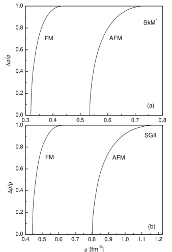
Figure 1: FM and AFM spin polarization parameters as functions of density at zero temperature for (a) SkM^∗ force and (b) SGII force.

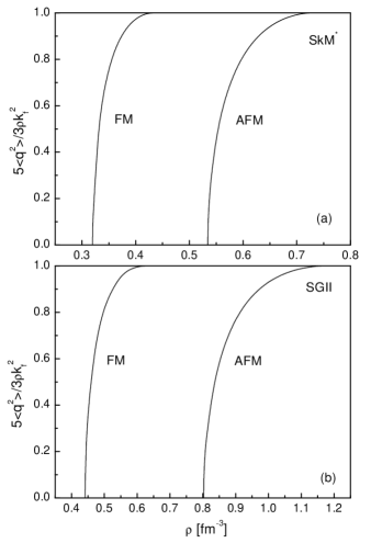
Figure 2: The same as in Fig. 1, but for the second order moments of the distribution functions.

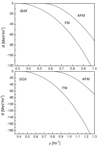
Figure 3: Free energy density, measured from that of the normal state, for FM and AFM spin ordering as function of density at zero temperature for (a) SkM^∗ force and (b) SGII force.

References

- (1) M.J. Rice, Phys. Lett. 29A, 637 (1969).
- (2) S.D. Silverstein, Phys. Rev. Lett. 23, 139 (1969).
- (3) E. Østgaard, Nucl. Phys. A154, 202 (1970).
- (4) A. Viduarre, J. Navarro, and J. Bernabeu, Astron. Astrophys. 135, 361 (1984).
- (5) S. Reddy, M. Prakash, J.M. Lattimer, and J.A. Pons, Phys. Rev. C 59, 2888 (1999).
- (6) A.I. Akhiezer, N.V. Laskin, and S.V. Peletminsky, Phys. Lett. 383B, 444 (1996).
- (7) S. Marcos, R. Niembro, M.L. Quelle, and J. Navarro, Phys. Lett. 271B, 277 (1991).
- (8) T. Maruyama and T. Tatsumi, Nucl. Phys. A693, 710 (2001).
- (9) M. Kutschera, and W. Wojcik, Phys. Lett. 223B, 11 (1989).
- (10) P. Bernardos, S. Marcos, R. Niembro, and M.L. Quelle, Phys. Lett. 356B, 175 (1995).
- (11) V.R. Pandharipande, V.K. Garde, and J.K. Srivatsava, Phys. Lett. 38B, 485 (1972).
- (12) S.O. Bäckmann and C.G. Källman, Phys. Lett. 43B, 263 (1973).
- (13) P. Haensel, Phys. Rev. C 11, 1822 (1975).
- (14) I. Vidaa, A. Polls, and A. Ramos, Phys. Rev. C 65, 035804 (2002).
- (15) I. Vidaa, and I. Bombaci, Phys. Rev. C 66, 045801 (2002).
- (16) S. Fantoni, A. Sarsa, and E. Schmidt, Phys. Rev. Lett. 87, 018110 (2001).
- (17) A.I. Akhiezer, V.V. Krasil’nikov, S.V. Peletminsky, and A.A. Yatsenko, Phys. Rep. 245, 1 (1994).
- (18) A.I. Akhiezer, A.A. Isayev, S.V. Peletminsky, A.P. Rekalo, and A.A. Yatsenko, Sov. Phys. JETP 85, 1 (1997).
- (19) R.K. Su, S.D. Yang, and T.T.S. Kuo, Phys. Rev. C 35, 1539 (1987).
- (20) M.F. Jiang and T.T.S. Kuo, Nucl. Phys. A481, 294 (1988).
- (21) A.I. Akhiezer, A.A. Isayev, S.V. Peletminsky, and A.A. Yatsenko, Phys. Rev. C 63, 021304(R) (2001).
- (22) A.A. Isayev, Phys. Rev. C 65, 031302(R) (2002).
- (23) M. Brack, C. Guet and H.-B. Hakansson, Phys. Rep. 123, 275 (1985).
- (24) V.G. Nguyen, and H. Sagawa, Phys. Lett. 106B, 379 (1981).