Deuteron distribution in nuclei and the Levinger’s factor

Abstract

We compute the distribution of quasideuterons in doubly closed shell nuclei. The ground states of ¹⁶O and ⁴⁰Ca are described in $ls$ coupling using a realistic hamiltonian including the Argonne $v_{8}^{\prime}$ and the Urbana IX models of two– and three–nucleon potentials, respectively. The nuclear wave function contains central and tensor correlations, and correlated basis functions theory is used to evaluate the distribution of neutron-proton pairs, having the deuteron quantum numbers, as a function of their total momentum. By computing the number of deuteron–like pairs we are able to extract the Levinger’s factor and compare to both the available experimental data and the predictions of the local density approximation, based on nuclear matter estimates. The agreement with the experiments is excellent, whereas the local density approximation is shown to sizably overestimate the Levinger’s factor in the region of the medium nuclei.

I Introduction

Within the Levinger’s quasideuteron (QD) model [1, 2, 3] the nuclear photoabsorption cross section $\sigma_{A}(E_{\gamma})$, above the giant dipole resonance and below pion threshold, is assumed to be proportional to the break-up cross section of a deuteron in hadronic matter, $\sigma_{QD}(E_{\gamma})$:

$$\sigma_{A}(E_{\gamma})={\mathcal{P}_{D}}\ \sigma_{QD}(E_{\gamma})\ ,$$ (1)

where $E_{\gamma}$ is the photon energy and $\mathcal{P}_{D}$ is interpreted as the effective number of the nucleon–nucleon (NN) pairs of the QD type (see [4] and references therein ). $\mathcal{P}_{D}$ is written in the form

$${\mathcal{P}_{D}}={\mathrm{L}}\ \left[\dfrac{Z({A-Z})}{A}\right]\ ,$$ (2)

where $A$ and $Z$ are the mass and atomic numbers of the nucleus and $\mathrm{L}$ is the so called Levinger’s factor. $\mathcal{P}_{D}$ can be calculated for a given nuclear ground state wave function, thus allowing for a microscopic interpretation of the phenomenological Levinger’s factor.

The value of $\mathrm{L}$ has been extracted from experiments according to the following two models: i) the Levinger’s model[5], in which $\sigma_{QD}(E_{\gamma})$ is taken as the deuteron cross section damped by an exponential function, taking care of Pauli blocking of the final states available to the nucleon ejected from the QD, and ii) the Laget’s model[6], which associates $\sigma_{QD}(E_{\gamma})$ with the transition amplitudes of virtual ($\pi\ +\ \rho$)–meson exchanges between the two nucleons of the QD pair.

Both models provide satisfactory fits of photoreaction data in heavy nuclei, but yield different values of the Levinger’s factor, ${\mathrm{L}}_{\text{Lev}}(A)$ and ${\mathrm{L}}_{\text{Laget}}(A)$, ${\mathrm{L}}_{\text{Laget}}(A)$ being $\sim 20\%$ larger than ${\mathrm{L}}_{\text{Lev}}(A)$.

The effective number of deuteron-like pairs, as well as of three- and four-body structures, in spherical nuclei has been investigated within the shell model approach in Refs.[7, 8]. In a recent paper [9] (referred to as I hereafter) we have analyzed the properties of deuteron-like structures in infinite symmetric nuclear matter (NM), described by a hamiltonian containing the realistic Urbana $v_{14}$ NN potential and the Urbana TNI many-body potential [10]. A correlated wave function having spin-isospin dependent, central and tensor correlations has been used within the correlated basis functions (CBF) theory to compute the QD distribution function in matter and extract the NM Levinger’s factor at equilibrium density, ${\mathrm{L}}_{NM}=11.63$, to be compared to the empirical estimate, ${\mathrm{L}}_{\text{expt}}(A=\infty)=9.26$.

CBF theory has established itself as one of the most effective tools to realistically study, from a microscopic viewpoint, properties of infinite matter of nucleons ranging from the equation of state [11, 12] to the momentum distribution [13] and the one– and two–body Green’s functions [14, 15, 16, 17]. In the last decade these studies have been successfully extended to deal with finite nuclei [18, 19, 20, 21, 22].

In this paper we extend the CBF many body approach, used in I for NM, to evaluate ab initio the momentum distribution, $P_{D}({{\mathbf{k}}}_{D})$, and the total number per particle, ${\mathcal{P}_{D}}/A$, of QD pairs in the doubly closed shell nuclei ¹⁶O and ⁴⁰Ca, described in the $ls$ coupling scheme. From ${\mathcal{P}_{D}}/A$ we then extract the corresponding Levinger’s factors.

In Section II we review and generalize the CBF approach to the QD distribution in terms of the overlap between the nuclear and deuteron ground state wave functions. In Section III we compute the QD distribution and $\mathcal{P}_{D}$ in nuclei described by a realistic hamiltonian including the modern Argonne $v^{\prime}_{8}$ [23] and the Urbana IX [24] models of two– and three–nucleon potentials, respectively. The correlated nuclear wave function contains central and tensor correlations, as in Ref. [21]. The results are compared with the analogous NM quantities, obtained in I. We also evaluate the Levinger’s factors, and compare them to the experimental values, as well as to those derived using the local density approximation (LDA) and the NM results of I. Summary and conclusions are given in Section. IV.

II Quasideuteron distribution

Following the approach developed in I, in a $A$–nucleon system the distribution of QD pairs whose center of mass is in the orbital state specified by the quantum number $X$ can be written

$$P_{D}(X)=\dfrac{1}{2J_{D}+1}\langle A|(a^{\alpha}_{D})^{\dagger}(X)a_{D}^{\alpha}(X)|A\rangle\,,$$ (3)

where $|A\rangle$ denotes the $A$–body ground state and $J_{D}=1$ is the spin of the deuteron. The operator $a(a^{\dagger})^{\alpha}_{D}(X)$ annihililates (creates) a deuteron with the quantum number $X$ in the $\alpha=1,2,3$ cartesian state. By introducing a complete set of intermediate $(A-2)$– particle states and exploiting the completeness relation $\sum_{n}|n(A-2)\rangle\langle n(A-2)|=1$, we can recast Eq.(3) in the form

$$P_{D}(X)=\dfrac{1}{2J_{D}+1}\sum_{n}\langle A|(a^{\alpha}_{D})^{\dagger}(X)|n(A-2)\rangle\langle n(A-2)|a_{D}^{\alpha}(X)|A\rangle\,.$$ (4)

In configuration space the above expression takes the form:

$$P_{D}(X) =\dfrac{1}{2J_{D}+1}\dfrac{A(A-1)}{2}$$ (5)

$$\int d{\widetilde{R}}d^{3}r_{1}d^{3}r_{2}d^{3}r_{1^{\prime}}d^{3}r_{2^{\prime}}\Psi_{A}^{\ast}({{\mathbf{r}}}_{1},{{\mathbf{r}}}_{2},{\widetilde{R}})\Psi_{D}^{\alpha}(X;{{\mathbf{r}}}_{1},{{\mathbf{r}}}_{2})\left(\Psi_{D}^{\alpha}(X;{{\mathbf{r}}}_{1^{\prime}},{{\mathbf{r}}}_{2^{\prime}})\right)^{\ast}\Psi_{A}({{\mathbf{r}}}_{1^{\prime}},{{\mathbf{r}}}_{2^{\prime}},{\widetilde{R}})\ ,$$ (6)

where ${\widetilde{R}}\equiv({{\mathbf{r}}}_{3},\ldots,{{\mathbf{r}}}_{A})$, $\Psi_{A}$ is the normalized nuclear ground state wave function and $\Psi_{D}^{\alpha}$ is the deuteron wave function (DWF).

The DWF can be split into its center of mass and relative motion parts according to

$$\Psi_{D}^{\alpha}(X;{{\mathbf{r}}}_{i},{{\mathbf{r}}}_{j})=\Psi_{D,cm}(X;{{\mathbf{R}}}_{ij})\ \psi^{\alpha}_{D,rel}(ij)|00\rangle\ ,$$ (7)

where ${{\mathbf{R}}}_{ij}=({{\mathbf{r}}}_{i}+{{\mathbf{r}}}_{j})/2$, ${{\mathbf{r}}}_{ij}={{\mathbf{r}}}_{i}-{{\mathbf{r}}}_{j}$, $|00\rangle$ is the spin–isospin singlet NN state and

$$\psi^{\alpha}_{D,rel}(ij)=\left[u_{D}(r_{ij})\sigma_{i}^{\alpha}-\dfrac{w_{D}(r_{ij})}{\sqrt{2}}T^{\alpha\beta}(\widehat{{{\mathbf{r}}}}_{ij})\sigma_{i}^{\beta}\right]\ .$$ (8)

$u_{D}(r)$ and $w_{D}(r)$ being the $\ell=0$ and $\ell=2$ components of the deuteron wave function, whose normalization is given by

$$\int_{0}^{\infty}r^{2}dr\left[u_{D}^{2}(r)+w_{D}^{2}(r)\right]=1\ ,$$ (9)

In Eq.(8) $\sigma_{i}^{\alpha}$ are the spin Pauli matrices, while the tensor operator reads

$$T^{\alpha\beta}(\widehat{{{\mathbf{r}}}}_{ij})=3\widehat{{{\mathbf{r}}}}_{ij}^{\alpha}\widehat{{{\mathbf{r}}}}_{ij}^{\beta}-\delta^{\alpha\beta}\ .$$ (10)

Using the above definitions $P_{D}(X)$ can finally be rewritten as:

$$P_{D}(X) =\dfrac{1}{2J_{D}+1}\dfrac{1}{2}$$ (11)

$$\int d^{3}r_{1}d^{3}r_{2}d^{3}r_{1^{\prime}}d^{3}r_{2^{\prime}}\Psi_{D,cm}(X;{{\mathbf{R}}}_{12})\rho^{(2)}_{D}({{\mathbf{r}}}_{1},{{\mathbf{r}}}_{2};{{\mathbf{r}}}_{1^{\prime}},{{\mathbf{r}}}_{2^{\prime}})\Psi^{\ast}_{D,cm}(X;{{\mathbf{R}}}_{1^{\prime}2^{\prime}})\,,$$ (12)

where $\rho^{(2)}_{D}({{\mathbf{r}}}_{1},{{\mathbf{r}}}_{2};{{\mathbf{r}}}_{1^{\prime}},{{\mathbf{r}}}_{2^{\prime}})$ is a generalized two–body density matrix defined by

$$\rho^{(2)}_{D}({{\mathbf{r}}}_{1},{{\mathbf{r}}}_{2};{{\mathbf{r}}}_{1^{\prime}},{{\mathbf{r}}}_{2^{\prime}}) =A(A-1)$$ (13)

$$\int d{\widetilde{R}}\,\Psi_{A}^{\ast}({{\mathbf{r}}}_{1},{{\mathbf{r}}}_{2},{\widetilde{R}})\psi_{D,rel}^{\alpha}(12)|00\rangle\langle 00|\left(\psi_{D,rel}^{\alpha}(1^{\prime}2^{\prime})\right)^{\ast}\Psi_{A}({{\mathbf{r}}}_{1^{\prime}},{{\mathbf{r}}}_{2^{\prime}},{\widetilde{R}})\,,$$ (14)

where summation over the repeated indices is understood.

The sum over $X$ yields the total number of QD pairs in the nucleus, $\mathcal{P}_{D}$, thus allowing for a direct estimate of the Levinger’s factor, $\mathrm{L}$, to be compared to the empirical values resulting from phenomenological analyses [25, 26] of photoreaction data [27, 28].

A realistic $A$–body wave function, accounting for both short– and intermediate–range correlations induced by the strong nuclear interaction, is given in CBF theory by

$$\Psi_{A}(R)={\mathcal{S}}\Bigl{[}\prod_{i<j}F(ij)\Bigl{]}\Phi_{0}(R)\,,$$ (15)

where $R\equiv({{\mathbf{r}}}_{1},\ldots,{{\mathbf{r}}}_{A})$, $\mathcal{S}$ is a symmetrization operator and $\Phi_{0}$ is the Slater determinant of single particle orbitals $\phi_{\alpha}(i)$, which are eigenfunctions of a suitable single particle hamiltonian. For nuclear matter, the orbitals $\phi_{\alpha}(i)$ are plane waves corresponding to a noninteracting Fermi gas of nucleons with momenta $|{{\mathbf{k}}}|\leq k_{F}=(6\pi^{2}\rho_{NM}/\nu)^{1/3}$, $\nu=4$ and $\rho_{NM}$ are the NM spin–isospin degeneracy and density, respectively.

The two–body correlation operator, $F(ij)$, is given by the sum of 6 central and non–central spin–isospin dependent components,

$$F(ij)=f_{c}(r_{ij})+f_{\sigma}(r_{ij})(\boldsymbol{\sigma}_{i}\cdot\boldsymbol{\sigma}_{j})+f_{\tau}(r_{ij})(\boldsymbol{\tau}_{i}\cdot\boldsymbol{\tau}_{j})+f_{\sigma\tau}(r_{ij})(\boldsymbol{\sigma}_{i}\cdot\boldsymbol{\sigma}_{j})(\boldsymbol{\tau}_{i}\cdot\boldsymbol{\tau}_{j})$$ (16)

$$+f_{t}(r_{ij})T_{\alpha\beta}(\widehat{{{\mathbf{r}}}}_{ij})\sigma_{i}^{\alpha}\sigma_{j}^{\beta}+f_{t\tau}(r_{ij})T_{\alpha\beta}(\widehat{{{\mathbf{r}}}}_{ij})\sigma_{i}^{\alpha}\sigma_{j}^{\beta}(\boldsymbol{\tau}_{i}\cdot\boldsymbol{\tau}_{j})\ ,$$ (17)

where the $f_{p}(r)$ correlation functions are variationally fixed by minimizing the ground state energy [21, 29, 30]. All the correlation functions heal to zero, except $f_{c}(r\rightarrow\infty)\rightarrow 1$.

The generalized two–body density matrix $\rho^{(2)}_{D}$ can be expanded in a series of terms involving an increasing number of nucleons by means of cluster expansion techniques [31]. In I the dressed leading order approximation (corresponding to the cluster diagram shown in Fig. 1 of I) was used to evaluate the momentum distribution of QD pairs in nuclear matter. The validity of this approximation has been satisfactorily checked in CBF calculations of the NM responses [32, 33] and Green’s functions [14, 15]. In Ref. [22] the one–body density matrix of the $N=Z$ doubly closed shell nuclei ¹⁶O and ⁴⁰Ca has been computed using the correlation operator of Eq. (17), the realistic Argonne $v^{\prime}_{8}$+Urbana IX interaction and the Fermi hypernetted chain/single operator chain (FHNC/SOC) diagrams resummation method [29, 30]. Here we extend the approximation employed to calculate $\rho^{(2)}_{D}$ in I to these two nuclei.

In the dressed leading order approximation $\rho^{(2)}_{D}({{\mathbf{r}}}_{1},{{\mathbf{r}}}_{2};{{\mathbf{r}}}_{1^{\prime}},{{\mathbf{r}}}_{2^{\prime}})$ is given by

$$\rho^{(2)}_{D}({{\mathbf{r}}}_{1},{{\mathbf{r}}}_{2};{{\mathbf{r}}}_{1^{\prime}},{{\mathbf{r}}}_{2^{\prime}})\approx\dfrac{2J_{D}+1}{4\pi}\rho^{(1)}({{\mathbf{r}}}_{1},{{\mathbf{r}}}_{1^{\prime}})\Sigma({{\mathbf{r}}}_{12},{{\mathbf{r}}}_{1^{\prime}2^{\prime}})\rho^{(1)}({{\mathbf{r}}}_{2},{{\mathbf{r}}}_{2^{\prime}})\,,$$ (18)

where $\rho^{(1)}({{\mathbf{r}}}_{1},{{\mathbf{r}}}_{1^{\prime}})$ is the one–body density matrix [22] and

$$\Sigma({{\mathbf{r}}}_{12},{{\mathbf{r}}}_{1^{\prime}2^{\prime}})=\dfrac{1}{3}{\mathrm{T}r}\left[F^{\dagger}(1^{\prime}2^{\prime})\psi_{D,rel}^{\alpha\dagger}(1^{\prime}2^{\prime})\Pi_{00}\psi_{D,rel}^{\alpha}(12)F(12)\left(1-P_{\sigma}P_{\tau}\right)\right]\ .$$ (19)

$\Pi_{00}$ and $P_{\sigma}P_{\tau}$ are the projector onto the $(ST)=(00)$ two–nucleon state and the spin–isospin exchange operator, respectively (see I for details).

By explicitly evaluating the trace in Eq. (19) in spin–isospin saturated systems, one gets

$$\Sigma({{\mathbf{r}}},{{\mathbf{r}}}^{\prime})=\dfrac{1}{16}\left[U(r)U(r^{\prime})+W(r)W(r^{\prime})Q(\widehat{{{\mathbf{r}}}}\cdot\widehat{{{\mathbf{r}}}}^{\prime})\right]\,,$$ (20)

with $Q(x)=(3x^{2}-1)/2$, $U(r)=u_{D}(r)-\Delta u(r)$ and $W(r)=w_{D}(r)-\Delta w(r)$. The $\Delta u(r)$ and $\Delta w(r)$ functions account for the medium correlations effect on the bare components of the DWF. Their explicit expressions, in terms of the correlation functions, are given in I.

Similarly to what is done to obtain the one–body momentum distribution in a nucleus, we consider the c.m. orbital to be a plane wave with momentum ${{\mathbf{k}}}_{D}$ in a periodical box of volume $\Omega$,

$$\Psi_{D,cm}({{\mathbf{k}}}_{D};{{\mathbf{R}}}_{ij})=\dfrac{{\mathrm{e}}^{i{{\mathbf{k}}}_{D}\cdot{{\mathbf{R}}}_{ij}}}{\sqrt{\Omega}}\,.$$ (21)

As a consequence, for the QD momentum distribution (MD) we get:

$${\mathcal{P}_{D}}({{\mathbf{k}}}_{D}) =\Omega\,P_{D}({{\mathbf{k}}}_{D})$$ (22)

$$=\dfrac{1}{2}\dfrac{1}{4\pi}\int d^{3}r_{1}d^{3}r_{2}d^{3}r_{1^{\prime}}d^{3}r_{2^{\prime}}\ {\mathrm{e}}^{i{{\mathbf{k}}}_{D}\cdot({{\mathbf{R}}}_{12}-{{\mathbf{R}}}_{1^{\prime}2^{\prime}})}\rho^{(1)}({{\mathbf{r}}}_{1},{{\mathbf{r}}}_{1^{\prime}})\Sigma({{\mathbf{r}}}_{12},{{\mathbf{r}}}_{1^{\prime}2^{\prime}})\rho^{(1)}({{\mathbf{r}}}_{2},{{\mathbf{r}}}_{2^{\prime}})\,.$$ (23)

This expression reduces to Eq. (13) of I in nuclear matter. Note that, in principle, different basis functions for the c.m. orbitals, describing the spatial distribution of deuteron–like clusters inside the nucleus, can be used.

In order to evaluate ${\mathcal{P}_{D}}({{\mathbf{k}}}_{D})$ we define the function $N({{\mathbf{r}}}_{1},{{\mathbf{r}}}_{1^{\prime}})$ through the relation [22]

$$\rho^{(1)}({{\mathbf{r}}}_{1},{{\mathbf{r}}}_{1^{\prime}})=N({{\mathbf{r}}}_{1},{{\mathbf{r}}}_{1^{\prime}})\sum_{\sigma\tau}\chi^{\dagger}_{\sigma\tau}(1)\chi_{\sigma\tau}(1^{\prime})\,,$$ (24)

where $\chi_{\sigma\tau}(1)$ is the spin–isospin single particle wave function. ${\mathcal{P}_{D}}({{\mathbf{k}}}_{D})$ can be written in terms of the Fourier transforms of $N$, $U$ and $W$ as

$${\mathcal{P}_{D}}({{\mathbf{k}}}_{D}) =\dfrac{\nu^{2}}{16}\,\dfrac{(2\pi)^{3}}{4\pi}\,\int d^{3}kd^{3}k^{\prime}$$ (25)

$$N\left(\dfrac{{{\mathbf{k}}}_{D}}{2}-{{\mathbf{k}}},\dfrac{{{\mathbf{k}}}_{D}}{2}+{{\mathbf{k}}}^{\prime}\right)\left[U(k)U(k^{\prime})+W(k)W(k^{\prime})Q(\widehat{{{\mathbf{k}}}}\cdot\widehat{{{\mathbf{k}}}}^{\prime})\right]N\left(\dfrac{{{\mathbf{k}}}_{D}}{2}+{{\mathbf{k}}},\dfrac{{{\mathbf{k}}}_{D}}{2}-{{\mathbf{k}}}^{\prime}\right)\,.$$ (26)

$N({{\mathbf{k}}},{{\mathbf{k}}}^{\prime})$ is related to $N({{\mathbf{r}}},{{\mathbf{r}}}^{\prime})$ through

$$N({{\mathbf{r}}},{{\mathbf{r}}}^{\prime})=\dfrac{1}{(2\pi)^{3}}\,\int d^{3}kd^{3}k^{\prime}\,{\mathrm{e}}^{-i({{\mathbf{k}}}\cdot{{\mathbf{r}}}-{{\mathbf{k}}}^{\prime}\cdot{{\mathbf{r}}}^{\prime})}\,N({{\mathbf{k}}},{{\mathbf{k}}}^{\prime})\,,$$ (27)

and $U(k)$ and $W(k)$ are given in I.

In spherically symmetric nuclei spin and isospin indices are saturated and $N({{\mathbf{k}}},{{\mathbf{k}}}^{\prime})$ can be expressed in terms of Fourier–like transforms of the natural orbits (NO), $\phi_{nl}^{NO}(k)$ [22]:

$$N({{\mathbf{k}}},{{\mathbf{k}}}^{\prime})=\sum_{n,l}\dfrac{2l+1}{4\pi}P_{l}(\widehat{{{\mathbf{k}}}}\cdot\widehat{{{\mathbf{k}}}}^{\prime})\,n_{nl}\,\phi_{nl}^{NO}(k)\,\phi_{nl}^{NO}(k^{\prime})\ ,$$ (28)

where $P_{l}(x)$ denotes the $l$-th Legendre polynomial and $\phi_{nl}^{NO}(k)$ is related to the configuration space NO, $\phi_{nl}^{NO}(r)$, through

$$\phi_{nl}^{NO}(k)=(2\pi)^{-3/2}\,\int d^{3}r\,j_{l}(kr)\,\phi_{nl}^{NO}(r)\ ,$$ (29)

$j_{l}(kr)$ being the spherical Bessel functions of order $l$.

The NO and their occupation numbers, $n_{nl}$, are obtained by first expanding the one–body density matrix in multipoles,

$$\rho^{(1)}({{\mathbf{r}}}_{1},{{\mathbf{r}}}_{1^{\prime}})=\sum_{l}\dfrac{2l+1}{4\pi}P_{l}(\widehat{{{\mathbf{r}}}}\cdot\widehat{{{\mathbf{r}}}}^{\prime})\rho^{(1)}_{l}(r_{1},r_{1^{\prime}})\,,$$ (30)

and then diagonalizing $\rho^{(1)}_{l}(r_{1},r_{1^{\prime}})$,

$$\rho^{(1)}_{l}(r_{1},r_{1^{\prime}})=\nu\sum_{n}n_{nl}\,\phi_{nl}^{NO}(r_{1})\,\phi_{nl}^{NO}(r_{1^{\prime}})\,.$$ (31)

The NO normalization is

$$1\,=\,\int r^{2}\,dr|\phi_{nl}^{NO}(r)|^{2}\,=\,\int k^{2}\,dk|\phi_{nl}^{NO}(k)|^{2}\,.$$ (32)

In the independent particle model (IPM), $\Psi_{A}(R)\equiv\Phi_{0}(R)$, and $n_{nl}^{IPM}=1$, $\phi_{nl}^{NO}\equiv\phi_{nl}$ for occupied states, whereas $n_{nl}^{IPM}=0$ for unoccupied states. Deviations from IPM provide a measure of correlation effects, as they allow higher NO to become populated with $n_{nl}\neq 0$.

Using Eq. (28) we obtain:

$${\mathcal{P}_{D}}({{\mathbf{k}}}_{D})=\sum_{\alpha,\alpha^{\prime}}\,n_{\alpha}n_{\alpha^{\prime}}\,{\mathcal{P}}_{\mathcal{D}}^{\alpha,\alpha^{\prime}}({{\mathbf{k}}}_{D})\,,$$ (33)

with

$${\mathcal{P}}_{\mathcal{D}}^{\alpha,\alpha^{\prime}}({{\mathbf{k}}}_{D})=\dfrac{\nu^{2}}{16}\,\dfrac{(2\pi)^{3}}{4\pi}\,\left[|\Psi^{\alpha,\alpha^{\prime}}_{S}({{\mathbf{k}}}_{D})|^{2}\,+\sum_{s=-2}^{2}|\Psi^{\alpha,\alpha^{\prime};\,s}_{D}({{\mathbf{k}}}_{D})|^{2}\right]\,,$$ (34)

where $\alpha=(nlm)$,

$$\Psi^{\alpha,\alpha^{\prime}}_{S}({{\mathbf{k}}}_{D})=\int d^{3}k\,\phi_{\alpha}^{NO\dagger}\left(\dfrac{{{\mathbf{k}}}_{D}}{2}+{{\mathbf{k}}}\right)\,U(k)\,\phi_{\alpha^{\prime}}^{NO}\left(\dfrac{{{\mathbf{k}}}_{D}}{2}-{{\mathbf{k}}}\right)\,,$$ (35)

$$\Psi^{\alpha,\alpha^{\prime};\,s}_{D}({{\mathbf{k}}}_{D})=\sqrt{\dfrac{4\pi}{5}}\int d^{3}k\,\phi_{\alpha}^{NO\dagger}\left(\dfrac{{{\mathbf{k}}}_{D}}{2}+{{\mathbf{k}}}\right)\,W(k)\,\phi_{\alpha^{\prime}}^{NO}\left(\dfrac{{{\mathbf{k}}}_{D}}{2}-{{\mathbf{k}}}\right)\,Y_{2s}(\widehat{{{\mathbf{k}}}})\,,$$ (36)

and

$$\phi_{nlm}^{NO}({{\mathbf{q}}})=\phi_{nl}^{NO}(q)\,Y_{lm}(\widehat{{{\mathbf{q}}}})\,,$$ (37)

$Y_{lm}(\widehat{{{\mathbf{q}}}})$ being the spherical harmonics.

III Results

Last generation NN potentials are able to fit deuteron properties and the Nijmegen 93 nucleon–nucleon scattering phase-shifts[36] up to the pion–production threshold ($\sim 4000$ data points) with a $\chi^{2}\sim 1$. The Argonne $v_{18}$, belonging to this generation, is given by the sum of 14 isoscalar and 4 isovector terms, including charge-symmetry and charge-invariance breaking components[23]. In this work we have used a simpler NN potential, referred to as Argonne $v_{8}^{\prime}$, obtained from the the full Argonne $v_{18}$ retaining only the first eight operatorial terms, corresponding to those shown in Eq. (17) plus spin–orbit and spin–orbit/isospin. The Argonne $v_{8}^{\prime}$ is constructed in such a way to reproduce the isoscalar part of the full $v_{18}$ in the $S$, $P$ and ${}^{3}D_{1}$ waves and the ${}^{3}D_{1}$–${}^{3}S_{1}$ coupling. The $v_{8}^{\prime}$ parameterization, while allowing for a fully realistic NN interaction, makes the use of modern many-body methods, like CBF [21, 34] or quantum Monte Carlo simulations [24, 35] much more practical. It has been found that the differences between Argonne $v_{8}^{\prime}$ and the full $v_{18}$ contribute very little to the binding energy of light nuclei and nuclear matter, and can be safely estimated either by perturbation theory or from FHNC/SOC calculations.

It is well known that, to quantitatively describe the properties of nuclei with $A>2$, modern NN interactions need to be supplemented with three-body forces. The Urbana IX (UIX) model provides a very good description of the energies of both the ground and the low-lying excited states of light nuclei ($A\leq 8$). In the present calculations we use Argonne $v_{8}^{\prime}$ + UIX interaction, which will be referred to as as the AU8^′ model. This interaction has already been used in the variational FHNC/SOC calculations of Ref. [22] as well as in the quantum Monte Carlo simulations of Ref. [24].

For the single particle wave functions, $\phi_{\alpha}(i)$, entering the shell model wave function $\Phi_{0}$, we have solved the single particle Schrödinger equation with a Woods–Saxon potential,

$$V_{WS}(r)=\dfrac{V_{0}}{1+\exp{[(r-R_{0})/a_{0}]}}\,.$$ (38)

In principle, the parameters of the correlation functions, $f_{p}(r)$, and of the Woods–Saxon potential may be both fixed by minimizing the ground state energy. This complete minimization was performed for the AU8^′ model in Ref. [21], and provided a binding energy per nucleon of $B/A=5.48~{}\text{MeV}$ in ¹⁶O and $B/A=6.97~{}\text{MeV}$ in ⁴⁰Ca (the experimental values are $7.97~{}\text{MeV}$ in ¹⁶O and $8.55~{}\text{MeV}$ in ⁴⁰Ca). These differences are compatible with the results of nuclear matter calculations at saturation density, $\rho_{NM}=0.16~{}\text{fm}^{-3}$, carried out with the same hamiltonian. In fact, the FHNC/SOC nuclear matter energy per nucleon is $E_{NM}/A=-10.9~{}\text{MeV}$ [21], to be compared to the empirical value of $-16~{}\text{MeV}$.

However, the calculated root mean square radii of the two nuclei turned out to be $R=2.83~{}\text{fm}$ in ¹⁶O and $R=3.66~{}\text{fm}$ in ⁴⁰Ca, showing a difference of $\sim 5\%$ with the experimental values, $R_{\text{expt}}=2.73~{}\text{fm}$ and $R_{\text{expt}}=3.48~{}\text{fm}$, respectively. Moreover, the one–body densities were not in close agreement with the experimental ones. In order to take care of this feature of the variational approach, a set of single particle wave functions providing an accurate description of the empirical densities was chosen, and the energy was then minimized with respect to the correlation functions only. The resulting radii were $R=2.67~{}\text{fm}$ (¹⁶O) and $R=3.39~{}\text{fm}$ (⁴⁰Ca), with a density description very much improved. The energies obtained by this partial minimization procedure were $B/A=5.41~{}\text{MeV}$ in ¹⁶O and $B/A=6.64~{}\text{MeV}$ in ⁴⁰Ca, largely within the accuracy of the FHNC/SOC scheme. Here, we adopt this same wave function, whose parameters are given in Table V of Ref. [21].

The structure of the NO in ¹⁶O and ⁴⁰Ca is discussed at length Ref. [22]. Here we limit ourselves to recall some of their main characteristics. The effect of correlations is mostly visible in the $1s$ orbital, where the NO are larger than the shell model ones at short distances, resulting in stronger localization. The influence on the shape of the other occupied shell model orbitals is negligible. The occupation of the NO corresponding to the fully occupied shell model states is depleted by $9.6\%$ in ¹⁶O and by $10.5\%$ in ⁴⁰Ca, with a maximum depletion of $\sim 22\%$ for the $2s$ state in ⁴⁰Ca. As a consequence, the lowest mean field unoccupied states become sizably populated ($n_{2s}\approx n_{2p}\approx n_{1d}\approx 0.02$ in ¹⁶O and $n_{3s}\approx 0.05$, $n_{2p}\approx 0.02$, $n_{2d}\approx 0.03$ in ⁴⁰Ca). These two effects are largely due to the presence of the tensor correlation.

Fig. 1 shows the behavior of $U(r)$ and $W(r)$ in ¹⁶O, ⁴⁰Ca and nuclear matter, evaluated using the hamiltonian AU8^′. For comparison, we also show the bare components of the Argonne $v_{8}^{\prime}$ DWF. It appears that the main differences between deuteron and QD occur at $r\lesssim 2~{}\text{fm}$. At small relative distances both $U(r)$ ($r\lesssim 1~{}\text{fm}$) and $W(r)$ ($r\lesssim 0.5~{}\text{fm}$) are slightly suppressed with respect to $u_{D}(r)$ and $w_{D}(r)$. On the contrary, they are appreciably enhanced at larger distances. These effects are more visible for the lightest nucleus.

The differences between nuclear matter and nuclei mostly disappear in the Fourier transforms, $|U(k)|$, $|W(k)|$, $|u_{D}(k)|$ and $|w_{D}(k)|$, whose behavior is displayed in Fig. 2. The nuclear medium shifts the second minimum of $|u_{D}(k)|$ towards lower values of k, as obtained in I for nuclear matter with the Urbana $v_{14}$ potential. The Argonne $v_{8}^{\prime}$ $|w_{D}(k)|$ does not exihibit any diffraction minimum, which, however, appears in $|W(k)|$.

The distribution of deuteron pairs with total momentum ${{\mathbf{k}}}_{D}$, ${\mathcal{P}_{D}}({{\mathbf{k}}}_{D})$, resulting from our approach is displayed by the solid line in Fig. 3 for ¹⁶O and in Fig. 4 for ⁴⁰Ca. The following comments are in order:

• $NN$ correlations introduce high momentum components in the distribution. The full ${\mathcal{P}_{D}}({{\mathbf{k}}}_{D})$ is strongly enhanced with respect to ${\mathcal{P}}_{\mathcal{D}}^{IPM}({{\mathbf{k}}}_{D})$ at large $|{{\mathbf{k}}}_{D}|$, and it is correspondingly depleted at small $|{{\mathbf{k}}}_{D}|$. The depletion is mostly due to the non–central tensor correlations.

• The effect of state–dependent correlations is large, as one can see by comparing the full ${\mathcal{P}_{D}}({{\mathbf{k}}}_{D})$ with the Jastrow model ${\mathcal{P}}_{\mathcal{D}}^{J}({{\mathbf{k}}}_{D})$ (obtained by retaining only the scalar component in the two–body correlation operator (17)).

• The tail of ${\mathcal{P}_{D}}({{\mathbf{k}}}_{D})$ is appreciably different from that of nuclear matter. At $|{{\mathbf{k}}}_{D}|=4k_{F}$ the difference is still a factor $\sim 10$ for both ¹⁶O and ⁴⁰Ca.

Fig. 5 displays the convergence of ${\mathcal{P}_{D}}({{\mathbf{k}}}_{D})$ in the number of natural orbits included in the sum of Eq. (33). Full convergence is reached with the inclusion of orbits up to $5f$ for both ¹⁶O and ⁴⁰Ca. The figure shows that, in the case of ⁴⁰Ca, the tail of ${\mathcal{P}_{D}}({{\mathbf{k}}}_{D})$ is still $\sim 10$ times too small if only orbitals up to $3d$ are included.

The contributions to ${\mathcal{P}_{D}}({{\mathbf{k}}}_{D})$ coming from the various orbitals are displayed in Fig. 6 for ¹⁶O and on Fig. 7 for ⁴⁰Ca. They are also compared with the corresponding results obtained within the IPM and Jastrow models. The effects of state–dependent correlations is large in all channels, and particularly in the highest ones.

The total number of pairs of the QD type in both finite nuclei and nuclear matter, $\mathcal{P}_{D}$ is obtained by integration of ${\mathcal{P}_{D}}({{\mathbf{k}}}_{D})$ over ${{\mathbf{k}}}_{D}$:

$$\dfrac{\mathcal{P}_{D}}{A}=3\int\dfrac{d^{3}k_{D}}{(2\pi)^{3}}\ \dfrac{{\mathcal{P}_{D}}({{\mathbf{k}}}_{D})}{A}\ ,$$ (39)

where the factor $3$ in the r.h.s corresponds to the spin multiplicity of the deuteron, $2J_{D}+1$.

We have repeated the calculations for nuclear matter by using the AU8^′ interaction. The result ${\mathcal{P}_{D}}(NM)/A=2.707$ (the corresponding Fermi gas model result is $3.382$) should be compared to the value $2.895$, obtained in I with the Urbana $v_{14}$ two–nucleon plus the Urbana TNI many–body forces [10] (which will referred to as the UU14 model). The corresponding numbers for ¹⁶O and ⁴⁰Ca turn out to be much smaller: ${\mathcal{P}_{D}}(^{16}\text{O})/A=1.090$ and ${\mathcal{P}_{D}}(^{40}\text{Ca})/A=1.370$, respectively.

The Levinger factor is easily obtained from ${\mathcal{P}_{D}}/A$ by means of Eq. (2). As we are dealing with symmetric matter ($N=Z=A/2$), ${\mathrm{L}}(A)=4\,{\mathcal{P}_{D}}/A$. Our estimates $\textrm{L}_{\text{f}_{6}}(^{16}\text{O})$, $\textrm{L}_{\text{f}_{6}}(^{40}\text{Ca})$ and $\textrm{L}_{\text{f}_{6}}(NM)$ for ¹⁶O, ⁴⁰Ca and nuclear matter, corresponding to the $f_{6}$ correlation model, are reported in Figs. 3 and 4. These results are not too different from the values obtained within the independent particle and Jastrow models. This fact actually implies that the high momentum tail of ${\mathcal{P}_{D}}({{\mathbf{k}}}_{D})$ is not relevant for the calculation of the Levinger factor L. It has to be stressed that the Jastrow model turns out to consistently underestimate the Levinger factor. The spatial structure of $np$ pairs having the deuteron quantum numbers has been investigated in Ref.[37] in light (A=3,4,6 and 7) nuclei and ¹⁶O using a variational Monte Carlo approach and the Argonne $v_{18}$ two–nucleon and Urbana IX three–nucleon potentials. The estimated Levinger factor for ¹⁶O is $\textrm{L}_{\text{VMC}}(^{16}\text{O})=4.70$, comfortably close to our value, $\textrm{L}_{\text{f}_{6}}(^{16}\text{O})=4.36$.

Our results for the Levinger factors are summarized in Fig. 8, where they are also compared with the available experimental estimates. The agreement with the photoreaction data of Ahrens et al. [28] for the case of ¹⁶O and ⁴⁰Ca is rather impressive. The “experimental” value, ${\mathrm{L}}_{\text{expt}}(\infty)=9.26$, deduced from the phenomenological formula

$${\mathrm{L}}_{\text{expt}}(A)=13.82\dfrac{A}{R^{3}[\text{fm}^{3}]}\ ,$$ (40)

reported in Ref. [25], is $\sim 15\%$ smaller than our theoretical value. In I, the surface contribution to ${\mathrm{L}}(A)$ has been estimated exploiting the calculated enhancement factor of the electric dipole sum rule for finite nuclei, $\mathcal{K}$,[38], obtained using CBF theory and LDA. The enhancement factor is related to experimental data on photoreactions through the equation:

$$1+{\mathcal{K}}_{\text{expt}}=\dfrac{1}{\sigma_{0}}\int_{0}^{m_{\pi}}\sigma_{A}(E_{\gamma})dE_{\gamma}\ ,$$ (41)

where $\sigma_{0}=60\ [Z(A-Z)/A]$ MeV$\,mb$ and $m_{\pi}$ is the $\pi$–meson production threshold. By using the same parameterization as in I for the surface term, we get:

$${\mathrm{L}}_{\text{LDA}}(A)=10.83-9.76\ A^{-1/3}\ ,$$ (42)

for the AU8^′ interaction. ${\mathrm{L}}_{\text{LDA}}(A)$ is displayed on Fig. 8. LDA turns out to be not satisfactory for medium nuclei, such as ¹⁶O and ⁴⁰Ca. Fig. 8 also report ${\mathrm{L}}_{\text{Lev}}(A)$ and ${\mathrm{L}}_{\text{Laget}}(A)$, as extracted [25, 26] from the available experimental data on photoreactions. The computed Levinger’s factors are almost $A$–independent for heavy nuclei ($A>100$), and result to be $\sim 15\%$ larger than ${\mathrm{L}}_{\text{Lev}}(A)$ and $\sim 25\%$ smaller than ${\mathrm{L}}_{\text{Laget}}(A)$. Such disagreement between theory and experiment is likely to be ascribed to the sizable tail contributions to the electric dipole sum rule, absent in the definition of Eq. (41).

IV Conclusion

The Correlated Basis Function theory of the two–body density matrix has been applied to microscopically compute the distribution of QD pairs carrying total momentum ${{\mathbf{k}}}_{D}$, ${\mathcal{P}_{D}}({{\mathbf{k}}}_{D})$, in doubly closed shell nuclei ¹⁶O and ⁴⁰Ca and nuclear matter, starting from the realistic Argonne $v_{8}^{\prime}$ plus Urbana IX potential.

It has been found that $NN$ correlations produce a high momentum tail in ${\mathcal{P}_{D}}({{\mathbf{k}}}_{D})$ and, correspondingly a depletion at small ${{\mathbf{k}}}_{D}$ for both nuclei and nuclear matter. These effects are mainly due to the presence of the state–dependent correlations associated with the tensor component of the one pion exchange interaction. Contrary to what happens for the one–nucleon momentum distibution, the tail of ${\mathcal{P}_{D}}({{\mathbf{k}}}_{D})$ sizably differs from that of nuclear matter.

Summation of ${\mathcal{P}_{D}}({{\mathbf{k}}}_{D})$ over ${{\mathbf{k}}}_{D}$ provides the total number $\mathcal{P}_{D}$ of QD pairs, and, consequently, allows for an ab initio calculation of the Levinger’s factor ${\mathrm{L}}(A)$. The CBF result for nuclear matter is significantly reduced with respect to the value obtained in I with the Urbana $v_{14}$ plus the Urbana TNI many–body forces. The corresponding Levinger factors for ¹⁶O and ⁴⁰Ca are much smaller than the nuclear matter value and in very good agreement with the available photoreaction data analyzed within the quasideuteron phenomenology. In addition, our results show that LDA overestimates ${\mathrm{L}}(A)$ in the region of the light–medium nuclei.

The ${\mathrm{L}}(A)$ resulting from the full calculation are relatively close to the corresponding values obtained within the IPM and Jastrow models. Actually, the high momentum tail of ${\mathcal{P}_{D}}({{\mathbf{k}}}_{D})$ gives a small contributions to the Levinger factor. This feature indicates that the approximation used in our calculation (which amounts to including only diagrams at the dressed lowest order of the FHNC cluster expansion) is fully adequate. However, it should be noticed that the Jastrow model underestimates the Levinger factor.

In addition, the analysis described in this paper shows that when a deuteron is embedded in a nucleus, or in nuclear matter at equilibrium density, its wave function gets appreciably modified by the surrounding medium. While in the case of the $S$-wave component the difference is mostly visible at small relative distance ($r<1$ fm), the $D$-wave component of the QD appears to be significantly enhanced, with respect to the deuteron $w_{D}(r)$, over the range $r<2~{}\text{fm}$. This effect is particularly evident in the lightest nucleus.

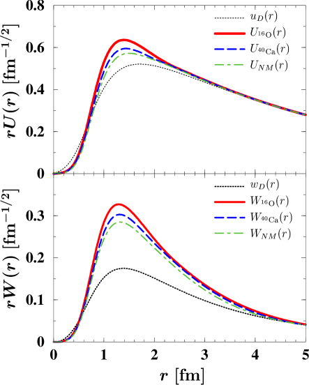
FIG. 1.: Radial components $U(r)$ and $W(r)$ of the AU8^′ QD wave functions in ¹⁶O, ⁴⁰Ca and nuclear matter. Upper panel: the solid and dashed lines show the radial dependence of $U_{A}(r)$ for ¹⁶O and ⁴⁰Ca, respectively. The dot-dashed and dotted lines correspond to the nuclear matter $U_{NM}(r)$ and the bare $u_{D}(r)$. Lower panel: as in the upper panel for the $d$–wave components of the QD and deuteron wave functions.

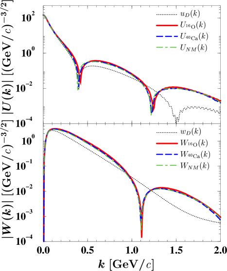
FIG. 2.: As in Fig. 1 in momentum space.

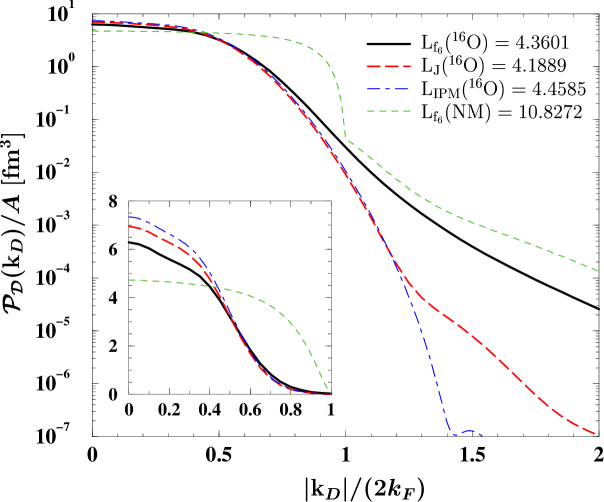
FIG. 3.: Momentum distribution of QD pairs in ¹⁶O as a function of the total momentum $|{{\mathbf{k}}}_{D}|$ (see Eq. (33)). The solid, dashed and dash–dotted lines are the results obtained within the $f_{6}$ and Jastrow correlation models and IPM, respectively. The short–dashed line displays the $f_{6}$ momentum distribution of the QD in nuclear matter at equilibrium density, $\rho_{NM}=0.16~{}\text{fm}^{-3}$. The insert shows a blow up of the region $|{{\mathbf{k}}}_{D}|/(2k_{F})<$ 1, plotted in linear scale. The Levinger factors, ${\textrm{L}}(A)$, for the various calculations are also reported.

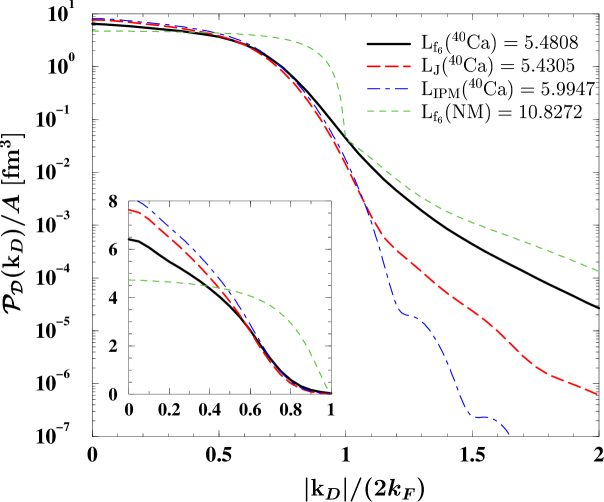
FIG. 4.: As in Fig. 3 for ⁴⁰Ca.

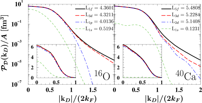
FIG. 5.: Convergence of ${\mathcal{P}_{D}}({{\mathbf{k}}}_{D})/A$ for ¹⁶O and ⁴⁰Ca in the number of natural orbits included in the summation of Eq. (33). The results have been obtained within the $f_{6}$ correlation model.

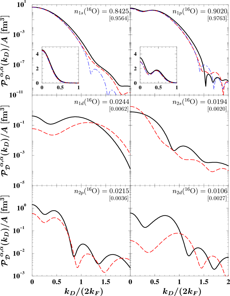
FIG. 6.: Diagonal contributions from the $[1s-2d]$ orbitals to ${\mathcal{P}_{D}}({{\mathbf{k}}}_{D})/A$ for ¹⁶O. The solid, dashed and dash–dotted lines refer to the $f_{6}$, Jastrow and IP models, respectively. The occupation numbers $n_{nl}(^{16}\textrm{O})$ computed with the $f_{6}$ correlation [22] are also reported. The numbers in square brackets refer to the Jastrow case.

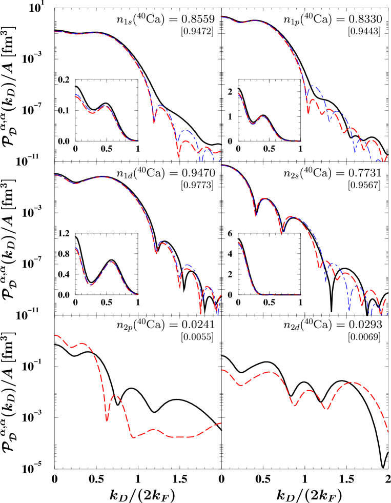
FIG. 7.: As in Fig. 6 for ⁴⁰Ca.

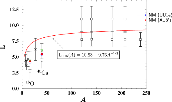
FIG. 8.: Levinger’s factor ${\mathrm{L}}(A)$ for ¹⁶O, ⁴⁰Ca and nuclear matter (shown by the arrows for the UU14 and AU8^′ forces). The filled circles, the empty circles and the triangles show the Levinger’s factors obtained within the $f_{6}$ and Jastrow correlation models and the IPM, respectively. The LDA, as discussed in the text, is also reported (solid line). The phenomenological values of ${\mathrm{L}}_{\text{Lev}}(A)$ corresponding to the photoreaction data of Lepretre et al. [27] (squares) and Ahrens et al. [28] (crosses and diamonds) are taken from Ref. [25]. The empirical values of ${\mathrm{L}}_{\text{Laget}}(A)$, represented by circles in the heavy nuclei region, are from Ref. [26].

REFERENCES

[1]
J. S. Levinger, Phys. Rev. 84(1951)43.
[2]
Yu. K. Khokhlov, J. Exp. Theor. Phys. 23(1952)241.
[3]
K. Gottfried, Nucl. Phys. 5(1958)557.
[4]
O. F. Nemetz, V. G. Neudatchin, A. T. Rudchik,
Yu. F. Smirnov, and Yu. M. Tchuvil’sky,
Nucleon Clustering in Atomic Nuclei and
Multinucleon Transfer Reactions,
(Naukova dumka, Kiev,1988).
[5]
J. S. Levinger, Phys. Lett. B 82(1979)181.
[6]
J. M. Laget, Nucl. Phys. A 358(1981)275c.
[7]
V. G. Kadmenskii, and Yu. L. Ratis,
Sov. J. Nucl. Phys. 33(1981)478.
[8]
A. T. Val’shin, V. G. Kadmenskii, S. G. Kadmenskii,
Yu. L. Ratis, and V. I. Furman,
Sov. J. Nucl. Phys. 33(1981)494.
[9]
O. Benhar, A. Fabrocini, S. Fantoni,
A. Yu. Illarionov, and G. I. Lykasov,
Nucl. Phys. A 703(2002)70.
[10]
I. E. Lagaris, and V. R. Pandharipande,
Nucl. Phys. A 359(1981)331.
[11]
R. B. Wiringa, V. Fiks, and A. Fabrocini,
Phys. Rev. C 38(1988)1010.
[12]
A. Akmal, V. R. Pandharipande, and D. G. Ravenhall,
Phys. Rev. C 58(1998)1804.
[13]
S. Fantoni, and V. R. Pandharipande,
Nucl. Phys. A 427(1984)473.
[14]
O. Benhar, A. Fabrocini, and S. Fantoni,
Nucl. Phys. A 505(1989)267.
[15]
O. Benhar, A. Fabrocini, and S. Fantoni,
Nucl. Phys. A 550(1990)201.
[16]
O. Benhar, A. Fabrocini, S. Fantoni, and I. Sick,
Nucl. Phys. A 579(1994)493.
[17]
O. Benhar, and A. Fabrocini,
Phys. Rev. C 62(2000)034304.
[18]
G. Co’, A. Fabrocini, S. Fantoni, and I. E. Lagaris,
Nucl. Phys. A 549(1992)439.
[19]
G. Co’, A. Fabrocini, and S. Fantoni,
Nucl. Phys. A 568(1994)73.
[20]
A. de Saavedra, G. Co’, A. Fabrocini, and S. Fantoni,
Nucl. Phys. A 605(1996)359.
[21]
A. Fabrocini, A. de Saavedra, and G. Co’,
Phys. Rev. C 61(2000)044302.
[22]
A. Fabrocini, and G. Co’,
Phys. Rev. C 63(2001)044319.
[23]
R. B. Wiringa, V. G. J. Stoks, and R. Schiavilla,
Phys. Rev. C 51(1995)38.
[24]
B. S. Pudliner, V. R. Pandharipande, J. Carlson,
and R. B. Wiringa,
Phys. Rev. Lett. 74(1995)4396;
B. S. Pudliner, V. R. Pandharipande, J. Carlson,
S. C. Pieper, and R. B. Wiringa,
Phys. Rev. C 56(1997)1720.
[25]
M. Anghinolfi, V. Lucherini, N. Bianchi, G. P. Capitani,
P. Corvisiero, E. De Sanctis, P. Di Giacomo, C. Guaraldo,
P. Levi-Sandri, E. Polli, A. R. Reolon, G. Ricco,
M. Sanzone, and M. Taiuti,
Nucl. Phys. A 457(1986)645.
[26]
P. Carlos, H. Beil, R. Bergére, A. Lepretre,
and A. Veyssiére,
Nucl. Phys. A 378(1982)317.
[27]
A. Lepretre, H. Beil, R. Bergére, P. Carlos,
J. Fagot, A. de Miniac, and A. Veyssiére,
Nucl. Phys. A 367(1981)237.
[28]
J. Ahrens, H. Barchert, K. H. Czock, H. B. Eppler,
H. Gimm, H. Gundrum, M. Kroning, P. Rihem,
G. Sita Ram, A. Zieger, and B. Ziegler,
Nucl. Phys. A 251(1975)479.
[29]
V. R. Pandharipande, and R. B. Wiringa,
Rev. Mod. Phys. 51(1979)821.
[30]
A. Fabrocini, A. de Saavedra, G. Co’, and P. Folgarait,
Phys. Rev. C 57(1998)1668.
[31]
S. Fantoni, and A. Fabrocini,
Lecture Notes in Physics: Microscopic Quantum Many-Body
Theories and their Applications,
edited by J. Navarro and A. Polls, 119
(Springer-Verlag, Berlin, 1998).
[32]
A. Fabrocini, and S. Fantoni,
Nucl. Phys. A 503(1989)375.
[33]
A. Fabrocini,
Phys. Lett. B 322(1994)171.
[34]
S. Fantoni,
Advances in Quantum Many-Body Theories:
Introduction to Modern Methods of Quantum Many-Body
Theory and their Applications,
edited by A. Fabrocini, S. Fantoni and E. Krotscheck, 379
(World-Scientific, Singapore, 2002).
[35]
K. E. Schmidt, S. Fantoni, and A. Sarsa,
Quantum Monte Carlo: Recent Advances and Common Problems
in Condensed Matter and Field Theory,
edited by M. Campostrini, M. P. Lombardo, and F. Pederiva, 143
(ETS, Pisa, 2001).
[36]
V. J. G. Stoks, R. A. M. Klomp, M. C. M. Rentmeester,
and J. J. De Swart,
Phys. Rev. C 48(1993)792.
[37]
J. L. Forest, V. R. Pandharipande,
S. C. Pieper, R. B. Wiringa, R. Schiavilla,
and A. Arriaga,
Phys. Rev. C 54(1996)646.
[38]
A. Fabrocini, I. E. Lagaris, M. Viviani, and S. Fantoni,
Phys. Lett. B 156(1985)277.
FIG. 1.:
Radial components and of
the AU8′ QD wave functions
in 16O, 40Ca and nuclear matter.
Upper panel: the solid and dashed lines show the radial dependence of
for 16O and 40Ca, respectively.
The dot-dashed and dotted lines correspond
to the nuclear matter and the bare .
Lower panel: as in the upper panel for the –wave components
of the QD and deuteron wave functions.
FIG. 2.:
As in Fig. 1 in momentum space.
FIG. 3.:
Momentum distribution of QD pairs in 16O as a function of the
total momentum (see Eq. (33)).
The solid, dashed and dash–dotted lines are the results obtained
within the and Jastrow correlation models and IPM, respectively.
The short–dashed line displays
the momentum distribution of the QD in nuclear matter at
equilibrium density, .
The insert shows a blow up of the region 1,
plotted in linear scale. The Levinger factors, ,
for the various calculations are also reported.
FIG. 4.:
As in Fig. 3 for 40Ca.
FIG. 5.:
Convergence of for 16O and 40Ca
in the number of natural orbits included in the summation of
Eq. (33). The results have been obtained within
the correlation model.
FIG. 6.:
Diagonal contributions from the orbitals
to for 16O.
The solid, dashed and dash–dotted lines refer to the ,
Jastrow and IP models, respectively.
The occupation numbers computed with
the correlation [22] are
also reported. The numbers in square brackets refer to the Jastrow case.
FIG. 7.:
As in Fig. 6 for 40Ca.
FIG. 8.:
Levinger’s factor for 16O,
40Ca and nuclear matter (shown by the arrows for the UU14 and
AU8′ forces).
The filled circles, the empty circles and the triangles
show the Levinger’s factors obtained within the and
Jastrow correlation models and the IPM, respectively.
The LDA, as discussed in the text, is also reported (solid line).
The phenomenological values of
corresponding to the photoreaction data of Lepretre et al.
[27] (squares) and Ahrens
et al. [28]
(crosses and diamonds) are taken from
Ref. [25].
The empirical values of ,
represented by circles in the heavy nuclei region,
are from Ref. [26].