Chiral symmetry restoration in linear sigma models with different numbers of quark flavors

Abstract

Chiral symmetry restoration at nonzero temperature is studied in the framework of the $O(4)$ linear sigma model and the $U(N_{f})_{r}\times U(N_{f})_{\ell}$ linear sigma model with $N_{f}=2,\,3$ and 4 quark flavors. We investigate the temperature dependence of the masses of the scalar and pseudoscalar mesons, and the non-strange, strange, and charm condensates within the Hartree approximation as derived from the Cornwall-Jackiw-Tomboulis formalism. We find that the masses of the non-strange and strange mesons at nonzero temperature depend sensitively on the particular symmetry of the model and the number of light quark flavors $N_{f}$. On the other hand, due to the large charm quark mass, neither do charmed mesons significantly affect the properties of the other mesons, nor do their masses change appreciably in the temperature range around the chiral symmetry restoration temperature. In the chiral limit, the transition temperatures for chiral symmetry restoration are surprisingly close to those found in lattice QCD.

I Introduction

For $N_{f}$ massless quark flavors, the QCD Lagrangian has a chiral $U(N_{f})_{r}\times U(N_{f})_{\ell}=SU(N_{f})_{r}\times SU(N_{f})_{\ell}\times U(1)_{V}\times U(1)_{A}$ symmetry. Here, $V=r+\ell$, while $A=r-\ell$. The $U(1)_{V}$ symmetry corresponds to baryon number conservation. It is always respected and thus plays no role in the symmetry breaking patterns considered in the following. In the vacuum, a non-vanishing expectation value of the quark condensate, $\langle\bar{q}_{\ell}\,q_{r}\rangle\neq 0$, spontaneously breaks the above symmetry to $SU(N_{f})_{V}$. This gives rise to $N_{f}^{2}$ Goldstone bosons which dominate the low-energy dynamics of the theory. As shown by ’t Hooft ’t Hooft (1976a, b), instantons break the $U(1)_{A}$ symmetry explicitly to $Z(N_{f})_{A}$ Pisarski and Wilczek (1984). (For the low-energy dynamics of QCD, however, this discrete symmetry is irrelevant.) Consequently, one of the $N_{f}^{2}$ Goldstone bosons becomes massive, leaving $N_{f}^{2}-1$ Goldstone bosons. The $SU(N_{f})_{r}\times SU(N_{f})_{\ell}\times U(1)_{A}$ symmetry of the QCD Lagrangian is also explicitly broken by nonzero quark masses. The $N_{f}^{2}-1$ low-energy degrees of freedom then become pseudo-Goldstone bosons. For $M\leq N_{f}$ degenerate quark flavors, an $SU(M)_{V}$ symmetry is preserved.

As indicated by lattice QCD calculations Karsch (2002), chiral symmetry is restored at temperatures around $\sim 150$ MeV (at zero net-baryon number density). It is difficult to determine the order of the chiral phase transition on the lattice. At this time, lattice calculations have not unambiguously answered this question. For physical values of the quark masses, calculations with staggered fermions Brown et al. (1990) favor a smooth crossover transition, while calculations with Wilson fermions Iwasaki et al. (1996) predict the transition to be of first order.

For vanishing quark masses, i.e., in the chiral limit, however, one can use universality arguments to determine the order of the phase transition. According to universality, the order of the chiral transition in QCD is identical to that in a theory with the same chiral symmetries as QCD, for instance, the $U(N_{f})_{r}\times U(N_{f})_{\ell}$ linear sigma model. This argument was employed by Pisarski and Wilczek Pisarski and Wilczek (1984) who found that for $N_{f}=2$ flavors of massless quarks, the transition can be of second order, if the $U(1)_{A}$ symmetry is explicitly broken by instantons. It is driven first order by fluctuations, if the $U(1)_{A}$ symmetry is restored at $T_{c}$. For $N_{f}=3$ massless flavors, the transition is always first order. In this case, the term which breaks the $U(1)_{A}$ symmetry explicitly is a cubic invariant, and consequently drives the transition first order. In the absence of explicit $U(1)_{A}$ symmetry breaking, the transition is fluctuation-induced of first order. For $N_{f}=4$, the same argument leads to a first order chiral transition in the absence of the $U(1)_{A}$ anomaly. The term which breaks the $U(1)_{A}$ symmetry is no longer a cubic invariant, but of quartic order in the fields. Since this term does not generate an infrared-stable fix point, the transition remains of first order.

For nonzero quark masses, the chiral symmetry of QCD is explicitly broken. Nonzero quark masses act like a magnetic field in spin systems, such that a second order phase transition becomes a crossover transition. When the quark masses increase, a first order phase transition may for a while remain of first order, but it will ultimately become a crossover transition, too. In order to decide whether this happens for a particular choice of quark masses, universality arguments cannot be applied and one has to resort to numerical calculations. As an alternative to lattice QCD calculations, one can also use linear sigma models to investigate this question Lenaghan (2001).

Studying the linear sigma model at nonzero temperature, however, requires many-body resummation schemes, because infrared divergences cause naive perturbation theory to break down Dolan and Jackiw (1974). In these resummation schemes, one necessarily has to make approximations by selecting certain subsets of diagrams. The most commonly employed scheme is the Hartree approximation. This approximation fails to reproduce the correct order of the chiral transition for the $O(4)$ linear sigma model: the transition is of second order, while the Hartree approximation yields a first order transition. For $U(N_{f})_{r}\times U(N_{f})_{\ell}$ linear sigma models with $N_{f}=3$, however, the Hartree approximation correctly produces a first order chiral transition Lenaghan et al. (2000). For $N_{f}=2$, in the absence of the $U(1)_{A}$ anomaly the transition is of first order and, as will be shown in this paper, the Hartree approximation agrees with this result. With the $U(1)_{A}$ anomaly, the transition is of second order. We shall find that the Hartree approximation (slightly) violates this prediction by producing a (weak) first order transition.

The utility of linear sigma models, however, transcends further than just predicting the order of the chiral phase transition. The degrees of freedom of the $U(N_{f})_{r}\times U(N_{f})_{\ell}$ linear sigma model are the scalar and pseudoscalar mesons. In the vacuum, the latter are the (pseudo-) Goldstone bosons of chiral symmetry breaking. Thus, the linear sigma model can also be viewed as an effective low-energy theory for QCD. At high temperatures, chiral symmetry is restored. Consequently, chiral partners among the scalar and pseudoscalar mesons must become degenerate in mass. Since the $U(N_{f})_{r}\times U(N_{f})_{\ell}$ linear sigma model treats both scalar and pseudoscalar mesons on the same footing, it is particularly suited to describe the change of meson properties across the chiral transition. Note that, in the case of a first order chiral transition which coincides with the deconfinement transition, the correct degrees of freedom in the high-temperature phase are quark and gluons instead of mesons. However, in the case of a crossover transition mesonic degrees of freedom are well-defined even above the chiral transition temperature.

	$O(4)$	$U(2)_{r}\times U(2)_{\ell}$	$U(3)_{r}\times U(3)_{\ell}$	$U(4)_{r}\times U(4)_{\ell}$
Explicit chiral
symmetry breaking	$\surd$	$\surd$	$\surd$	$\surd$
with $U(1)_{A}$
anomaly
Explicit chiral
symmetry breaking	$\times$	$\surd$	$\surd$	$-$
without $U(1)_{A}$
anomaly
Chiral limit
with $U(1)_{A}$	$\surd$	$\surd$	$\surd$	$-$
anomaly
Chiral limit
without $U(1)_{A}$	$\times$	$\surd$	$\surd$	$-$
anomaly

Table 1: The table shows the symmetry breaking patterns studied in this paper. The $\surd$ symbol indicates that the specific symmetry breaking pattern is physically interesting and investigated here. The $\times$ symbol indicates that this symmetry breaking pattern does not exist at all and the $-$ symbolizes that the respective symmetry breaking pattern is not studied.

In the present work, we follow this line of arguments and investigate the change of meson masses and quark condensates with temperature in the framework of $U(N_{f})_{r}\times U(N_{f})_{\ell}$ linear sigma models. We focus in particular on the question how the number of quark flavors $N_{f}$ changes the temperature dependence of the meson masses and the quark condensates. For a given $N_{f}$, we furthermore investigate the different patterns of symmetry breaking arising from the presence or absence of the $U(1)_{A}$ anomaly, and from taking zero or nonzero values for the quark masses. In this sense, the present study is an extension of previous work Lenaghan and Rischke (2000); Lenaghan et al. (2000). Table 1 presents an overview of the different models and patterns of symmetry breaking studied in this paper.

The $U(2)_{r}\times U(2)_{\ell}$ linear sigma model has eight degrees of freedom: the scalar fields are the $\sigma$ meson and the three $a_{0}$ mesons, the pseudoscalar fields are the $\eta$ meson and the three pions. With spontaneous breaking of the $U(2)_{A}$ chiral symmetry, but without the $U(1)_{A}$ anomaly, the pions and the $\eta$ meson are (pseudo-) Goldstone bosons, while the $\sigma$ and $a_{0}$ meson are heavy states. With the $U(1)_{A}$ anomaly, the $\eta$ meson also becomes heavy.

With explicit breaking of the $U(1)_{A}$ symmetry due to the anomaly (and neglecting the $U(1)_{V}$ symmetry of baryon number conservation), the remaining symmetry of the $U(2)_{r}\times U(2)_{\ell}$ linear sigma model is $SU(2)_{r}\times SU(2)_{\ell}$. This group is isomorphic to $O(4)$. The appropriate effective theory incorporating this symmetry is the $O(4)$ linear sigma model Gell-Mann and Levy (1960). This model has only four degrees of freedom, the $\sigma$ meson and the three pions. In this sense, it represents the limit of the $U(2)_{r}\times U(2)_{\ell}$ model for maximum $U(1)_{A}$ symmetry breaking. The $U(2)_{r}\times U(2)_{\ell}$ model is more general, since it allows to consider the properties of mesons also without the $U(1)_{A}$ anomaly.

In the limit of maximum $U(1)_{A}$ symmetry breaking, the $\eta$ and $a_{0}$ mesons become infinitely heavy and are thus removed from the spectrum of physical excitations. This approximation is justified at small temperatures, where the dynamics is determined by the lightest hadronic degrees of freedom, i.e., the pions and, to some extent, the $\sigma$ meson. At higher temperatures and, in particular, around the chiral transition, however, heavier mesons become more and more important. It is therefore interesting to compare the results of the $O(4)$ model with those of the $U(2)_{r}\times U(2)_{\ell}$ model which incorporates these heavier degrees of freedom. Note that the $O(4)$ linear sigma model at nonzero temperature has been discussed in Refs. Petropoulos (1999); Lenaghan and Rischke (2000).

In the physical hadron spectrum, the kaons are lighter than the $a_{0}$ and $\eta$ mesons and thus are more copiously produced at nonzero temperature. Consequently, the kaons are expected to influence the dynamics of the system to a larger extent than the $a_{0}$ and $\eta$ mesons. Therefore, the $U(2)_{r}\times U(2)_{\ell}$ model is unrealistic in the sense that it neglects these strange meson degrees of freedom. From a physical point of view, it is thus necessary to enlarge the symmetry group to $U(3)_{r}\times U(3)_{\ell}$ and study the corresponding linear sigma model. Nevertheless, it is still interesting to compare the $U(2)_{r}\times U(2)_{\ell}$ model with the $U(3)_{r}\times U(3)_{\ell}$ model in order to see how the strange degrees of freedom affect the results. The $U(3)_{r}\times U(3)_{\ell}$ model was previously studied at nonzero temperature in Ref. Lenaghan et al. (2000).

Finally, we extend our investigations by including the charm degree of freedom. In principle, the corresponding linear sigma model has an $SU(4)_{r}\times SU(4)_{\ell}\times U(1)_{A}$ symmetry, but in nature this symmetry is strongly explicitly broken by the large charm quark mass. Therefore, we only consider the physically relevant case of explicit chiral symmetry breaking with $U(1)_{A}$ anomaly.

For all cases considered (see Table 1) we study the meson masses and the condensates as functions of temperature. In the chiral limit, we determine the phase transition temperatures by computing the effective potentials. In this aspect, we extend the previous study of Ref. Lenaghan et al. (2000). For the $O(4)$ model, this has already been done in Ref. Petropoulos (1999).

Our calculations are done in the Hartree approximation which we derive within the Cornwall-Jackiw-Tomboulis (CJT) formalism Cornwall et al. (1974). The Hartree approximation has the advantage that the meson self-energies become independent of momentum and energy and one only has to solve gap equations for the meson masses as a function of temperature. To go beyond the Hartree approximation, for instance by including energy-momentum dependent contributions to the self-energies, is considerably more difficult van Hees and Knoll (2000, 2002); Van Hees and Knoll (2002); van Hees and Knoll (2002), and will be deferred to a future publication.

The remainder of this paper is organized as follows. In Sec. II, we review the formulas of the CJT formalism, which are relevant for the present study, and apply them to the $O(4)$ model and the $U(N_{f})_{r}\times U(N_{f})_{\ell}$ linear sigma models for $N_{f}=2,3,$ and 4. In Sec. III, it is shown how to determine the coupling constants of the different models from the vacuum properties of the mesons and condensates. In Sec. IV, we discuss the temperature dependence of the masses and the condensates. We conclude this work in Sec. V with a summary of our results.

We use the imaginary-time formalism to compute quantities at nonzero temperature. Our notation is

$$\int_{k}\,f(k)\equiv T\sum_{n=-\infty}^{\infty}\int\frac{d^{3}{\bf k}}{(2\pi)^{3}}\,f(2\pi inT,{\bf k})\,\,\,\,,\,\,\,\,\int_{x}\,f(x)\equiv\int^{1/T}_{0}d\tau\int d^{3}{\bf x}\,f(\tau,{\bf x})\,\,.$$ (1)

Our units are $\hbar=c=k_{B}=1$. The metric tensor is $g^{\mu\nu}={\rm diag}(+,-,-,-)$. Throughout this work, all latin subscripts are adjoint $U(N_{f})$ indices, $a=0,\ldots,N_{f}^{2}-1$, and a summation over repeated indices is understood.

II Linear Sigma Models in the Hartree approximation

II.1 The CJT formalism

The CJT formalism Cornwall et al. (1974) generalizes the concept of the effective action for one-point functions to that of an effective action for one- and two-point functions. It is particularly useful for theories with spontaneously broken symmetry. In this case, truncating the standard loop expansion for the effective action Jackiw (1974) at some given order, at nonzero temperature one may obtain unphysical, tachyonic propagation of quasiparticles with small momenta. The reason for this failure of the standard loop expansion is that only the expectation value of the one-point function is self-consistently determined in this approach. The CJT formalism goes beyond the standard loop expansion by self-consistently determining the expectation value for the two-point function in addition to that of the one-point function. Effectively, this amounts to solving a Dyson-Schwinger equation for the two-point functions and yields a self-consistent computation of the quasiparticle self-energy. For translationally invariant systems, the effective action becomes the effective potential. To give an example, consider the general Lagrangian

$${\cal L}(\varphi)=\frac{1}{2}\,\partial_{\mu}\varphi\,\partial^{\mu}\varphi-U(\varphi)$$ (2)

for a scalar quantum field $\varphi$. The effective potential in the CJT formalism reads

$$V[\bar{\phi},\bar{G}]=U(\bar{\phi})+\frac{1}{2}\int_{k}\,\ln\bar{G}^{-1}(k)+\frac{1}{2}\,\int_{k}\,\left[G^{-1}(k;\bar{\phi})\,\bar{G}(k)-1\right]+V_{2}[\bar{\phi},\bar{G}]\,\,,$$ (3)

where $\bar{\phi}$ is a $c$-number field (it is the expectation value of the quantum field $\varphi$ in the presence of an external source), $U(\bar{\phi})$ is the classical potential energy density (the tree-level potential) in the Lagrangian (2), and $G^{-1}$ is the inverse of the tree-level propagator,

$$G^{-1}(k;\bar{\phi})\equiv-k^{2}+U^{\prime\prime}(\bar{\phi})\,\,.$$ (4)

Here, $U^{\prime\prime}(\bar{\phi})$ is the second derivative of $U(\bar{\phi})$ with respect to $\bar{\phi}$. The last term in Eq. (3), $V_{2}[\bar{\phi},\bar{G}]$, is the sum of all two-particle irreducible vacuum diagrams where all lines represent full propagators $\bar{G}$. The expectation values of the one-point function, $\phi$, and of the two-point function, ${\cal G}(k)$ are determined from the stationarity conditions

$$\left.\frac{\delta V[\bar{\phi},\bar{G}]}{\delta\bar{\phi}}\,\right|_{\bar{\phi}=\phi,\,\bar{G}={\cal G}}=0\,\,,$$ (5a)

$$\left.\frac{\delta V[\bar{\phi},\bar{G}]}{\delta\bar{G}(k)}\,\right|_{\bar{\phi}=\phi,\,\bar{G}={\cal G}}=0\,\,.$$ (5b)

With Eq. (3), the latter can be written in the form

$${\cal G}^{-1}(k)=G^{-1}(k;\phi)+\Pi(k)\,\,,$$ (6a)

where

$$\Pi(k)\equiv 2\left.\frac{\delta V_{2}[\bar{\phi},\bar{G}]}{\delta\bar{G}(k)}\right|_{\bar{\phi}=\phi,\,\bar{G}={\cal G}}$$ (6b)

is the self-energy. Since $\Pi(k)$ is in general a functional of ${\cal G}$, Eq. (6a) represents a Schwinger-Dyson equation for the full (dressed) propagator.

The standard effective potential for the expectation value of the one-point function, $V(\bar{\phi})$, is obtained from the effective potential (3) by taking the full propagator $\bar{G}$ to be a function of $\bar{\phi}$, instead of an independent variable,

$$V(\bar{\phi})=V[\bar{\phi},\hat{G}(\bar{\phi})]\,\,,$$ (7)

where $\hat{G}(k;\bar{\phi})$ is determined from

$$\left.\frac{\delta V[\bar{\phi},\bar{G}]}{\delta\bar{G}(k)}\,\right|_{\bar{G}=\hat{G}}=0\,\,,$$ (8)

which is equivalent to

$$\hat{G}^{-1}(k;\bar{\phi})=G^{-1}(k;\bar{\phi})+\hat{\Pi}(k;\bar{\phi})\,\,,$$ (9a)

where

$$\hat{\Pi}(k;\bar{\phi})\equiv 2\left.\frac{\delta V_{2}[\bar{\phi},\bar{G}]}{\delta\bar{G}(k)}\right|_{\bar{G}=\hat{G}}.$$ (9b)

This expression and Eq. (3) can be used to obtain a compact form of the standard effective potential

$$V(\bar{\phi})=U(\bar{\phi})+\frac{1}{2}\int_{k}\,\ln\hat{G}^{-1}(k;\bar{\phi})-\,\frac{1}{2}\int_{k}\,\hat{\Pi}(k;\bar{\phi})\,\hat{G}(k;\bar{\phi})+V_{2}[\bar{\phi},\hat{G}]\,\,.$$ (10)

Since $V_{2}$ contains infinitely many diagrams, an exact calculation is impossible. In practice, one has to restrict the computation of $V_{2}$ to a finite number of diagrams. The selected set of diagrams defines a particular many-body approximation. Cutting internal lines in these diagrams according to Eq. (6b), one obtains the diagrams contributing to the self-energy of the quasiparticles in this approximation scheme. Solving the Dyson-Schwinger equation (6a) provides a self-consistent calculation of this self-energy. In general, the Dyson-Schwinger equation is an integral equation for the self-energy as a function of energy and momentum.

If one only takes the double-bubble diagrams on the left-hand side of Fig. 1 into account in the calculation of $V_{2}$, one obtains the Hartree approximation. Cutting these diagrams yields the well-known tadpole diagrams for the self-energy, cf. the right-hand side of Fig. 1. The Dyson-Schwinger equation (6a) is a self-consistency equation for this self-energy due to the fact that the internal lines in the tadpole diagrams represent full propagators. The Hartree approximation is a particularly simple many-body approximation scheme, because the tadpole diagrams are independent of energy and momentum, and thus the Dyson-Schwinger equations are no longer integral equations, but become fix-point equations for the quasiparticle masses.

Figure 1: Left-hand side: the double-bubble diagrams. Full lines are scalar particles, dashed lines are pseudoscalar particles. Right-hand side: the tadpole contributions to the self-energies obtained by cutting a line in the double-bubble diagrams on the left-hand side.

II.2 The $O(4)$ model

In this subsection, we apply the CJT formalism to the $O(N)$ model. Our numerical results presented in Sec. IV are exclusively for the case $N=4$. The CJT effective potential for the $O(N)$ model is Lenaghan and Rischke (2000)

$$V[\bar{\sigma},\bar{S},\bar{P}] = U(\bar{\sigma})+\frac{1}{2}\int_{k}\left[\,\ln\bar{S}^{-1}(k)+S^{-1}(k;\bar{\sigma})\,\bar{S}(k)-1\,\right]$$ (11)

$$+ \frac{N-1}{2}\int_{k}\,\left[\,\ln\bar{P}^{-1}(k)+P^{-1}(k;\bar{\sigma})\,\bar{P}(k)-1\,\right]+V_{2}[\bar{\sigma},\bar{S},\bar{P}]\,\,,$$

where $\bar{\sigma}$ is the expectation value of the scalar field (in the presence of external sources). Because the vacuum of QCD has even parity, the expectation values of the pseudoscalar fields can be set to zero. The quantities $\bar{S}$ and $\bar{P}$ are the full propagators for scalar and pseudoscalar particles, while $S^{-1}$ and $P^{-1}$ are the corresponding inverse tree-level propagators,

$$S^{-1}(k;\bar{\sigma}) = -k^{2}+m_{\sigma}^{2}(\bar{\sigma})\,\,,$$ (12a)

$$P^{-1}(k;\bar{\sigma}) = -k^{2}+m_{\pi}^{2}(\bar{\sigma})\,\,,$$ (12b)

where the tree-level masses are

$$m_{\sigma}^{2}(\bar{\sigma}) = \mu^{2}+\frac{12\,\lambda}{N}\,\bar{\sigma}^{2}\,\,,$$ (13a)

$$m_{\pi}^{2}(\bar{\sigma}) = \mu^{2}+\frac{4\,\lambda}{N}\,\bar{\sigma}^{2}\,\,.$$ (13b)

The constant $\mu^{2}$ is the bare mass term in the Lagrangian of the $O(N)$ model, while $\lambda$ is the four-point coupling constant. For $\mu^{2}<0$, the $O(N)$ symmetry is spontaneously broken to $O(N-1)$, leading to $N-1$ Goldstone bosons. The tree-level potential is

$$U(\bar{\sigma})=\frac{1}{2}\,\mu^{2}\,\bar{\sigma}^{2}+\frac{\lambda}{N}\,\bar{\sigma}^{4}-H\,\bar{\sigma}\,\,,$$ (14)

where $H$ is a term which breaks the $O(N)$ symmetry explicitly to $O(N-1)$. $V_{2}[\bar{\sigma},\bar{S},\bar{P}]$ is the sum of all two-particle irreducible diagrams. In the following, we restrict ourselves to the Hartree approximation, i.e., we take into account only the double-bubble diagrams shown on the left-hand side of Fig. 1. These diagrams have no explicit $\bar{\sigma}$ dependence. Then, only tadpole diagrams (with resummed propagators) contribute to the self-energies, cf. the right-hand side of Fig. 1. In the Hartree approximation,

$$V_{2}[\bar{S},\bar{P}] = 3\,\frac{\lambda}{N}\left[\int_{k}\,\bar{S}(k)\right]^{2}+(N+1)(N-1)\,\frac{\lambda}{N}\left[\int_{k}\,\bar{P}(k)\right]^{2}$$ (15)

$$+ 2\,(N-1)\frac{\lambda}{N}\left[\int_{k}\,\bar{S}(k)\right]\left[\int_{p}\,\bar{P}(p)\right]\,\,.$$

The stationarity conditions (5a) and (5b) read

$$H = \mu^{2}\,\sigma+\frac{4\lambda}{N}\,\sigma^{3}+\frac{4\lambda}{N}\,\sigma\int_{q}\,\left[3\,{\cal S}(q)+(N-1)\,{\cal P}(q)\right]\,\,,$$ (16a)

$${\cal S}^{-1}(k) = -k^{2}+M_{\sigma}^{2}\,\,,$$ (16b)

$${\cal P}^{-1}(k) = -k^{2}+M_{\pi}^{2}\,\,,$$ (16c)

where ${M}_{\sigma}$ and ${M}_{\pi}$ are the $\sigma$ and pion masses dressed by contributions from the diagrams of Fig. 1,

$$M_{\sigma}^{2} = m_{\sigma}^{2}(\sigma)+\frac{4\lambda}{N}\left[3\,\int_{q}\,{\cal S}(q)+(N-1)\,\int_{q}\,{\cal P}(q)\right]$$ (17a)

$$M_{\pi}^{2} = m_{\pi}^{2}(\sigma)+\frac{4\lambda}{N}\left[\int_{q}\,{\cal S}(q)+(N+1)\,\int_{q}\,{\cal P}(q)\right]\,\,.$$ (17b)

Using Eqs. (17a) and (17b), Eq. (16a) can be written in the compact form:

$$H=\sigma\left[M_{\sigma}^{2}-\frac{8\lambda}{N}\,\sigma^{2}\right]\,\,.$$ (17c)

Equations (17a), (17b), and (17c) are the stationarity conditions of the $O(N)$ model in the Hartree approximation. The explicit calculation of the tadpole integrals $\int_{q}{\cal S}(q)$ and $\int_{q}{\cal P}(q)$ will be discussed in Sec. II.4.

II.3 The $U(N_{f})_{r}\times U(N_{f})_{\ell}$ linear sigma model for $N_{f}=2,\,3$ and $4$ flavors

The application of the CJT formalism to the $U(N_{f})_{r}\times U(N_{f})_{\ell}$ linear sigma model for $N_{f}=3$ was discussed in Ref. Lenaghan et al. (2000). Since we want to treat the cases $N_{f}=2$ and $N_{f}=4$ on the same footing, we derive the CJT effective potential in somewhat greater detail than in the last subsection.

The Lagrangian of the $U(N_{f})_{r}\times U(N_{f})_{\ell}$ linear sigma model for $N_{f}=2,\,3$ or 4 flavors is given by Levy (1967); Hu (1974); Schechter and Singer (1975); Geddes (1980)

$${\cal L}(\Phi) = {\rm Tr}\left(\partial_{\mu}\Phi^{\dagger}\partial^{\mu}\Phi-m^{2}\,\Phi^{\dagger}\Phi\right)-\lambda_{1}\left[{\rm Tr}\left(\Phi^{\dagger}\Phi\right)\right]^{2}-\lambda_{2}{\rm Tr}\left(\Phi^{\dagger}\Phi\right)^{2}$$ (18)

$$+ c\,\left[{\rm det}\left(\Phi\right)+{\rm det}\left(\Phi^{\dagger}\right)\right]+{\rm Tr}\left[H\left(\Phi+\Phi^{\dagger}\right)\right]\,\,.$$

$\Phi$ is a complex $N_{f}\times N_{f}$ matrix parametrizing the scalar and pseudoscalar mesons,

$$\Phi=T_{a}\,\phi_{a}=T_{a}\,(\sigma_{a}+i\pi_{a})\,\,,$$ (19a)

where $$\sigma_{a} J^{\rm P}=0^{+} \pi_{a} J^{\rm P}=0^{-} N_{f}\times N_{f} H$$ are the scalar () fields and are the pseudoscalar () fields. The matrix breaks the symmetry explicitly and is chosen as

$$H=T_{a}\,h_{a}\,\,,$$ (19b)

where $h_{a}$ are external fields. $T_{a}$ are the generators of $U(N_{f})$. The $T_{a}$ are normalized such that ${\rm Tr}(T_{a}T_{b})=\delta_{ab}/2$. They obey the $U(N_{f})$ algebra with

$$\left[T_{a},T_{b}\right] = i\,f_{abc}\,T_{c}\,\,,$$ (20a)

$$\left\{T_{a},T_{b}\right\} = d_{abc}\,T_{c}\,\,,$$ (20b)

where $$f_{abc} d_{abc} SU(N_{f}) a,b,c=1,\ldots,N_{f}^{2}-1$$ and are the standard antisymmetric and symmetric structure constants of , , and

$$f_{ab0}\equiv 0\,\,\,\,,\,\,\,\,d_{ab0}\equiv\sqrt{\frac{2}{N_{f}}}\,\delta_{ab}\,\,.$$ (20c)

The terms in the first line of Eq. (18) are invariant under $U(N_{f})_{r}\times U(N_{f})_{\ell}\cong U(N_{f})_{V}\times U(N_{f})_{A}$ transformations. The determinant terms are invariant under $SU(N_{f})_{r}\times SU(N_{f})_{\ell}\cong SU(N_{f})_{V}\times SU(N_{f})_{A}$, but break the $U(1)_{A}$ symmetry explicitly. These terms arise from the $U(1)_{A}$ anomaly of the QCD vacuum. The last term in Eq. (18) breaks the axial and possibly the $SU(N_{f})_{V}$ vector symmetries explicitly.

In the following we discuss the three different cases $N_{f}=2,\,3,$ and 4 in detail. The identification of the $\sigma_{a}$ and $\pi_{a}$ fields with the physical scalar and pseudoscalar mesons is given in Appendix A.

A non-vanishing vacuum expectation value for $\Phi$,

$$\langle\Phi\rangle\equiv T_{a}\,\bar{\sigma}_{a}\,\,,$$ (21)

breaks the chiral symmetry spontaneously. (If the vacuum does not break parity, the fields $\pi_{a}$ cannot assume a non-vanishing vacuum expectation value.) Shifting the $\Phi$ field by this expectation value, the Lagrangian can be rewritten as

$${\cal L} = \frac{1}{2}\left[\partial_{\mu}\sigma_{a}\partial^{\mu}\sigma_{a}+\partial_{\mu}\pi_{a}\partial^{\mu}\pi_{a}-\sigma_{a}(m_{S}^{2})_{ab}\sigma_{b}-\pi_{a}(m_{P}^{2})_{ab}\pi_{b}\right]$$ (22)

$$- \,\left[\,\frac{4}{3}\,{\cal F}_{abcd}\,\bar{\sigma}_{d}-\delta(N_{f},3)\,{\cal G}_{abc}+\frac{4}{3}\,\delta(N_{f},4)\,{\cal G}_{abcd}\,\bar{\sigma}_{d}\,\right]\,\sigma_{a}\sigma_{b}\sigma_{c}$$

$$- \,\left[\frac{}{}4\,{\cal H}_{abcd}\,\bar{\sigma}_{d}+3\,\delta(N_{f},3)\,{\cal G}_{abc}-4\,\delta(N_{f},4)\,{\cal G}_{abcd}\,\bar{\sigma}_{d}\,\right]\,\pi_{a}\pi_{b}\sigma_{c}$$

$$- 2\left[\frac{}{}{\cal H}_{abcd}-\delta(N_{f},4)\,{\cal G}_{abcd}\,\right]\,\sigma_{a}\sigma_{b}\pi_{c}\pi_{d}$$

$$- \frac{1}{3}\,\left[\frac{}{}{\cal F}_{abcd}+\delta(N_{f},4)\,{\cal G}_{abcd}\,\right]\,(\sigma_{a}\sigma_{b}\sigma_{c}\sigma_{d}+\pi_{a}\pi_{b}\pi_{c}\pi_{d})$$

$$- U(\bar{\sigma})\,\,,$$

where $\delta(n,m)\equiv\delta_{nm}$ is the Kronecker delta and the fields $\sigma_{a}$ and $\pi_{a}$ are the fluctuations around the expectation values $\bar{\sigma}_{a}$. The latter are determined from the condition $dU(\bar{\sigma})/d\bar{\sigma}_{a}=0$. The tree-level potential is

$$U(\bar{\sigma}) = \frac{m^{2}}{2}\,\bar{\sigma}_{a}^{2}-\left[\frac{}{}3\,\delta(N_{f},2)\,{\cal G}_{ab}+\delta(N_{f},3)\,{\cal G}_{abc}\,\bar{\sigma}_{c}\,\right]\bar{\sigma}_{a}\bar{\sigma}_{b}$$ (23)

$$+ \frac{1}{3}\left[\frac{}{}{\cal F}_{abcd}+\delta(N_{f},4)\,{\cal G}_{abcd}\,\right]\,\bar{\sigma}_{a}\bar{\sigma}_{b}\bar{\sigma}_{c}\bar{\sigma}_{d}-h_{a}\,\bar{\sigma}_{a}\,\,.$$

The coefficients ${\cal F}_{abcd}$, ${\cal G}_{ab}$, ${\cal G}_{abc}$, ${\cal G}_{abcd}$, and ${\cal H}_{abcd}$ are given by

$${\cal F}_{abcd} = \frac{\lambda_{1}}{4}\,\left(\delta_{ab}\delta_{cd}+\delta_{ad}\delta_{bc}+\delta_{ac}\delta_{bd}\right)+\frac{\lambda_{2}}{8}\,\left(d_{abn}d_{ncd}+d_{adn}d_{nbc}+d_{acn}d_{nbd}\right)\,\,,$$ (24a)

$${\cal G}_{ab} = \frac{c}{6}\left[\frac{}{}\delta_{a0}\delta_{b0}-\delta_{a1}\delta_{b1}-\delta_{a2}\delta_{b2}-\delta_{a3}\delta_{b3}\;\right]\,\,,$$ (24b)

$${\cal G}_{abc} = \frac{c}{6}\left[d_{abc}-\frac{3}{2}\,(\delta_{a0}d_{0bc}+\delta_{b0}d_{a0c}+\delta_{c0}d_{ab0})+\frac{9}{2}\,d_{000}\delta_{a0}\delta_{b0}\delta_{c0}\right]\,\,,$$ (24c)

$${\cal G}_{abcd} = -\frac{c}{16}\,\left[\frac{}{}\delta_{ab}\delta_{cd}+\delta_{ad}\delta_{bc}+\delta_{ac}\delta_{bd}-\left(d_{abn}d_{ncd}+d_{adn}d_{nbc}+d_{acn}d_{nbd}\right)+16\,\delta_{a0}\delta_{b0}\delta_{c0}\delta_{d0}\right.$$ (24d)

$$\hskip 14.22636pt-\;4\left(\delta_{a0}\delta_{b0}\delta_{cd}+\delta_{a0}\delta_{c0}\delta_{bd}+\delta_{a0}\delta_{d0}\delta_{bc}+\delta_{b0}\delta_{c0}\delta_{ad}+\delta_{b0}\delta_{d0}\delta_{ac}+\delta_{d0}\delta_{c0}\delta_{ab}\right)$$

$$\hskip 14.22636pt+\;\sqrt{8}\left.\left(\delta_{a0}d_{bcd}+\delta_{b0}d_{cda}+\delta_{c0}d_{dab}+\delta_{d0}d_{abc}\right)\frac{}{}\right]\,\,,$$

$${\cal H}_{abcd} = \frac{\lambda_{1}}{4}\,\delta_{ab}\delta_{cd}+\frac{\lambda_{2}}{8}\,\left(d_{abn}d_{ncd}+f_{acn}f_{nbd}+f_{bcn}f_{nad}\right)\,\,.$$ (24e)

The tree-level masses, $[m_{S}^{2}]_{ab}$ and $[m_{P}^{2}]_{ab}$, are given by

$$\left[m_{S}^{2}(\bar{\sigma})\right]_{ab} = m^{2}\delta_{ab}-6\left[\delta(N_{f},2)\,{\cal G}_{ab}+\delta(N_{f},3){\cal G}_{abc}\bar{\sigma}_{c}\right]+4\left[{\cal F}_{abcd}+\delta(N_{f},4){\cal G}_{abcd}\right]\,\bar{\sigma}_{c}\bar{\sigma}_{d}\,,$$ (25a)

$$\left[m_{P}^{2}(\bar{\sigma})\right]_{ab} = m^{2}\delta_{ab}+6\left[\delta(N_{f},2)\,{\cal G}_{ab}+\delta(N_{f},3){\cal G}_{abc}\bar{\sigma}_{c}\right]+4\left[{\cal H}_{abcd}-\delta(N_{f},4){\cal G}_{abcd}\right]\,\bar{\sigma}_{c}\bar{\sigma}_{d}\,.$$ (25b)

In general, these mass matrices are not diagonal. Consequently, the fields ($\sigma_{a}$, $\pi_{a}$) in the standard basis of $U(N_{f})$ generators are not mass eigenstates. Since the mass matrices are symmetric and real, diagonalization is achieved by an orthogonal transformation,

$$\tilde{\sigma}_{i} = O^{(S)}_{ia}\,\sigma_{a}\,\,,$$ (26a)

$$\tilde{\pi}_{i} = O^{(P)}_{ia}\,\pi_{a}\,\,,$$ (26b)

$$\left[\tilde{m}_{S,P}^{2}\right]_{i} = O^{(S,P)}_{ai}\,\left[m_{S,P}^{2}\right]_{ab}\,O^{(S,P)}_{bi}\,\,.$$ (26c)

The effective potential of the $U(N_{f})_{r}\times U(N_{f})_{\ell}$ linear sigma model in the CJT formalism reads

$$V[\bar{\sigma},\bar{S},\bar{P}] = U(\bar{\sigma})+\frac{1}{2}\int_{k}\,\left\{\left[\ln\bar{S}^{-1}(k)\right]_{aa}+\left[\ln\bar{P}^{-1}(k)\right]_{aa}\right\}$$ (27)

$$+ \frac{1}{2}\,\int_{k}\,\left[S^{-1}_{ab}(k;\bar{\sigma})\,\bar{S}_{ba}(k)+P^{-1}_{ab}(k;\bar{\sigma})\,\bar{P}_{ba}(k)-2\delta_{ab}\,\delta_{ba}\right]+V_{2}[\bar{\sigma},\bar{S},\bar{P}]\,\,.$$

Here, $U(\bar{\sigma})$ is the tree-level potential of Eq. (23), and

$$S_{ab}^{-1}(k;\bar{\sigma}) = -k^{2}\,\delta_{ab}+\left[m_{S}^{2}(\bar{\sigma})\right]_{ab}\,\,,$$ (28a)

$$P_{ab}^{-1}(k;\bar{\sigma}) = -k^{2}\,\delta_{ab}+\left[m_{P}^{2}(\bar{\sigma})\right]_{ab}\,\,,$$ (28b)

are the tree-level propagators for scalar and pseudoscalar particles, with the respective mass matrices (25). The fluctuations $\sigma_{a}$ and $\pi_{a}$ around the expectation values $\bar{\sigma}_{a}$ no longer occur in the effective potential (27). Therefore, from now on we use the symbol $\sigma_{a}$ for the expectation values for the scalar fields in the effective potential (27). These expectation values, and the full propagators for scalar, ${\cal S}(k)$, and pseudoscalar, ${\cal P}(k)$, particles are determined from the stationarity conditions

$$\left.\frac{\delta V[\bar{\sigma},\bar{S},\bar{P}]}{\delta\bar{\sigma}_{a}}\right|_{\bar{\sigma}=\sigma,\bar{S}={\cal S},\bar{P}={\cal P}}=0\,\,$$ , (29a)

$$\left.\frac{\delta V[\bar{\sigma},\bar{S},\bar{P}]}{\delta\bar{S}_{ab}}\right|_{\bar{\sigma}=\sigma,\bar{S}={\cal S},\bar{P}={\cal P}}=0\,\, \ \left.\frac{\delta V[\bar{\sigma},\bar{S},\bar{P}]}{\delta\bar{P}_{ab}}\right|_{\bar{\sigma}=\sigma,\bar{S}={\cal S},\bar{P}={\cal P}}=0\,\,.$$ , (29b)

With Eq. (6b), the latter two equations can be written in the form

$${\cal S}_{ab}^{-1}(k) = S_{ab}^{-1}(k;\bar{\sigma})+\Sigma_{ab}(k)\,\,,$$ (30a)

$${\cal P}_{ab}^{-1}(k) = P_{ab}^{-1}(k;\bar{\sigma})+\Pi_{ab}(k)\,\,,$$ (30b)

where

$$\Sigma_{ab}(k) \equiv \left.2\,\frac{\delta V_{2}[\bar{\sigma},\bar{S},\bar{P}]}{\delta\bar{S}_{ba}(k)}\right|_{\bar{\sigma}=\sigma,\bar{S}={\cal S},\bar{P}={\cal P}}\,\,,$$ (31a)

$$\Pi_{ab}(k) \equiv \left.2\,\frac{\delta V_{2}[\bar{\sigma},\bar{S},\bar{P}]}{\delta\bar{P}_{ba}(k)}\right|_{\bar{\sigma}=\sigma,\bar{S}={\cal S},\bar{P}={\cal P}}\,\,,$$ (31b)

are the self-energies for the scalar and pseudoscalar particles. As in the case of the $O(N)$ model, we include only the two-loop diagrams of Fig. 1 in $V_{2}$. Then,

$$V_{2}[\bar{S},\bar{P}] = \left[{\cal F}_{abcd}+\delta(N_{f},4)\,{\cal G}_{abcd}\right]\,\left[\int_{k}\bar{S}_{ab}(k)\int_{p}\bar{S}_{cd}(p)+\int_{k}\bar{P}_{ab}(k)\int_{p}\bar{P}_{cd}(p)\right]$$ (32)

$$+ 2\left[{\cal H}_{abcd}-\delta(N_{f},4)\,{\cal G}_{abcd}\right]\int_{k}\bar{S}_{ab}(k)\int_{p}\bar{P}_{cd}(p)\,\,.$$

Note that, in the Hartree approximation, $V_{2}$ is independent of $\bar{\sigma}_{a}$. The stationarity conditions for the condensates are

$$h_{a} = m^{2}\,\sigma_{a}-\left[6\,\delta(N_{f},2)\,{\cal G}_{ab}+3\,\delta(N_{f},3)\,{\cal G}_{abc}\,\sigma_{c}\right]\sigma_{b}+\frac{4}{3}\,\left[{\cal F}_{abcd}+\delta(N_{f},4)\,{\cal G}_{abcd}\right]\,\sigma_{b}\sigma_{c}\sigma_{d}$$ (33)

$$+ \left\{-3\,\delta(N_{f},3)\,{\cal G}_{abc}+4\left[{\cal F}_{abcd}+\delta(N_{f},4)\,{\cal G}_{abcd}\right]\sigma_{d}\right\}\int_{k}{\cal S}_{cb}(k)$$

$$+ \left\{3\,\delta(N_{f},3)\,{\cal G}_{abc}+4\left[{\cal H}_{bcad}-\delta(N_{f},4)\,{\cal G}_{abcd}\right]\,\sigma_{d}\right\}\int_{k}{\cal P}_{cb}(k)\,\,.$$

In the Hartree approximation, the self-energies (6b) are independent of momentum, and the Schwinger–Dyson equations (30a) for the full propagators assume the simple form

$${\cal S}^{-1}_{ab}(k) = -k^{2}\,\delta_{ab}+\left[M_{S}^{2}\right]_{ab}\,\,,$$ (34)

$${\cal P}^{-1}_{ab}(k) = -k^{2}\,\delta_{ab}+\left[M_{P}^{2}\right]_{ab}\,\,.$$ (35)

The scalar and pseudoscalar mass matrices are given by

$$\left[M_{S}^{2}\right]_{ab} = \left[m_{S}^{2}(\sigma)\right]_{ab}$$ (36a)

$$+ 4\left[{\cal F}_{abcd}+\delta(N_{f},4)\,{\cal G}_{abcd}\right]\int_{q}{\cal S}_{cd}(q)+4\left[{\cal H}_{abcd}-\delta(N_{f},4)\,{\cal G}_{abcd}\right]\int_{q}{\cal P}_{cd}(q)\,\,,$$

$$\left[M_{P}^{2}\right]_{ab} = \left[m_{P}^{2}(\sigma)\right]_{ab}$$ (36b)

$$+ 4\left[{\cal F}_{abcd}+\delta(N_{f},4)\,{\cal G}_{abcd}\right]\int_{q}{\cal P}_{cd}(q)+4\left[{\cal H}_{abcd}-\delta(N_{f},4)\,{\cal G}_{abcd}\right]\int_{q}{\cal S}_{cd}(q)\,\,.$$

In the Hartree approximation, all particles are stable quasiparticles, i.e., the imaginary parts of the self-energies vanish. Therefore, the inverse propagators (34) and (35) are real-valued. They are also symmetric in the standard basis of $U(N_{f})$ generators and thus diagonalizable via an orthogonal transformation. This transformation is given by Eq. (26c), with the obvious replacements

$$\left[m_{S,P}^{2}\right]_{ab}\rightarrow\left[M_{S,P}^{2}\right]_{ab}\,\,\,\,,\,\,\,\,\left[\tilde{m}_{S,P}^{2}\right]_{i}\rightarrow\left[\tilde{M}_{S,P}^{2}\right]_{i}\,\,.$$ (37)

The propagator matrices are diagonalized by the same orthogonal transformation as their inverse. The tadpole integrals in Eqs. (33) and (36) are therefore computed as

$$\int_{q}{\cal S}_{bc}(q)=O^{(S)}_{bi}\int_{q}\tilde{\cal S}_{i}(q)\,O^{(S)}_{ci}\,\,\,\,,\,\,\,\,\,\int_{q}{\cal P}_{bc}(q)=O^{(P)}_{bi}\int_{q}\tilde{\cal P}_{i}(q)\,O^{(P)}_{ci}\,\,.$$ (38)

After this rotation, only tadpole integrals over propagators with a single index have to be computed. This will be discussed in the next section.

II.4 Explicit calculation of loop integrals and the effective potential

In principle, the calculation of the tadpole integrals $\int_{q}\tilde{\cal S}_{i}(q)$, $\int_{q}{\cal S}(q)$ and $\int_{q}\tilde{\cal P}_{i}(q)$, and $\int_{q}{\cal P}(q)$ requires renormalization. Renormalization of many-body approximation schemes is nontrivial, but does not change the results qualitatively Lenaghan and Rischke (2000); Lenaghan et al. (2000). We therefore simply omit the vacuum contributions to the loop integrals,

$$\int_{q}\tilde{\cal S}_{i}(q) = \int\frac{d^{3}{\bf q}}{(2\pi)^{3}}\,\frac{1}{\epsilon_{\bf q}[(\tilde{M}^{2}_{S})_{i}]}\,\left(\exp\left\{\frac{\epsilon_{\bf q}[(\tilde{M}^{2}_{S})_{i}]}{T}\right\}-1\right)^{-1}\,\,,$$ (39a)

$$\int_{q}\tilde{\cal P}_{i}(q) = \int\frac{d^{3}{\bf q}}{(2\pi)^{3}}\,\frac{1}{\epsilon_{\bf q}[(\tilde{M}^{2}_{P})_{i}]}\,\left(\exp\left\{\frac{\epsilon_{\bf q}[(\tilde{M}^{2}_{P})_{i}]}{T}\right\}-1\right)^{-1}\,\,,$$ (39b)

$$\int_{q}{\cal S}(q) = \int\frac{d^{3}{\bf q}}{(2\pi)^{3}}\,\frac{1}{\epsilon_{\bf q}[M^{2}_{\sigma}]}\,\left(\exp\left\{\frac{\epsilon_{\bf q}[M^{2}_{\sigma}]}{T}\right\}-1\right)^{-1}\,\,,$$ (39c)

$$\int_{q}{\cal P}(q) = \int\frac{d^{3}{\bf q}}{(2\pi)^{3}}\,\frac{1}{\epsilon_{\bf q}[M^{2}_{\pi}]}\,\left(\exp\left\{\frac{\epsilon_{\bf q}[M^{2}_{\pi}]}{T}\right\}-1\right)^{-1}\,.$$ (39d)

Here, $\epsilon_{\bf q}[M^{2}]=\sqrt{{\bf q}^{2}+M^{2}}$ is the relativistic energy of a quasiparticle with mass $M$ and momentum ${\bf q}$.

Now we compute the standard effective potential $V(\bar{\sigma})\equiv V[\bar{\sigma},\hat{S}(\bar{\sigma}),\hat{P}(\bar{\sigma})]$ from Eq. (10). Since $V_{2}$ has the general structure

$$V_{2}[\bar{S},\bar{P}]=c_{s}\,\left[\int_{k}\bar{S}(k)\right]^{2}+c_{p}\,\left[\int_{k}\bar{P}(k)\right]^{2}+c_{sp}\,\left[\int_{k}\bar{S}(k)\right]\,\left[\int_{p}\bar{P}(p)\right]\,\,,$$ (40)

cf. Eqs. (15) and (27), the self-energies (31) assume the form

$$\hat{\Sigma}(k;\bar{\sigma}) = \left.2\,\frac{\delta V_{2}[\bar{\sigma},\bar{S},\bar{P}]}{\delta\bar{S}(k)}\right|_{\bar{\sigma}=\sigma,\bar{S}=\hat{S},\bar{P}=\hat{P}}=4\,c_{s}\int_{q}\hat{S}(q;\bar{\sigma})+2\,c_{sp}\int_{q}\hat{P}(q;\bar{\sigma})\,\,,$$ (41a)

$$\hat{\Pi}(k;\bar{\sigma}) = \left.2\,\frac{\delta V_{2}[\bar{\sigma},\bar{S},\bar{P}]}{\delta\bar{P}(k)}\right|_{\bar{\sigma}=\sigma,\bar{S}=\hat{S},\bar{P}=\hat{P}}=4\,c_{p}\int_{q}\hat{P}(q;\bar{\sigma})+2\,c_{sp}\int_{q}\hat{S}(q;\bar{\sigma})\,\,.$$ (41b)

With these expressions one derives the identity

$$-\frac{1}{2}\int_{k}\hat{\Sigma}(k;\bar{\sigma})\,\hat{S}(k;\bar{\sigma})-\frac{1}{2}\int_{k}\hat{\Pi}(k;\bar{\sigma})\,\hat{P}(k;\bar{\sigma})\equiv-2\,V_{2}[\hat{S}(\bar{\sigma}),\hat{P}(\bar{\sigma})]\,\,.$$ (42)

This considerably simplifies the expressions for the standard effective potential. For the $O(N)$ model we obtain

$$V(\bar{\sigma})=U(\bar{\sigma})+\frac{1}{2}\int_{k}\,\ln\hat{S}^{-1}(k;\bar{\sigma})+\frac{N-1}{2}\int_{k}\,\ln\hat{P}^{-1}(k;\bar{\sigma})-V_{2}[\hat{S}(\bar{\sigma}),\hat{P}(\bar{\sigma})]\,\,,$$ (43a)

while for the $$U(N_{f})_{r}\times U(N_{f})_{\ell}$$ model we have

$$V(\bar{\sigma})=U(\bar{\sigma})+\frac{1}{2}\sum_{i=0}^{N_{f}^{2}-1}\int_{k}\,\ln\hat{\tilde{S}}_{i}^{-1}(k;\bar{\sigma})+\frac{1}{2}\sum_{i=0}^{N_{f}^{2}-1}\int_{k}\,\ln\hat{\tilde{P}}_{i}^{-1}(k;\bar{\sigma})-V_{2}[\hat{S}(\bar{\sigma}),\hat{P}(\bar{\sigma})]\,\,.$$ (43b)

The momentum integrals in Eqs. (43a) and (43b) require renormalization, too. As above, we simply omit the vacuum contribution, which leads to the following integrals Dolan and Jackiw (1974):

$$\int_{k}\ln\hat{\tilde{S}}_{i}^{-1}(k;\bar{\sigma}) = T\int\frac{d^{3}{\bf k}}{(2\pi)^{3}}\,\ln\left(1-\exp\left\{-\frac{\epsilon_{\bf k}[(\hat{\tilde{M}}^{2}_{S})_{i}]}{T}\right\}\right)\,\,,$$ (44a)

$$\int_{k}\ln\hat{\tilde{P}}_{i}^{-1}(k;\bar{\sigma}) = T\int\frac{d^{3}{\bf k}}{(2\pi)^{3}}\,\ln\left(1-\exp\left\{-\frac{\epsilon_{\bf k}[(\hat{\tilde{M}}^{2}_{P})_{i}]}{T}\right\}\right)\,\,,$$ (44b)

$$\int_{k}\ln\hat{{\cal S}}^{-1}(k;\bar{\sigma}) = T\int\frac{d^{3}{\bf k}}{(2\pi)^{3}}\,\ln\left(1-\exp\left\{-\frac{\epsilon_{\bf k}[\hat{M}^{2}_{\sigma}]}{T}\right\}\right)\,\,,$$ (44c)

$$\int_{k}\ln\hat{{\cal P}}^{-1}(k;\bar{\sigma}) = T\int\frac{d^{3}{\bf k}}{(2\pi)^{3}}\,\ln\left(1-\exp\left\{-\frac{\epsilon_{\bf k}[\hat{M}^{2}_{\pi}]}{T}\right\}\right)\,\,.$$ (44d)

In these equations, the tilde denotes quantities which are diagonalized according to Eqs. (26c) and (38), respectively. A hat denotes propagators computed according to Eq. (9a). Masses with a hat are the mass terms appearing in these propagators.

III Patterns of symmetry breaking and vacuum properties

In this section, we discuss the patterns of symmetry breaking in the vacuum and determine the coupling constants of the models from the vacuum properties of the mesons.

III.1 Patterns of symmetry breaking

For the $O(N)$ model (with $N=4$) we study two different patterns of symmetry breaking (cf. Table 1):

1. $H=0$: For $\mu^{2}<0$ the $O(N)$ symmetry is spontaneously broken to $O(N-1)$, giving rise to a non-vanishing expectation value for the $\sigma$ field and $N-1$ Goldstone bosons.

2. $H\neq 0$: The term $-H\bar{\sigma}$ in Eq. (14) corresponds to nonzero quark masses in the QCD Lagrangian. It breaks the $O(N)$ symmetry explicitly to $O(N-1)$. The $N-1$ Goldstone bosons become pseudo-Goldstone bosons.

For the $U(N_{f})_{r}\times U(N_{f})_{\ell}$ models with $N_{f}=2$ and 3 we study the following patterns of symmetry breaking (cf. Table 1):

1. $h_{a}=0,c=0$: For $m^{2}<0$ the global $SU(N_{f})_{V}\times U(N_{f})_{A}$ symmetry is broken to $SU(N_{f})_{V}$, and $\Phi$ develops a non-vanishing vacuum expectation value, $\langle\Phi\rangle=T_{0}\bar{\sigma}_{0}$. By the Vafa-Witten theorem Vafa and Witten (1984), only the axial symmetries can be spontaneously broken, while the vector symmetries stay intact. In order to retain an $SU(N_{f})_{V}$ symmetry, only the term proportional to $T_{0}$ survives in the sum over $a$ in Eq. (21) for the vacuum expectation value $\langle\Phi\rangle$. Spontaneously breaking $U(N_{f})_{A}$ leads to $N_{f}^{2}$ Goldstone bosons which form a pseudoscalar, $N_{f}^{2}$ dimensional multiplet. This case is referred to as the chiral limit without $U(1)_{A}$ anomaly.

2. $h_{a}=0,c\neq 0$: The symmetry is $SU(N_{f})_{V}\times SU(N_{f})_{A}$. A non-vanishing $\langle\Phi\rangle$ spontaneously breaks the symmetry to $SU(N_{f})_{V}$, with the appearance of $N_{f}^{2}-1$ Goldstone bosons which form a pseudoscalar, $N_{f}^{2}-1$ dimensional multiplet. The $N_{f}^{2}$th pseudoscalar meson is no longer massless, because the $U(1)_{A}$ symmetry is already explicitly broken. This case is referred to as the chiral limit with $U(1)_{A}$ anomaly.

3. $h_{a}\neq 0,c=0$: In QCD this corresponds to non-vanishing quark masses, but a vanishing $U(1)_{A}$ anomaly. Since $\langle\Phi\rangle$ must carry the quantum numbers of the vacuum, only the fields $\bar{\sigma}_{a}$ corresponding to the diagonal generators of $U(N_{f})$ can be nonzero. The same holds for the external fields $h_{a}$ which generate a non-vanishing expectation value by explicitly breaking the $U(N_{f})_{A}$ symmetry. For $N_{f}=2$ these are $h_{0}$ and $h_{3}$, for $N_{f}=3$ there is an additional field, $h_{8}$. Because the masses of the up and down quarks are approximately equal, $m_{u}\simeq m_{d}$, we restrict our study to $h_{0}\neq 0$ and $h_{3}=0$ for all cases considered. Since the strange quark mass $m_{s}$ is larger than $m_{u}\simeq m_{d}$, $h_{8}\neq 0$. In this case the $SU(N_{f})_{V}\times U(N_{f})_{A}$ symmetry is explicitly broken to $SU(2)_{V}$. The latter symmetry remains intact because $h_{3}=0$. This case is referred to as the case of explicit chiral symmetry breaking without $U(1)_{A}$ anomaly.

4. $h_{a}\neq,c\neq 0$: A $U(1)_{A}$ subgroup of the $U(N_{f})_{A}$ symmetry is explicitly broken by instantons. As explained above we restrict ourselves to $h_{3}=0$. This case is referred to as the case of explicit chiral symmetry breaking with $U(1)_{A}$ anomaly.

For $N_{f}=4$, we only study the last case, i.e., explicit chiral symmetry breaking with $U(1)_{A}$ anomaly. To break the $U(4)_{A}$ symmetry explicitly, in addition to $h_{0}\neq 0$ and $h_{8}\neq 0$ we have to introduce a nonzero value for the field $h_{15}$ corresponding to the fourth diagonal generator of $U(4)$. Since the charm quark mass is much larger than the light up and down quark masses and the strange quark mass, $h_{15}$ is also much larger than either $h_{0}$ or $h_{8}$, cf. Table 5. Therefore, it does not make too much sense to study the rather unrealistic first two cases of vanishing quark masses. We therefore restrict our considerations to the physical case of explicit chiral symmetry breaking with $U(1)_{A}$ anomaly.

III.2 Condensates and masses in the vacuum

In this section we determine the parameters of the different models from the vacuum values of the condensates and the meson masses for the various symmetry breaking patterns discussed in Sec. III.1. For the $O(4)$, the $U(3)_{r}\times U(3)_{\ell}$, and the $U(4)_{r}\times U(4)_{\ell}$ linear sigma model, we simply follow Refs. Lenaghan and Rischke (2000); Lenaghan et al. (2000); Geddes (1980), respectively. Since it has not been done previously, fitting the parameters of the $U(2)_{r}\times U(2)_{\ell}$ model is discussed in more detail.

For the $O(4)$ model, we have three parameters, $H$, $\lambda$, and $\mu^{2}$, which are adjusted to reproduce the vacuum values for the pion decay constant, $f_{\pi}$, the pion mass, $m_{\pi}$, and the $\sigma$ mass, $m_{\sigma}$. For reasons explained below, for the latter we choose $m_{\sigma}=400$ MeV, instead of 600 MeV as in Ref. Lenaghan and Rischke (2000). The values for the parameters in the chiral limit and with explicit symmetry breaking are listed in Table 2.

	Masses and decay constants	Parameter set
Explicit chiral	$f_{\pi}=92.4\,{\rm MeV}$	$H=(121.60\,{\rm MeV})^{3}$
symmetry	$m_{\sigma}=400\,{\rm MeV}$	$\lambda=8.230$
breaking	$m_{\pi}=139.5\,{\rm MeV}$	$\mu^{2}=-(225.41\,{\rm MeV})^{2}$
Chiral limit	$f_{\pi}=90\,{\rm MeV}$	$H=0$
	$m_{\sigma}=400\,{\rm MeV}$	$\lambda=9.877$
	$m_{\pi}=0\,{\rm MeV}$	$\mu^{2}=-(282.84\,{\rm MeV})^{2}$

Table 2: The masses and decay constants at vanishing temperature and the corresponding parameter sets for the $O(4)$ linear sigma model for the two symmetry breaking patterns studied here.

In the $U(2)_{r}\times U(2)_{\ell}$ model, for all symmetry breaking patterns studied here there is an (approximate) $SU(2)_{V}$ symmetry due to the (approximate) equality of the up and down quark masses. Consequently, for all cases the vacuum expectation value is $\langle\Phi\rangle=T_{0}\bar{\sigma}_{0}$. At zero temperature, the equation for the condensate $\sigma_{0}$ reads, cf. Eq. (33),

$$h_{0}=\sigma_{0}\left[m^{2}-c+\left(\lambda_{1}+\frac{\lambda_{2}}{2}\right)\,\sigma_{0}^{2}\right].$$ (45)

The PCAC relations determine the value of the condensate from the pseudoscalar meson decay constants,

$$f_{a}=d_{aa0}\,\sigma_{0}\,\,.$$ (46)

Since $d_{aa0}=1$, all meson decay constants are identical, and we obtain $\sigma_{0}\equiv f_{\pi}$. The scalar mass matrix is diagonal, with the elements

$$m_{\sigma}^{2} \equiv \left[m_{S}^{2}(\sigma_{0})\right]_{00}=m^{2}-c+3\left(\lambda_{1}+\frac{\lambda_{2}}{2}\right)\sigma_{0}^{2}\,\,,$$ (47a)

$$m_{a_{0}}^{2} \equiv \left[m_{S}^{2}(\sigma_{0})\right]_{11}=\left[m_{S}^{2}(\sigma_{0})\right]_{22}=\left[m_{S}^{2}(\sigma_{0})\right]_{33}=m^{2}+c+\left(\lambda_{1}+\frac{3\lambda_{2}}{2}\right)\sigma_{0}^{2}\,\,.$$ (47b)

The pseudoscalar mass matrix is also diagonal, with the elements

$$m_{\eta}^{2} \equiv \left[m_{P}^{2}(\sigma_{0})\right]_{00}=m^{2}+c+\left(\lambda_{1}+\frac{\lambda_{2}}{2}\right)\sigma_{0}^{2}\,\,,$$ (48a)

$$m_{\pi}^{2} \equiv \left[m_{P}^{2}(\sigma_{0})\right]_{11}=\left[m_{P}^{2}(\sigma_{0})\right]_{22}=\left[m_{P}^{2}(\sigma_{0})\right]_{33}=m^{2}-c+\left(\lambda_{1}+\frac{\lambda_{2}}{2}\right)\sigma_{0}^{2}\,\,.$$ (48b)

Without the $U(1)_{A}$ anomaly, $c=0$, the pions and the $\eta$ meson become degenerate in mass. In the chiral limit, one then has four (instead of three) Goldstone bosons. With the $U(1)_{A}$ anomaly, $c$ is positive, cf. Table 3, and the $\eta$ meson becomes heavier than the pion. At zero temperature, the (squared) mass difference between the $\eta$ and the pion is determined by the parameter $c$ characterizing the strength of the $U(1)_{A}$ anomaly, $m_{\eta}^{2}-m_{\pi}^{2}=2c$. Simultaneously, also the mass difference between the $a_{0}$ and the $\sigma$ meson is determined by this parameter, $m_{a_{0}}^{2}-m_{\sigma}^{2}=2c-2\lambda_{1}\sigma_{0}^{2}$. (As $\lambda_{1}<0$, cf. Table 3, the second term always increases the mass difference.)

The limit $c\rightarrow\infty$ corresponds to maximum explicit $U(1)_{A}$ symmetry breaking. In this limit, for realistic values of the $\sigma$ meson and the pion mass (i.e., $m^{2}-c=const.$), the $\eta$ and $a_{0}$ mesons become infinitely heavy and are thus removed from the spectrum of physical excitations. In this limit, the $U(2)_{r}\times U(2)_{\ell}$ is identical to the $O(4)$ model, where the $a_{0}$ and $\eta$ meson are absent from the beginning.

With Eqs. (45), (47), and (48), we can determine the parameters of the model from the pion decay constant and the meson masses in the vacuum,

$$\sigma_{0} = f_{\pi}\;\;,\;\;\lambda_{1}=\frac{m_{\sigma}^{2}-m_{\pi}^{2}-m_{a_{0}}^{2}+m_{\eta}^{2}}{2f_{\pi}^{2}}\;\;,\;\;\lambda_{2}=\frac{m_{a_{0}}^{2}-m_{\eta}^{2}}{f_{\pi}^{2}}\,\,,$$

$$m^{2} = m_{\pi}^{2}+\frac{m_{\eta}^{2}-m_{\sigma}^{2}}{2}\;\;,\;\;c=\frac{m_{\eta}^{2}-m_{\pi}^{2}}{2}\;\;,\;\;h_{0}=f_{\pi}m_{\pi}^{2}\,\,.$$ (49)

With the $U(1)_{A}$ anomaly, there are five parameters, $h_{0},\lambda_{1},\lambda_{2},m^{2}$, and $c$, which can be unambiguously determined from the five quantities $f_{\pi}$, $m_{\sigma}$, $m_{a_{0}}$, $m_{\eta}$, and $m_{\pi}$. Without the $U(1)_{A}$ anomaly, $c=0$, and $m_{\eta}=m_{\pi}$. In this case, there are only four parameters and four quantities from which the values of the parameters can be fixed. The values for the parameters are listed in Table 3.

	Masses and decay constants	Parameter set
Explicit chiral	$f_{\pi}=92.4\,{\rm MeV}$	$h_{0}=(121.60\,{\rm MeV})^{3}$
symmetry breaking	$m_{\sigma}=400\,{\rm MeV}$	$\lambda_{1}=-31.03$
with $U(1)_{A}$	$m_{a_{0}}=984.7\,{\rm MeV}$	$\lambda_{2}=78.52$
anomaly	$m_{\pi}=139.5\,{\rm MeV}$	$m^{2}=(298.44\,{\rm MeV})^{2}$
	$m_{\eta}=547\,{\rm MeV}$	$c=(374.00\,{\rm MeV})^{2}$
explicit chiral	$f_{\pi}=92.4\,{\rm MeV}$	$h_{0}=(121.60\,{\rm MeV})^{3}$
symmetry breaking	$m_{\sigma}=400\,{\rm MeV}$	$\lambda_{1}=-47.41$
without $U(1)_{A}$	$m_{a_{0}}=984.7\,{\rm MeV}$	$\lambda_{2}=111.29$
anomaly	$m_{\pi}=m_{\eta}=139.5\,{\rm MeV}$	$m^{2}=-(225.41\,{\rm MeV})^{2}$
		$c=0$
Chiral limit	$f_{\pi}=90\,{\rm MeV}$	$h_{0}=0$
with $U(1)_{A}$	$m_{\sigma}=400\,{\rm MeV}$	$\lambda_{1}=-31.51$
anomaly	$m_{a_{0}}=984.7\,{\rm MeV}$	$\lambda_{2}=82.77$
	$m_{\pi}=0$	$m^{2}=(263.83\,{\rm MeV})^{2}$
	$m_{\eta}=547\,{\rm MeV}$	$c=(386.79\,{\rm MeV})^{2}$
Chiral limit	$f_{\pi}=90\,{\rm MeV}$	$h_{0}=c=0$
without $U(1)_{A}$	$m_{\sigma}=400\,{\rm MeV}$	$\lambda_{1}=-49.98$
anomaly	$m_{a_{0}}=984.7\,{\rm MeV}$	$\lambda_{2}=119.71$
	$m_{\pi}=m_{\eta}=0$	$m^{2}=-({282.84\rm MeV})^{2}$

Table 3: The masses and decay constants at vanishing temperature and the corresponding parameter sets for the $U(2)_{r}\times U(2)_{\ell}$ model for the four symmetry breaking patterns studied here.

For the $U(3)_{r}\times U(3)_{\ell}$ model, we follow Ref. Lenaghan et al. (2000) in fitting the parameters of the model to vacuum quantities. Our parameters differ from the ones given in Ref. Lenaghan et al. (2000), since we use $m_{\sigma}=400$ MeV, and not 600 MeV. In the chiral limit, the number of parameters equals the number of vacuum quantities, and one can again obtain a unique mapping between these sets of quantities. With explicit chiral symmetry breaking, however, there are fewer parameters than vacuum quantities. Consequently, some meson masses are predicted rather than used as fit parameters. The values for the parameters and the meson masses are given in Table 4. The vacuum quantities predicted by the fit are given in bold-faced letters.

	Masses and decay constants	Parameter set
Explicit chiral	$f_{\pi}=92.4\,{\rm MeV}$	$h_{0}=(285.04\,{\rm MeV})^{3}$
symmetry beaking	$f_{K}=113\,{\rm MeV}$	$h_{8}=-(309.46\,{\rm MeV})^{3}$
with $U(1)_{A}$	$m_{\sigma}=400\,{\rm MeV}$	$\lambda_{1}=-5.38$
anomaly	${\bf m}_{a_{0}}={\bf 1024.6}\,{\rm MeV}$	$\lambda_{2}=45.08$
	${\bf m}_{\kappa}={\bf 1116.2}\,{\rm MeV}$	$m^{2}=(493.69\,{\rm MeV})^{2}$
	${\bf m}_{f_{0}}={\bf 1188.7}\,{\rm MeV}$	$c=4831.25\,{\rm MeV}$
	$m_{\pi}=139.5\,{\rm MeV}$
	$m_{K}=493\,{\rm MeV}$
	${\bf m}_{\eta}={\bf 536.5}\,{\rm MeV}$
	${\bf m}_{\eta^{\prime}}={\bf 963.9}\,{\rm MeV}$
Explicit chiral	$f_{\pi}=92.4\,{\rm MeV}$	$h_{0}=(285.04\,{\rm MeV})^{3}$
symmetry breaking	$f_{K}=113\,{\rm MeV}$	$h_{8}=-(309.46\,{\rm MeV})^{3}$
without $U(1)_{A}$	$m_{\sigma}=400\,{\rm MeV}$	$\lambda_{1}=-24.13$
anomaly	${\bf m}_{a_{0}}={\bf 844.4}\,{\rm MeV}$	$\lambda_{2}=81.24$
	${\bf m}_{\kappa}={\bf 1116.2}\,{\rm MeV}$	$m^{2}=(306.50\,{\rm MeV})^{2}$
	${\bf m}_{f_{0}}={\bf 1248.3}\,{\rm MeV}$	$c=0$
	$m_{\pi}=m_{\eta^{\prime}}=139.5\,{\rm MeV}$
	$m_{K}=493\,{\rm MeV}$
	${\bf m}_{\eta}={\bf 630.6}\,{\rm MeV}$
Chiral limit	$f_{\pi}=f_{K}=90\,{\rm MeV}$	$h_{0}=h_{8}=0$
with $U(1)_{A}$	$m_{\sigma}=400\,{\rm MeV}$	$\lambda_{1}=-17.48$
anomaly	$m_{a_{0}}=m_{\kappa}=m_{f_{0}}=1225.8\,{\rm MeV}$	$\lambda_{2}=109.97$
	$m_{\pi}=m_{K}=m_{\eta}=0$	$m^{2}=(270.11\,{\rm MeV})^{2}$
	$m_{\eta^{\prime}}=958\,{\rm MeV}$	$c=6798.25\,{\rm MeV}$
Chiral limit	$f_{\pi}=f_{K}=90\,{\rm MeV}$	$h_{0}=h_{8}=c=0$
without $U(1)_{A}$	$m_{\sigma}=400\,{\rm MeV}$	$\lambda_{1}=-55.25$
anomaly	$m_{a_{0}}=m_{\kappa}=m_{f_{0}}=1225.8\,{\rm MeV}$	$\lambda_{2}=185.50$
	$m_{\pi}=m_{K}=m_{\eta}=m_{\eta^{\prime}}=0$	$m^{2}=-(282.84\,{\rm MeV})^{2}$

Table 4: The masses and decay constants at vanishing temperature and the corresponding parameter sets for the $U(3)_{r}\times U(3)_{\ell}$ model for the four symmetry breaking patterns studied here. The masses in bold-faced letters are predicted, the other masses and decay constants are used to calculate the parameter set.

For the $U(4)_{r}\times U(4)_{\ell}$ model we adjust the parameters to obtain reasonable agreement between the vacuum masses Hagiwara et al. (2002) and the masses computed at tree-level, and not the masses computed to one-loop order as in Ref. Geddes (1980). As for the $U(3)_{r}\times U(3)_{\ell}$ case, the number of parameters is smaller than the number of meson masses, such that some meson masses cannot be fitted independently, but are predicted within this approach. We found that small values for the $\sigma$ meson, $m_{\sigma}\sim 400$ MeV, are favored, otherwise the mass spectrum of the charmed mesons deviates too much from the one in nature. This is the reason why we choose a $\sigma$ meson mass $m_{\sigma}=400$ MeV also in the other cases discussed above. The values for the parameters and vacuum quantities are listed in Table 5.

	Masses and decay constants	Parameter set
Explicit chiral	$f_{\pi}=92.4\,{\rm MeV}$	$h_{0}=(917.24\,{\rm MeV})^{3}$
symmetry breaking	$f_{K}=113\,{\rm MeV}$	$h_{8}=-(309.46\,{\rm MeV})^{3}$
with $U(1)_{A}$	${\bf m}_{\sigma}={\bf 400.6}\,{\rm MeV}$	$h_{15}=-(1088.67\,{\rm MeV})^{3}$
anomaly	${\bf m}_{a_{0}}={\bf 1052.6}\,{\rm MeV}$	$\lambda_{1}=-0.12$
	${\bf m}_{\kappa}={\bf 1116.2}\,{\rm MeV}$	$\lambda_{2}=4.85$
	${\bf m}_{f_{0}}={\bf 1178.6}\,{\rm MeV}$	$m^{2}=(345.78\,{\rm MeV})^{2}$
	${\bf m}_{D_{0}}={\bf 2370.0}\,{\rm MeV}$	$c=-1.50$
	${\bf m}_{D_{s0}}={\bf 2480.1}\,{\rm MeV}$
	${\bf m}_{\chi_{c0}}={\bf 3565.6}\,{\rm MeV}$
	$m_{\pi}=139.5\,{\rm MeV}$
	$m_{K}=493\,{\rm MeV}$
	${\bf m}_{\eta}={\bf 542.5}\,{\rm MeV}$
	${\bf m}_{\eta^{\prime}}={\bf 1028}\,{\rm MeV}$
	${\bf m}_{D}={\bf 1944.1}\,{\rm MeV}$
	${\bf m}_{D_{s}}={\bf 1899.1}\,{\rm MeV}$
	${\bf m}_{\eta_{c}}={\bf 2129.8}\,{\rm MeV}$

Table 5: The masses and decay constants at vanishing temperature and the corresponding parameter sets for the $U(4)_{r}\times U(4)_{\ell}$ model for the case of explicit chiral symmetry breaking with $U(1)_{A}$ anomaly. The masses written in bold-faced letters are predicted, the other masses and decay constants are used to calculate the parameter set.

IV Results

In this section, we discuss the numerical results at nonzero temperature for the cases listed in Table 1.

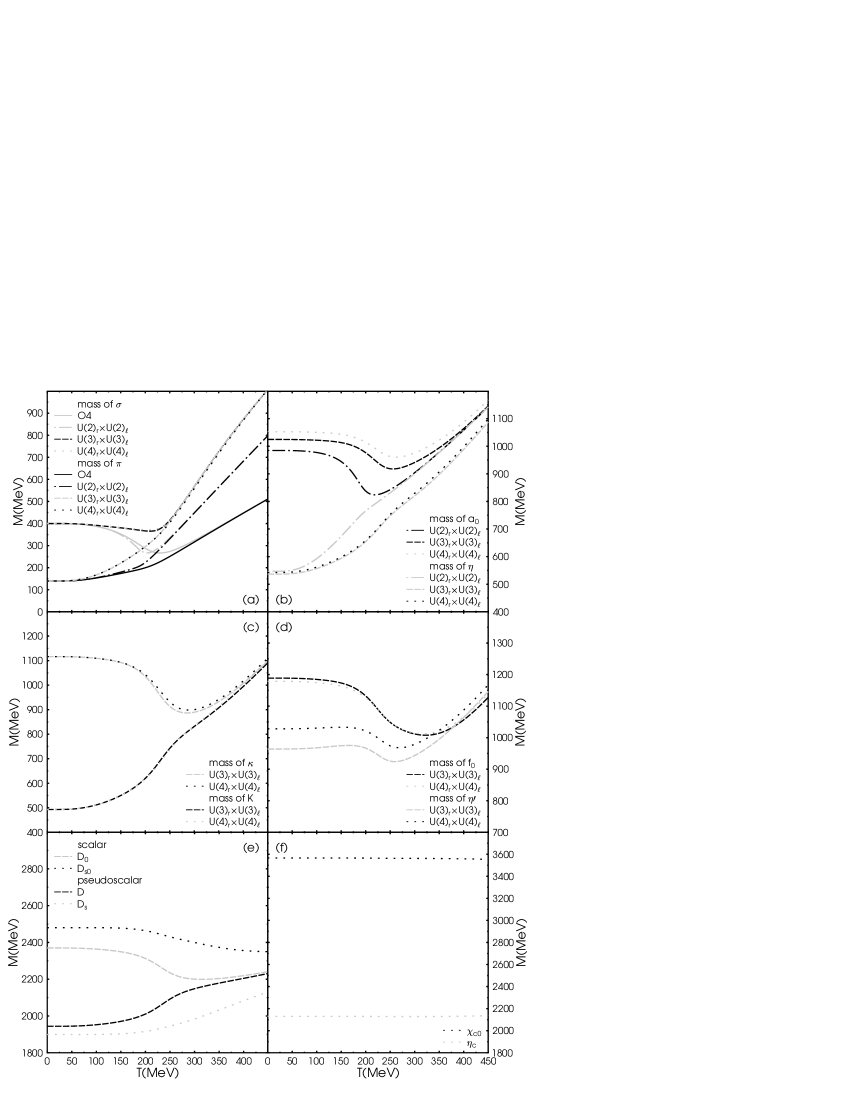
Figure 2: The meson masses as a function of temperature for the different models studied here, for the case with $U(1)_{A}$ anomaly and explicit chiral symmetry breaking.

IV.1 Explicit chiral symmetry breaking with $U(1)_{A}$ anomaly

In Fig. 2, we show the masses of the mesons as a function of temperature for explicit chiral symmetry breaking, including the $U(1)_{A}$ anomaly. This is the case where chiral symmetry breaking results in the smallest residual symmetry group, $SU(N_{f})_{V}\times U(N_{f})_{A}\rightarrow SU(2)_{V}$.

In Fig. 2(a) the masses of the $\sigma$ meson and the pions are shown for all models. The $\sigma$ meson and the pion become degenerate in mass in the chirally restored phase. Comparing the $\sigma$ meson and pion masses in the $O(4)$ model with those in the $U(2)_{r}\times U(2)_{\ell}$ model, the difference is almost negligible up to temperatures of 150 MeV. In the chirally restored phase, the masses behave linearly with temperature, but grow faster in the $U(2)_{r}\times U(2)_{\ell}$ model than in the $O(4)$ model. The reason is that there are twice as many fields in the former model than in the latter, which results in twice as many tadpole-like contributions in the equations for the in-medium masses. These come with a positive sign and thus increase the masses.

Comparing the results of the $U(3)_{r}\times U(3)_{\ell}$ model with those of the $U(2)_{r}\times U(2)_{\ell}$ model, one observes differences already at a temperature of about 100 MeV. Furthermore, the masses become even larger in the chirally restored phase. The reason for this behavior are the strange degrees of freedom in the $N_{f}=3$ case which lead to additional tadpole-like terms in the self-energies. As above, they lead to an increase of the in-medium masses.

Finally, one observes that virtually nothing changes in the temperature range of interest when including the charm degrees of freedom in the framework of the $U(4)_{r}\times U(4)_{\ell}$ model. The reason is that the charm quark is large compared to the temperature, $m_{c}\gg T$, and the contributions from charmed particles to the equations for the in-medium masses is suppressed. For two reasons, this is a non-trivial result. First, the equations for the in-medium masses are structurally different for the $U(4)_{r}\times U(4)_{\ell}$ model as compared to the $U(3)_{r}\times U(3)_{\ell}$ model, cf. Eqs. (25) and (36). Second, although the tadpole terms (39) are strongly suppressed for particles with masses much larger than the temperature, Eqs. (33) and (36) form a nonlinear system of coupled equations, i.e., small perturbations could lead to large quantitative changes in the solution.

In Fig. 2(b) the masses of the $a_{0}$ and the $\eta$ mesons are shown as functions of temperature. Qualitatively, the behavior of these masses is the same in all models. The $a_{0}$ meson mass is constant up to temperatures of 150 – 200 MeV. It then decreases, before increasing again above temperatures of 200 – 250 MeV. The $\eta$ meson mass is constant up to $T\simeq 50$ MeV, and then monotonously increases with temperature. At large temperatures, $a_{0}$ and $\eta$ become degenerate in mass, indicating restoration of chiral symmetry. In the $U(2)_{r}\times U(2)_{\ell}$ model, this happens somewhat earlier, at about 250 MeV, than in the other two cases.

In the $U(2)_{r}\times U(2)_{\ell}$ model, the $a_{0}$ and $\eta$ meson masses are used to determine the parameters of the model. Thus, at zero temperature, the masses coincide with their correct vacuum values. In the $U(3)_{r}\times U(3)_{\ell}$ model, the predicted $\eta$ mass deviates only by 2% from its vacuum value. The $a_{0}$ mass is also rather close to the correct value; the predicted mass is about 4% too large. In the $U(4)_{r}\times U(4)_{\ell}$, the $\eta$ mass is reproduced with excellent accuracy (the deviation is less than 1%), while the $a_{0}$ mass is within 7% of its vacuum value.

In Fig. 2(c) the $\kappa$ meson (now referred to as $K_{0}^{*}(1430)$ Hagiwara et al. (2002)) and kaon masses are shown as a function of temperature. The results for the $U(3)_{r}\times U(3)_{\ell}$ and $U(4)_{r}\times U(4)_{\ell}$ model are almost identical. The $\kappa$ meson and kaon become degenerate in mass at temperatures of the order of 400 MeV. In both models, the vacuum kaon mass is used as input, while the $\kappa$ mass is predicted. The deviation to the vacuum value in nature is about 21%.

Figure 2(d) shows the masses of the $f_{0}$ and the $\eta^{\prime}$ meson as a function of temperature. These mesons also become degenerate in mass at temperatures of the order of 400 MeV. In the $U(3)_{r}\times U(3)_{\ell}$ model, the predicted $\eta^{\prime}$ mass is rather close to its value in nature; the deviation is 0.6%. In the $U(4)_{r}\times U(4)_{\ell}$ model, the $\eta^{\prime}$ mass deviates from its correct vacuum value by about 7%. The $f_{0}$ mass is predicted in both models. If we identify this state with the $f_{0}(1370)$, these predicted masses deviate by 14% from their correct values.

The masses of the $D_{s0}$, $D_{0}$, $D_{s}$, and $D$ mesons are shown in Fig. 2(e). The masses of the pseudoscalar mesons are known but the scalar mesons and their masses have not yet been experimentally identified. It is somewhat peculiar that the charmed, strange $D_{s}$ meson is lighter than the charmed, non-strange $D$ meson. This is an artifact of the particular set of coupling constants chosen here. For a different choice, this unphysical ordering of the masses can be reversed. Then, however, the masses of the other mesons deviate by an unacceptably large extent from their physical values. Temperature has virtually no effect on the heavy charmed mesons: their mass changes at most by 10%, even in the chirally restored phase. Due to the non-linear nature of the coupled system of Eqs. (33) and (36), this is a non-trivial result, although not completely unexpected: we expect significant changes of the meson masses only when the temperature becomes of the order of the mass. For the charmed mesons with masses of the order of 2 GeV, this is never the case in the temperature range of interest.

Finally, in Fig. 2(f) we show the masses of the $\chi_{c0}$ and $\eta_{c}$ meson. Their large masses do not change at all for temperatures below 450 MeV. The vacuum values for both meson masses are predicted. While the mass for the $\chi_{c0}$ is within 5% of its correct value, the deviation for the $\eta_{c}$ is somewhat larger ($\simeq 30\%$).

To summarize, the masses of the scalar mesons remain approximately constant up to temperatures around 150 MeV, and then slightly decrease before they become degenerate with the masses of the pseudoscalar mesons. On the other hand, with the exception of the $\eta^{\prime}$ mass, the pseudoscalar masses in general increase monotonously with temperature.

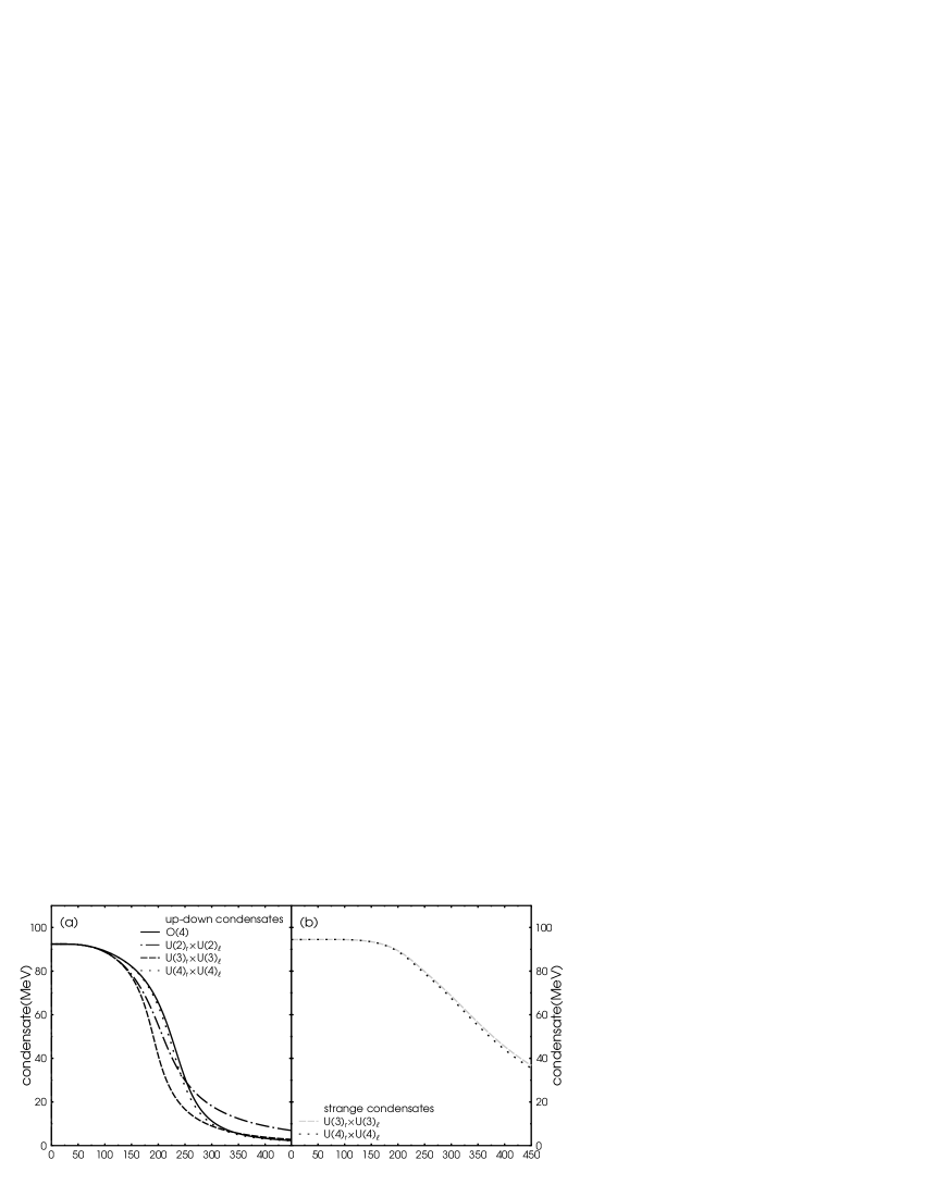
Figure 3: (a) The up-down quark condensate and (b) the strange quark condensate as functions of temperature for the different models in the case with $U(1)_{A}$ anomaly and explicitly broken chiral symmetry.

In Fig. 3(a) the up-down quark condensate and (b) the strange quark condensate are shown as functions of temperature. In the $O(4)$ model and in the $U(2)_{r}\times U(2)_{\ell}$ model the up-down quark condensate $\varphi_{\rm up-down}$ can be directly identified with the vacuum expectation value of the $\sigma$ field, $\varphi_{\rm up-down}\equiv\sigma_{0}$. On the other hand, in the $U(3)_{r}\times U(3)_{\ell}$ model Lenaghan et al. (2000),

$$\varphi_{\rm up-down} = \sqrt{\frac{2}{3}}\,\sigma_{0}+\frac{1}{\sqrt{3}}\,\sigma_{8}\,\,,$$ (50a)

$$\varphi_{\rm strange} = \frac{1}{\sqrt{3}}\,\sigma_{0}-\sqrt{\frac{2}{3}}\,\sigma_{8}\,\,,$$ (50b)

and in the $U(4)_{r}\times U(4)_{\ell}$ model the condensates are given by

$$\varphi_{\rm up-down} = \frac{1}{\sqrt{2}}\,\sigma_{0}+\frac{1}{\sqrt{3}}\,\sigma_{8}+\frac{1}{\sqrt{6}}\,\sigma_{15}\,\,,$$ (51a)

$$\varphi_{\rm strange} = \frac{1}{2}\,\sigma_{0}-\sqrt{\frac{2}{3}}\,\sigma_{8}+\frac{1}{2\sqrt{3}}\,\sigma_{15}\,\,,$$ (51b)

$$\varphi_{\rm charm} = \frac{1}{2}\,\sigma_{0}-\frac{\sqrt{3}}{2}\,\sigma_{15}\,\,.$$ (51c)

In these formulas $\varphi_{\rm strange}$ and $\varphi_{\rm charm}$ are the strange and charm quark condensate, respectively.

All models predict a qualitatively similar behavior for the temperature dependence of the up-down quark condensates. The strange quark condensate decreases more slowly with temperature than the up-down quark condensate. This is what one intuitively expects, as it appears more difficult to “melt” a condensate of heavier quark species than of light quark species.

Figure 4: The charm quark condensate as a function of temperature.

Figure 4 shows the charm quark condensate. Note that this condensate is much larger than the other two condensates. A peculiar feature is that it first increases at a temperature of about 200 MeV, assumes a maximum at about 400 MeV, and then decreases. The maximum value is approximately 10% larger than the vacuum value. We are not aware of a simple explanation for this behavior.

IV.2 Explicit chiral symmetry breaking without $U(1)_{A}$ anomaly

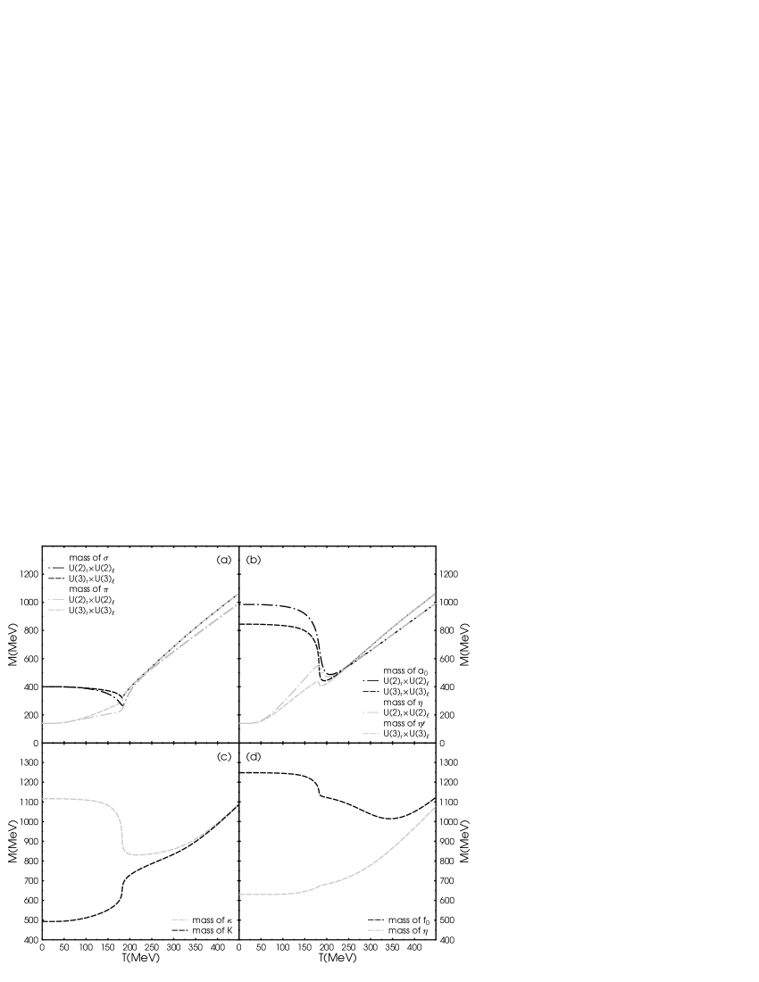
Figure 5: The meson masses as a function of temperature for the different models in the case without $U(1)_{A}$ anomaly and explicit chiral symmetry breaking.

In Fig. 5, we show the masses for the scalar and pseudoscalar mesons for the case of explicit chiral symmetry breaking in the absence of the $U(1)_{A}$ anomaly. We discuss the results in comparison to the previous case. As in the previous case, the scalar meson masses stay constant up to temperatures close to the transition region, then decrease and finally start to increase again when they become degenerate with the pseudoscalar masses. In general, the pseudoscalar masses increase monotonously with temperature. The difference between the results obtained in the $U(2)_{r}\times U(2)_{\ell}$ and $U(3)_{r}\times U(3)_{\ell}$ model is rather small. An exception is the $a_{0}$ mass which is an input parameter in the former model, but is predicted in the latter.

A marked difference to the case with $U(1)_{A}$ anomaly is that the chiral symmetry restoration transition is much more rapid, and it occurs at a slightly smaller temperature, $T\simeq 180$ MeV. Moreover, above the transition the scalar and pseudoscalar masses become degenerate much more rapidly. The reason is the absence of explicit $U(1)_{A}$ symmetry breaking. At small temperatures and above the transition, the masses of the pion and the $\eta$ meson are the same, because of the absence of the $U(1)_{\rm A}$ anomaly. In the temperature range from about $50$ MeV to $225$ MeV, however, they are different. We believe this to be an artifact originating from the violation of Goldstone’s theorem in the Hartree approximation, which becomes even more obvious when considering the chiral limit.

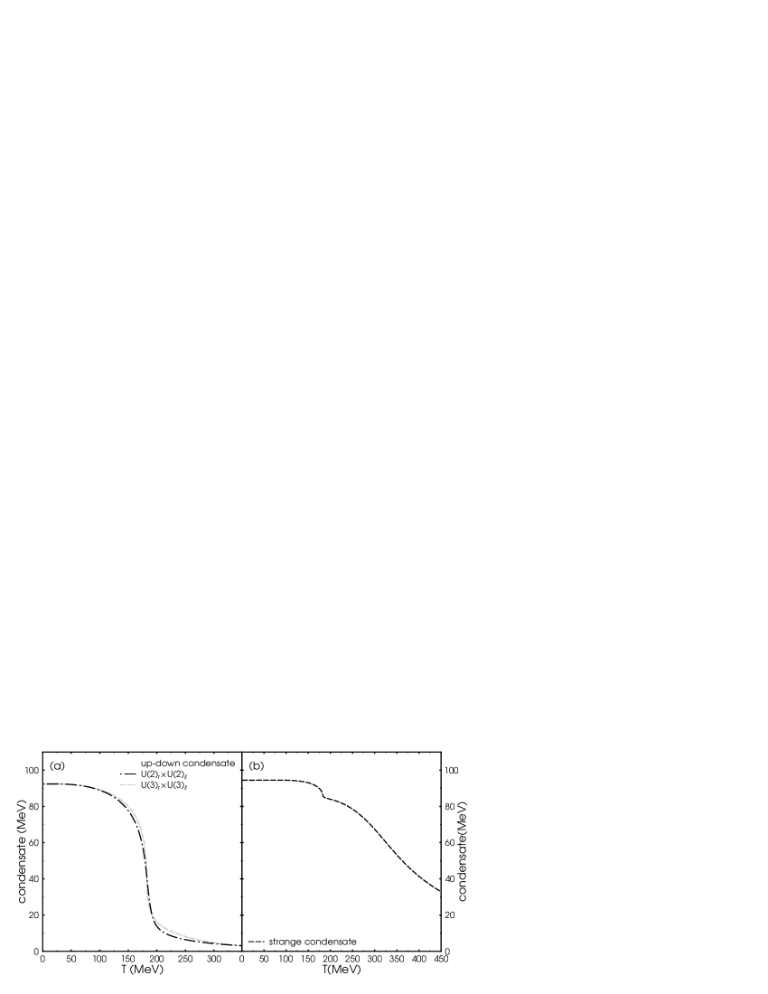
Figure 6: (a) The up-down quark condensate and (b) the strange quark condensate as a function of temperature for the different models in the case without $U(1)_{A}$ anomaly and explicitly broken chiral symmetry.

The melting of the condensates is shown in Fig. 6. The smaller transition temperature of about $180$ MeV is also apparent in the temperature dependence of the up-down quark condensate. Again, the strange quark condensate melts less rapidly than the up-down quark condensate.

IV.3 Chiral limit with $U(1)_{A}$ anomaly

Figure 7: The chiral limit with $U(1)_{A}$ anomaly. The temperature dependence of the meson masses are shown in panels $(~{},1)$ and that of the up-down and strange quark condensates in panels $(~{},3)$. The results for the $O(4)$ model are shown in panels $(a,~{})$, for the $U(2)_{r}\times U(2)_{\ell}$ model in panels $(b,~{})$, and for the $U(3)_{r}\times U(3)_{\ell}$ model in panels $(c,~{})$. The effective potential (in arbitrary units) as a function of the condensate $\sigma_{0}$ is shown in panels $(~{},2)$.

The masses as a function of temperature for the $O(4)$ model are shown in Fig. 7(a,1), for the $U(2)_{r}\times U(2)_{\ell}$ model in Fig. 7(b,1), and for the $U(3)_{r}\times U(3)_{\ell}$ model in Fig. 7(c,1). In the $O(4)$ and $U(2)_{r}\times U(2)_{\ell}$ models, there are three Goldstone bosons, the pions, while in the $U(3)_{r}\times U(3)_{\ell}$ model there are eight Goldstone bosons, the pions, the kaons, and the $\eta$ meson. The $\eta^{\prime}$ meson is not a Goldstone boson due to the explicit breaking of the $U(1)_{A}$ symmetry by the anomaly. The scalar octet, comprising the three $a_{0}$ mesons, the four $\kappa$ mesons, and the $f_{0}$ meson, is degenerate in mass, while the mass of the singlet $\sigma$ differs from the mass of the octet. As the temperature increases, the scalar masses decrease while the pseudoscalar masses increase. The mass of the Goldstone bosons increases, because the Hartree approximation does not respect Goldstone’s theorem at nonzero temperature Lenaghan and Rischke (2000); Lenaghan et al. (2000).

Due to the restoration of chiral symmetry above the transition temperature $T_{c}$, the masses of the chiral partners become degenerate for temperatures $T>T_{c}$. For the $O(4)$ model, the chiral partners are the $\sigma$ and the pion, for the $U(2)_{r}\times U(2)_{\ell}$ model they are the $\sigma$ and the pion, as well as the $a_{0}$ and the $\eta$. Due to the explicit breaking of the $U(1)_{A}$ symmetry, the $\sigma/$pion and $a_{0}/\eta$ do not become degenerate. The reason for this behavior is the term $\sim{\cal G}_{ab}$ in Eqs. (25). As discussed in Sec. III.2, at zero temperature this term leads to a difference in the masses (squared) of $\eta$ meson and pion, and of the $a_{0}$ and $\sigma$ meson, respectively, which is proportional to $2c$. In the case with $U(1)_{A}$ anomaly, $2c\neq 0$ even for temperatures above $T_{c}$. Consequently, these mass differences persist also in the chirally restored phase.

For $N_{f}=3$, the situation is different. The term $\sim{\cal G}_{ab}$ for $N_{f}=2$ is replaced by a term $\sim{\cal G}_{abc}\sigma_{c}$. In the chirally symmetric phase, $\sigma_{c}=0$, and consequently this term vanishes. Therefore, all meson masses become degenerate, even in the case with $U(1)_{A}$ anomaly.

All models exhibit a first order phase transition between the low-temperature phase where chiral symmetry is broken and the high-temperature phase where chiral symmetry is restored. For the $O(4)$ model and the $U(2)_{r}\times U(2)_{\ell}$ model with explicit breaking of the $U(1)_{A}$ symmetry, the transition should be second order, cf. Sec. I. It is a known shortcoming of the Hartree approximation to predict a first order transition also in these cases. For the $U(2)_{r}\times U(2)_{\ell}$ model without explicit breaking of the $U(1)_{A}$ symmetry, and for all $U(N_{f})_{r}\times U(N_{f})_{\ell}$ models with $N_{f}>2$ the transition is of first order, which is correctly reproduced by the Hartree approximation.

We have determined the numerical value of $T_{c}$ by computing the effective potentials. The latter are shown for the three different models in the second column of Fig. 7 as a function of the condensate $\sigma_{0}$. (In the chiral limit, $\sigma_{0}$ is the only non-trivial condensate.) For the extraction of the transition temperature, the absolute normalization of the effective potential is irrelevant. All that matters is to identify the temperature where the minimum at the origin and the one at a nonzero value of $\sigma_{0}$ become degenerate. For this purpose we have plotted the effective potential for two temperatures, one slightly below and one slightly above $T_{c}$. From this we deduce that, for the $O(4)$ model, Fig. 7(a,2), $T_{c}$ is between 159 and 160 MeV. For the $U(2)_{r}\times U(2)_{\ell}$ model, Fig. 7(b,2), we obtain a critical temperature between 154 and 155 MeV. This temperature is rather close to the one in the $O(4)$ model. Finally, for the $U(3)_{r}\times U(3)_{\ell}$ model, the critical temperature is between 165 and 166 MeV, which is slightly larger than in the previous cases.

These values are surprisingly close to those obtained from lattice QCD calculations Karsch (2002). In the chiral limit, these calculations predict $T_{c}\simeq 175$ MeV for $N_{f}=2$ and $T_{c}\simeq 155$ MeV for $N_{f}=3$. The critical temperature obtained from the chiral models in the Hartree approximation deviates from these values only by about 20 MeV (or 12%) for $N_{f}=2$ and only 10 MeV (or 6%) for $N_{f}=3$. However, for the chiral models the transition temperature is larger in the three-flavor case than in the two-flavor case, while one finds the opposite behavior in the lattice QCD calculations.

For the sake of completeness we also show the condensates in the third column of Fig. 7. Note that, in contrast to the cases where chiral symmetry is explicitly broken, the strange condensate is smaller than the up-down condensate. The reason is that, in the chiral limit, $\sigma_{8}=0$, such that $\varphi_{\rm up-down}=\sqrt{2}\,\varphi_{\rm strange}$, cf. Eq. (50).

IV.4 Chiral limit without $U(1)_{A}$ anomaly

Figure 8: The chiral limit without $U(1)_{A}$ anomaly. The temperature dependence of the meson masses are shown in panels $(~{},1)$ and that of the up-down and strange quark condensates in panels $(~{},3)$. The results for the $U(2)_{r}\times U(2)_{\ell}$ model in panels $(a,~{})$, and for the $U(3)_{r}\times U(3)_{\ell}$ model in panels $(b,~{})$. The effective potential (in arbitrary units) as a function of the condensate $\sigma_{0}$ is shown in panels $(~{},2)$.

The masses as a function of temperature are shown in Fig. 8(a,1) for the $U(2)_{r}\times U(2)_{\ell}$ model, and in Fig. 8(b,1) for the $U(3)_{r}\times U(3)_{\ell}$ model. In the first case, there are four Goldstone bosons, the pions and the $\eta$ meson, while in the latter case there are nine Goldstone bosons, the pions, the kaons, and the $\eta$ and $\eta^{\prime}$ mesons. As the temperature increases, the scalar masses decrease while the pseudoscalar masses increase, until they become degenerate in a first order phase transition. The mass of the Goldstone bosons increases with temperature, because the Hartree approximation does not respect Goldstone’s theorem at nonzero temperature Lenaghan and Rischke (2000); Lenaghan et al. (2000). Moreover, the masses of the Goldstone bosons are not equal: for the $U(2)_{r}\times U(2)_{\ell}$ model, the $\eta$ meson becomes heavier than the pion, while for the $U(3)_{r}\times U(3)_{\ell}$ model the $\eta^{\prime}$ meson becomes heavier than the other Goldstone bosons (pions, kaons, $\eta$ meson). Note that the role of the $\eta$ meson in the two-flavor case is assumed by the $\eta^{\prime}$ meson in the three-flavor case. The reason is that the physical meson corresponding to the singlet representation in the $U(2)_{r}\times U(2)_{\ell}$ model is the $\eta$ meson, while it is the $\eta^{\prime}$ in the $U(3)_{r}\times U(3)_{\ell}$ model.

The numerical values for the critical temperature $T_{c}$ have been determined by computing the effective potentials. The latter are shown in the second column of Fig. 8 as a a function of the condensate $\sigma_{0}$, for temperatures slightly below and above $T_{c}$. In the $U(2)_{r}\times U(2)_{\ell}$ model, Fig. 8(a,2) we obtain a critical temperature of $\simeq 150$ MeV. For the $U(3)_{r}\times U(3)_{\ell}$ model the temperature is slightly smaller, between 147 and 148 MeV. The ordering of critical temperatures for the two- and three-flavor cases is now reversed as compared to the case with $U(1)_{A}$ anomaly, and consequently in agreement with the ordering found in lattice QCD calculations. One might be tempted to view this as an indication for a rapidly decreasing $U(1)_{A}$ anomaly near the critical temperature, in agreement with the results of Ref. Alles et al. (1997); Schaffner-Bielich (2000). Finally, the condensates are shown in the third column of Fig. 8. The results are qualitatively similar to the case with $U(1)_{A}$ anomaly.

V Conclusions

In this work, we have used several different chiral models, the $O(4)$, the $U(2)_{r}\times U(2)_{\ell}$, the $U(3)_{r}\times U(3)_{\ell}$, and the $U(4)_{r}\times U(4)_{\ell}$ linear sigma model, to compute the temperature dependence of meson masses and quark condensates across the chiral phase transition. The meson masses and condensates were self-consistently calculated in the Hartree approximation, which we derived via the CJT formalism. Moreover, we have studied several distinct patterns of symmetry breaking within the different models. For a list of cases studied here see Table 1.

We first considered the physically relevant case of explicit symmetry breaking in the presence of the $U(1)_{A}$ anomaly and compared the results of the different chiral models in order to clarify how they change with the number of quark flavors $N_{f}$. Comparing the $O(4)$ model with the $U(2)_{r}\times U(2)_{\ell}$ model, one first notices that the degrees of freedom have doubled: in addition to the $\sigma$ meson and the pions which are already present in the $O(4)$ model, one now has in addition the $\eta$ meson and the $a_{0}$ mesons. This has the consequence that the meson masses grow more rapidly with temperature in the phase where chiral symmetry is restored. The reason for this are the tadpole contributions from the additional degrees of freedom to the meson self-energies, which lead to an increase in the meson masses. This result also applies when adding the strange degree of freedom in the framework of the $U(3)_{r}\times U(3)_{\ell}$ model. In fact, this picture holds in general, as long as the masses of the additional degrees of freedom are of the same order of magnitude as the chiral phase transition temperature. On the other hand, adding the heavy charm quark degree of freedom in the framework of the $U(4)_{r}\times U(4)_{\ell}$ model does not significantly influence the results for the masses of the non-charmed mesons and the non-charmed condensates. The reason is that the additional tadpole contributions from the heavy charmed mesons are exponentially suppressed with the meson mass, $\sim\exp(-M/T)$. Vice versa, also the masses of the charmed mesons do not change appreciably from their vacuum values over the range of temperatures of interest for chiral symmetry restoration, simply because the tadpole contributions from the non-charmed meson are small compared to the large vacuum mass of the charmed mesons. This result is intuitively clear from the physical point of view, but is still non-trivial: first, the equations for the in-medium masses are structurally different for the $U(4)_{r}\times U(4)_{\ell}$ model as compared to the $U(3)_{r}\times U(3)_{\ell}$ model. Second, the set of coupled equations for the masses and condensates is a nonlinear system of equations, which means that small perturbations could lead to large quantitative changes in the solution.

We then studied the case of explicit chiral symmetry breaking without $U(1)_{A}$ anomaly. The main difference to the previous case was that the region of the chiral transition is narrower and located at a somewhat smaller temperature.

Finally, we considered the meson masses and quark condensates in the chiral limit. The Hartree approximation correctly predicts the chiral transition to be of first order in the $U(2)_{r}\times U(2)_{\ell}$ model without $U(1)_{A}$ anomaly and in the $U(3)_{r}\times U(3)_{\ell}$ model. For the $O(4)$ model and the $U(2)_{r}\times U(2)_{\ell}$ model with $U(1)_{A}$ anomaly the Hartree approximation incorrectly produces a first order instead of a second order phase transition. The transition temperatures are surprisingly close to the ones obtained in lattice QCD calculations. However, in the case with $U(1)_{A}$ anomaly the transition temperature increases with the number of flavors, while in lattice QCD it decreases. This picture changes in the case with $U(1)_{A}$ anomaly, where the transition temperature shows the same behavior with the number of quark flavors as in lattice QCD. This may indicate that the $U(1)_{A}$ symmetry is, at least partially, restored at and above the chiral phase transition temperature.

Appendix A Scalar and pseudoscalar meson fields

For $N_{f}=2$, the identification of the physical scalar and pseudoscalar meson fields with the matrix fields defined in Eq. (19a) is

$$T_{a}\sigma_{a} = \frac{1}{\sqrt{2}}\left(\begin{array}[]{ccc}\frac{1}{\sqrt{2}}\sigma_{0}+\frac{1}{\sqrt{2}}a_{0}^{0}&a_{0}^{+}\\ a_{0}^{-}&\frac{1}{\sqrt{2}}\sigma_{0}-\frac{1}{\sqrt{2}}a_{0}^{0}\\ \end{array}\right)\,\,,$$ (52c)

$$T_{a}\pi_{a} = \frac{1}{\sqrt{2}}\left(\begin{array}[]{ccc}\frac{1}{\sqrt{2}}\pi_{0}+\frac{1}{\sqrt{2}}\pi^{0}&\pi^{+}\\ \pi^{-}&\frac{1}{\sqrt{2}}\pi_{0}-\frac{1}{\sqrt{2}}\pi^{0}\\ \end{array}\right)\,\,.$$ (52f)

Here, $\pi^{\pm}\equiv(\pi_{1}\mp i\pi_{2})/\sqrt{2}$ and $\pi^{0}\equiv\pi_{3}$ are the charged and neutral pions, respectively. Note the change of sign in the definition of the charged pion fields $\pi^{\pm}$ in terms of $\pi_{1,2}$ in comparison to Ref. Lenaghan et al. (2000). The definition given here is the correct one, as one can readily confirm by writing the meson fields in terms of their quark content,

$$\pi_{a}\sim\bar{q}\,T_{a}\,\gamma_{5}\,q\,\,.$$ (53)

This applies also to the other charged meson fields defined in the following. The field $\eta\equiv\pi_{0}$ can be identified with the $\eta$ meson. The parity partner of the pion is the $a_{0}$(980) meson, i.e., $a_{0}^{\pm}\equiv(\sigma_{1}\mp i\sigma_{2})/\sqrt{2}$ and $a_{0}^{0}\equiv\sigma_{3}$. The field $\sigma_{0}$ corresponds to the $\sigma$ meson [now also referred to as $f_{0}(400-1200)$].

For $N_{f}=3$ we obtain the following matrix:

$$T_{a}\sigma_{a} = \frac{1}{\sqrt{2}}\left(\begin{array}[]{ccc}\frac{1}{\sqrt{2}}a_{0}^{0}+\frac{1}{\sqrt{6}}\sigma_{8}+\frac{1}{\sqrt{3}}\sigma_{0}&{a_{0}^{+}}&\kappa^{+}\\ a_{0}^{-}&-\frac{1}{\sqrt{2}}a_{0}^{0}+\frac{1}{\sqrt{6}}\sigma_{8}+\frac{1}{\sqrt{3}}\sigma_{0}&\kappa^{0}\\ \kappa^{-}&\bar{\kappa^{0}}&-\frac{2}{\sqrt{3}}\sigma_{8}+\frac{1}{\sqrt{3}}\sigma_{0}\\ \end{array}\right)\,\,,$$ (54d)

$$T_{a}\pi_{a} = \frac{1}{\sqrt{2}}\left(\begin{array}[]{ccc}\frac{1}{\sqrt{2}}\pi^{0}+\frac{1}{\sqrt{6}}\pi_{8}+\frac{1}{\sqrt{3}}\pi_{0}&\pi^{+}&K^{+}\\ \pi^{-}&-\frac{1}{\sqrt{2}}\pi^{0}+\frac{1}{\sqrt{6}}\pi_{8}+\frac{1}{\sqrt{3}}\pi_{0}&K^{0}\\ K^{-}&\bar{K^{0}}&-\frac{2}{\sqrt{3}}\pi_{8}+\frac{1}{\sqrt{3}}\pi_{0}\\ \end{array}\right)\,\,.$$ (54h)

The fields $K^{\pm}\equiv(\pi_{4}\mp i\,\pi_{5})/\sqrt{2}$, $K^{0}\equiv(\pi_{6}-i\,\pi_{7})/\sqrt{2}$, and $\bar{K}^{0}\equiv(\pi_{6}+i\,\pi_{7})/\sqrt{2}$ are the kaons. In general, because the strange quark is much heavier than the up or down quarks, the $\pi_{0}$ and the $\pi_{8}$ are admixtures of the $\eta$ and the $\eta^{\prime}$ meson. We identify the parity partner of the kaon with the $\kappa$ meson [now referred to as $K_{0}^{*}(1430)$ in Hagiwara et al. (2002)]. Finally, in general the $\sigma_{0}$ and the $\sigma_{8}$ are admixtures of the $\sigma$ and $f_{0}(980)$ mesons.

For $N_{f}=4$ the following identification of physical fields with matrix elements holds:

$$T_{a}\sigma_{a} = \frac{1}{\sqrt{2}}\left(\begin{array}[]{cccc}{A_{S}}&{a_{0}^{+}}&{\kappa^{+}}&{\bar{D}^{0}_{0}}\\ {a_{0}^{-}}&{B_{S}}&{\kappa^{0}}&{D^{-}_{0}}\\ {\kappa^{-}}&{\bar{\kappa}^{0}}&{C_{S}}&{D^{-}_{s,0}}\\ {D^{0}_{0}}&{D^{+}_{0}}&{D^{+}_{s,0}}&{D_{S}}\\ \end{array}\right)\,\,,$$ (59)

where

$$A_{S} = \frac{1}{2}\sigma_{0}+\frac{1}{\sqrt{2}}a_{0}^{0}+\frac{1}{\sqrt{6}}\sigma_{8}+\frac{1}{\sqrt{12}}\sigma_{15}\,\,,$$

$$B_{S} = \frac{1}{2}\sigma_{0}-\frac{1}{\sqrt{2}}a_{0}^{0}+\frac{1}{\sqrt{6}}\sigma_{8}+\frac{1}{\sqrt{12}}\sigma_{15}\,\,,$$

$$C_{S} = \frac{1}{2}\sigma_{0}-\frac{2}{\sqrt{6}}\sigma_{8}+\frac{1}{\sqrt{12}}\sigma_{15}\,\,,$$

$$D_{S} = \frac{1}{2}\sigma_{0}-\frac{3}{\sqrt{12}}\sigma_{15}\,\,,$$

and

$$T_{a}\pi_{a} = \frac{1}{\sqrt{2}}\left(\begin{array}[]{cccc}{A_{P}}&{\pi^{+}}&{K^{+}}&{\bar{D}^{0}}\\ {\pi^{-}}&{B_{P}}&{K^{0}}&{D^{-}}\\ {K^{-}}&{\bar{K}^{0}}&{C_{P}}&{D^{-}_{s}}\\ {D^{0}}&{D^{+}}&{D^{+}_{s}}&{D_{P}}\\ \end{array}\right)\,\,,$$ (64)

with

$$A_{P} = \frac{1}{2}\pi_{0}+\frac{1}{\sqrt{2}}\pi^{0}+\frac{1}{\sqrt{6}}\pi_{8}+\frac{1}{\sqrt{12}}\pi_{15}\,\,,$$

$$B_{P} = \frac{1}{2}\pi_{0}-\frac{1}{\sqrt{2}}\pi^{0}+\frac{1}{\sqrt{6}}\pi_{8}+\frac{1}{\sqrt{12}}\pi_{15}\,\,,$$

$$C_{P} = \frac{1}{2}\pi_{0}-\frac{2}{\sqrt{6}}\pi_{8}+\frac{1}{\sqrt{12}}\pi_{15}\,\,,$$

$$D_{P} = \frac{1}{2}\pi_{0}-\frac{3}{\sqrt{12}}\pi_{15}\,\,.$$

Here, $D^{0}=(\pi_{9}+i\pi_{10})/\sqrt{2}$, $\bar{D}^{0}=(\pi_{9}-i\pi_{10})/\sqrt{2}$, $D^{\pm}=(\pi_{11}\pm i\pi_{12})/\sqrt{2}$, and $D^{\pm}_{s}=(\pi_{13}\pm i\pi_{14})/\sqrt{2}$ are the charged and neutral pseudoscalar mesons with charm quantum numbers. The $\pi_{0}$, $\pi_{8}$, and $\pi_{15}$ fields are admixtures of the $\eta$, $\eta^{\prime}$, and $\eta_{c}$ mesons. The charged and neutral scalar mesons with charm quantum numbers are $D_{0}^{0}=(\sigma_{9}+i\sigma_{10})/\sqrt{2}$, $\bar{D}_{0}^{0}=(\sigma_{9}-i\sigma_{10})/\sqrt{2}$, $D_{0}^{\pm}=(\sigma_{11}\pm i\sigma_{12})/\sqrt{2}$, and $D_{s,0}^{\pm}=(\sigma_{13}\pm i\sigma_{14})/\sqrt{2}$. These scalar mesons have not been identified experimentally, yet. The $\sigma_{0}$, $\sigma_{8}$, and $\sigma_{15}$ fields are admixtures of the $\sigma$, $f_{0}$, and $\chi_{c0}$ mesons.

References

- ’t Hooft (1976a) G. ’t Hooft, Phys. Rev. D14, 3432 (1976a).
- ’t Hooft (1976b) G. ’t Hooft, Phys. Rev. Lett. 37, 8 (1976b).
- Pisarski and Wilczek (1984) R. D. Pisarski and F. Wilczek, Phys. Rev. D29, 338 (1984).
- Karsch (2002) F. Karsch, Lect. Notes Phys. 583, 209 (2002), eprint [http://arXiv.org/abs]hep-lat/0106019.
- Brown et al. (1990) F. R. Brown et al., Phys. Rev. Lett. 65, 2491 (1990).
- Iwasaki et al. (1996) Y. Iwasaki, K. Kanaya, S. Kaya, S. Sakai, and T. Yoshie, Z. Phys. C71, 343 (1996), eprint [http://arXiv.org/abs]hep-lat/9505017.
- Lenaghan (2001) J. T. Lenaghan, Phys. Rev. D63, 037901 (2001), eprint [http://arXiv.org/abs]hep-ph/0005330.
- Dolan and Jackiw (1974) L. Dolan and R. Jackiw, Phys. Rev. D9, 3320 (1974).
- Lenaghan et al. (2000) J. T. Lenaghan, D. H. Rischke, and J. Schaffner-Bielich, Phys. Rev. D62, 085008 (2000), eprint [http://arXiv.org/abs]nucl-th/0004006.
- Lenaghan and Rischke (2000) J. T. Lenaghan and D. H. Rischke, J. Phys. G26, 431 (2000), eprint [http://arXiv.org/abs]nucl-th/9901049.
- Gell-Mann and Levy (1960) M. Gell-Mann and M. Levy, Nuovo Cim. 16, 705 (1960).
- Petropoulos (1999) N. Petropoulos, J. Phys. G25, 2225 (1999), eprint [http://arXiv.org/abs]hep-ph/9807331.
- Cornwall et al. (1974) J. M. Cornwall, R. Jackiw, and E. Tomboulis, Phys. Rev. D10, 2428 (1974).
- van Hees and Knoll (2000) H. van Hees and J. Knoll, Nucl. Phys. A683, 369 (2000), eprint [http://arXiv.org/abs]hep-ph/0007070.
- van Hees and Knoll (2002) H. van Hees and J. Knoll, Phys. Rev. D65, 025010 (2002), eprint [http://arXiv.org/abs]hep-ph/0107200.
- Van Hees and Knoll (2002) H. Van Hees and J. Knoll, Phys. Rev. D65, 105005 (2002), eprint [http://arXiv.org/abs]hep-ph/0111193.
- van Hees and Knoll (2002) H. van Hees and J. Knoll, Phys. Rev. D66, 025028 (2002), eprint [http://arXiv.org/abs]hep-ph/0203008.
- Jackiw (1974) R. Jackiw, Phys. Rev. D9, 1686 (1974).
- Levy (1967) M. Levy, Nuovo Cim. 52, 23 (1967).
- Hu (1974) B. Hu, Phys. Rev. D9, 1825 (1974).
- Schechter and Singer (1975) J. Schechter and M. Singer, Phys. Rev. D12, 2781 (1975).
- Geddes (1980) H. B. Geddes, Phys. Rev. D21, 278 (1980).
- Vafa and Witten (1984) C. Vafa and E. Witten, Nucl. Phys. B234, 173 (1984).
- Hagiwara et al. (2002) K. Hagiwara et al. (Particle Data Group), Phys. Rev. D66, 010001 (2002).
- Alles et al. (1997) B. Alles, M. D’Elia, and A. Di Giacomo, Nucl. Phys. B494, 281 (1997), eprint hep-lat/9605013.
- Schaffner-Bielich (2000) J. Schaffner-Bielich, Phys. Rev. Lett. 84, 3261 (2000), eprint hep-ph/9906361.