CERN-TH/2003-014

On energy densities reached in
heavy-ion collisions at the CERN SPS

Ján Pišút^a,b, Neva Pišútová^b, and Boris Tomášik^a

^aCERN, Theory Division, CH-1211 Geneva 23, Switzerland

^bDepartment of Physics, Comenius University, SK-84248 Bratislava, Slovakia

March 13, 2003

1 Introduction

There exist plenty of models and Monte Carlo generators of proton–proton (pp), proton–nucleus (pA) and nucleus–nucleus (AB) interactions. These include models based on strings and their fragmentation, e.g. [1, 2, 3, 4], on partonic cascades [5, 6], on hadronic cascades [7, 8], on combined parton and hadron degrees of freedom [9], and on other pictures of the initial state of the collision. After fixing a few parameters, these models are able to find a reasonable agreement with data.

Another class of models for pA interactions is based on successive collisions of the incident proton with those nucleons in A which are present within a tube in A given by the trajectory of the proton in the nucleus and by the non-diffractive cross-section for proton–nucleon interaction, e.g. [10, 11, 12, 13, 14, 15, 16, 17, 18, 19, 20]. The model can be naturally extended to AB interactions. There it is based on the Glauber picture of colliding tubes of nucleons, see e.g. [11, 12, 13, 14, 15, 16, 17]. Models of this type proceed at every step in accordance with the data available from pp and pA interactions. A crucial input comes from data on the formation time of hadrons and on the Drell–Yan process [21]. Such a method keeps the parameters under control and gains some information about the space-time evolution of the process.

One of the most important quantities of interest in heavy-ion collisions is the highest energy density reached. This quantity is relevant to the possible approach to the quark–gluon plasma. In this paper we estimate the energy density reached at the CERN SPS by using a simple version of the Glauber-type model with tube-on-tube interactions.

We shall compare our estimates with recent lattice gauge theory results [22, 23]. The lattice results have brought a new and most interesting information on the type and parameters of the phase transition between the quark-gluon plasma (QGP) and the hadron gas (HG). The phase transition is most likely of a cross-over type, with critical temperature $T_{c}\approx 173\,\mbox{MeV}$ and the rather low critical energy density of $\varepsilon_{c}=\varepsilon(T_{c})\approx 0.7\,\mbox{GeV/fm}^{3}$.

The paper is organized as follows. In Section 2 we describe a simple version of the Glauber-type model of AB interactions, which we use in our calculations of rapidity distribution of the energy $\Delta E/\Delta y$. We also present our estimate of the volume occupied by the central rapidity region of $\Delta y\approx 1$ right after the tube-on-tube interaction is finished. The energy density is then estimated as the ratio of $\Delta E/\Delta y$ and $\Delta V/\Delta y$. More details of the model are explained in Section 3. In particular we discuss the formation time of hadrons and its relationship to the space-time picture of subsequent energy losses of incident nucleons in a tube-on-tube interaction. In Section 4 we present our results. Comments and concluding remarks are deferred to the last section.

2 The model

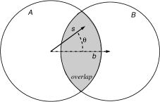
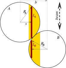
Figure 1: Left: geometry of non-central nuclear collisions. Right: layout of tube-on-tube interaction (plotted without Lorentz contraction).

For the sake of simplicity we shall take the nuclei as hard spheres with radii $R_{A}=1.2A^{1/3}$ fm and homogeneous number density $\rho=0.138\,\mbox{fm}^{-3}$. In the transverse plane, the impact parameter is denoted as $\vec{b}$ and a point in the transverse plane of the nucleus A is specified by the transverse coordinate $\vec{s}$. The angle between $\vec{b}$ and $\vec{s}$ is denoted as $\theta$. The situation is sketched in Fig. 1. In a Glauber model, the first part of the nuclear collision is described as a sum of tube-on-tube interactions (Fig. 1). In our model we will be interested in the energy density contained in such tubes just after the interaction.

The cross-section of both tubes is equal to the non-diffractive nucleon–nucleon cross-section $\sigma=30\,\mbox{mb}=3\,\mbox{fm}^{2}$. The lengths of the tubes $2L_{A}$ and $2L_{B}$ are given by

$$2L_{A}(s) = 2\sqrt{R_{A}^{2}-s^{2}}\,,$$ (1)

$$2L_{B}(b,s,\theta) = 2\sqrt{R_{B}^{2}-b^{2}-s^{2}+2bs\cos\theta}\,.$$ (2)

The average numbers of nucleons in both tubes are

$$\langle n_{A}(s)\rangle=2L_{A}(s)\rho\sigma,\quad\langle n_{B}(b,s,\theta)\rangle=2L_{B}(b,s,\theta)\rho\sigma\,.$$ (3)

For this type of models three ingredients have to be specified:

• The probability distribution of the number of nucleons within the colliding tubes $P_{A}(n_{A})$ and $P_{B}(n_{B})$.

• For given $n_{A}$, $n_{B}$ the nucleons in the tube in A can be numbered, starting with the head of the tube as $i=1,\,2,\,\dots,\,n_{A}$, and similarly in B $j=1,\,2,\,\dots,\,n_{B}$. It is assumed that every nucleon in the tube in A collides with every nucleon in the tube in B. We have to specify the rapidity distribution of all nucleons before and after every nucleon–nucleon collision.

• Finally, we have to specify the production of secondary particles and compute their energy distribution in rapidity after every nucleon–nucleon collisions. Consider the collision of the $i$-th nucleon in the tube in A, with the $j$-th nucleon in the tube in B, which we refer to as an $(i,j)$ collision. Both nucleons have lost a part of their rapidity in interactions prior to the $(i,j)$ collision. If we denote the incoming rapidities in such a collision by $y^{i}_{A}$ and $y^{j}_{B}$, we need to specify $dN(y^{i}_{A},y^{j}_{B})/dy\,dp_{T}^{2}$ or at least the $p_{T}$-integrated distribution $dN(y^{i}_{A},y^{j}_{B})/dy$ of secondaries produced in the $(i,j)$ collision. From the rapidity spectrum one computes the rapidity distribution of energy $\Delta E^{(ij)}/\Delta y$ of the produced particles within the interval $-0.5<y<0.5$.

After having specified the items (i)–(iii), the energy contained in all secondary particles produced from a collision of two tubes in the rapidity interval $-0.5<y<0.5$ is obtained as

$$\frac{\Delta E^{sec}}{\Delta y}=\sum_{n_{A},n_{B}=0}^{\infty}P_{A}(n_{A})\,P_{B}(n_{B})\sum_{i=1}^{n_{A}}\sum_{j=1}^{n_{B}}\frac{\Delta E^{(ij)}}{\Delta y}\,.$$ (4)

In order to obtain the total energy within the given rapidity interval we have to add the energy of incident nucleons in the two colliding tubes, which end up in the rapidity interval $-0.5<y<0.5$ when the tube-on-tube collision is finished. We denote this contribution by the index “st” from nucleon stopping and obtain

$$\frac{\Delta E^{tot}}{\Delta y}=\frac{\Delta E^{sec}}{\Delta y}+\frac{\Delta E^{st}}{\Delta y}\,.$$ (5)

This is the total energy resulting from a tube-on-tube collision. We will have to divide it by the volume occupied by quanta which were produced from these two tubes.

We shall now describe the three inputs (i)–(iii) in our model.

(i) Number distribution.

The distribution of the number of nucleons in both tubes is assumed to be Poissonian, with mean values $\mu_{A}=\langle n_{A}(s)\rangle=2L_{A}(s)\rho\sigma$ and similarly for $\mu_{B}$

$$P_{A}(n_{A})=\frac{(\mu_{A})^{n_{A}}\exp(-\mu_{A})}{n_{A}!},\quad P_{B}(n_{B})=\frac{(\mu_{B})^{n_{B}}\exp(-\mu_{B})}{n_{B}!}\,.$$ (6)

(ii) Rapidity loss.

In each nucleon–nucleon collision the rapidity loss of both nucleons is $\Delta y$. We will show results calculated for $\Delta y=0.5$ and $\Delta y=0.7$. In the CMS of nucleon–nucleon collisions at the CERN SPS, the absolute value of the rapidity of incident nucleons is $y=|y_{A}^{0}|=|y_{B}^{0}|\approx 3$. In every collision it decreases by $\Delta y$. When the rapidity of a nucleon becomes less than $\Delta y$, the nucleon does not participate in further collisions and its energy contributes to $\Delta E^{st}$ in Eq. (5). The term $\Delta E^{st}/\Delta y$ is thus estimated as

$$\frac{\Delta E^{st}}{\Delta y}=\sum_{n_{A},n_{B}=0}^{\infty}P_{A}(n_{A})\,P_{B}(n_{B})\,\left[n_{A,slow}(n_{A},n_{B})+n_{B,slow}(n_{A},n_{B})\right]\times 1\,\mbox{GeV}\,,$$ (7)

where $n_{A,slow}$ and $n_{B,slow}$ are numbers of incident nucleons which end up in the final state with $-0.5<y<0.5$.

(iii) Particle production.

We assume that the production of secondaries is the same as it is in vacuum and use the parametrization due to Wong and Lu [13] for the computation of the energy of secondary particles produced in the $(i,j)$ collision. In this model, the rapidity of charged particles produced in a collision of nucleons with rapidities $y_{A}^{i}$ and $y_{B}^{j}$ is given as

$$\frac{dn^{ij}}{dy}=A\left((1-x_{+})(1-x_{-})\right)^{a}\,,$$ (8)

where

$$x_{+}=\frac{m_{\pi T}}{M_{N}}\exp(y-y^{i}_{A}),\quad x_{-}=\frac{m_{\pi T}}{M_{N}}\exp(y^{j}_{B}-y),$$ (9a)

$$a = 3.5+0.7\ln\sqrt{s_{ij}}\,,$$ (9b)

$$m_{\pi T} = (m_{\pi}^{2}+B_{T}^{2})^{1/2}\,,$$ (9c)

$$A = 0.75+0.38\ln\sqrt{s_{ij}}\,,$$ (9d)

$$B_{T} = 0.27+0.037\ln\sqrt{s_{ij}}\,.$$ (9e)

In Eqs. (9), $m_{\pi}$ is the pion mass and $M_{N}$ the nucleon mass. The average transverse momentum of produced pions $B_{T}$ is taken in units of GeV/$c$ and the CMS energy of the $(i,j)$ collision $\sqrt{s_{ij}}$ in units of GeV. As discussed in [13], the parameters in (9) were tuned by comparison with experimental data [24, 25].

The energy of neutral secondary particles (mostly pions) in the final state is taken into account by assuming that $n_{\pi^{0}}=(n_{\pi^{+}}+n_{\pi^{-}})/2$ and multiplying the factor $A$ in Eq. (9d) by 3/2. In order to go from particle distribution to energy distribution we multiply the right-hand side of Eq. (8) by the mean pion energy $\langle E_{\pi}\rangle$ and obtain

$$\frac{\Delta E^{ij}}{\Delta y}=1.5A\left((1-x_{+})(1-x_{-})\right)^{a}\langle E_{\pi}\rangle\,.$$ (10)

Here $\langle E_{\pi}\rangle=(m_{\pi}^{2}+B_{T}^{2}+p_{L}^{2})^{1/2}$, with $p_{L}^{2}=\langle p_{T}^{2}\rangle/2=B_{T}^{2}/2$ for pions in the rapidity interval $-0.5<y<0.5$. The value of $\Delta E^{ij}$/$\Delta y$ calculated by Eq. (10) is then inserted into Eqs. (4) and (5).

Our interest here is in the energy density of quanta which form the system when the tube-on-tube interactions are finished. These quanta include secondary particles produced according to Eq. (8) and slowed-down nucleons. The energy density is given by

$$\varepsilon=\frac{\Delta E^{tot}/\Delta y}{V(L_{A},L_{B},\Delta y)}\,,$$ (11)

where $V(L_{A},L_{B},\Delta y)$ is the volume occupied by the central rapidity unit when the collision of the two tubes is finished. It is only the volume of particles involved in a single tube-on-tube process, not the total fireball volume. We estimate it as

$$V(L_{A},L_{B},\Delta y)=(2L_{A}/\gamma+2L_{B}/\gamma+2v_{0}t_{0})\sigma\,.$$ (12)

Here, $\gamma$ is the Lorentz contraction factor, for Pb+Pb collisions at the CERN SPS $\gamma\approx 9$. The third term $2v_{0}t_{0}$ stands for the delay due to formation time. We assume that the formation of particles effectively sets in after the two colliding tubes have crossed each other. In our calculation we put $v_{0}=0.5$ and varied the parameter $t_{0}$.

3 Comments on the model

The Glauber model of pA and AB interactions has been studied by many authors [10, 11, 12, 13, 14, 15, 16, 17, 18, 19, 26, 20, 21, 28, 29, 30]. Experimental data have been reviewed by Busza and Ledoux [31]. As pointed out in [31], one of the problems of this field is caused by insufficient accuracy of the data. The situation can change soon, since the NA49 Collaboration at the CERN SPS has recently obtained new data on pA interactions, which were only briefly published so far [32, 33]. Note that these data are in the same energy region where anomalous $J/\psi$ suppression [34] occurs and increased production of multistrange baryons [35] has been seen. For a more precise formulation of the model one would need accurate data on nucleon stopping in pA interactions, on the production of secondary particles in multiple collisions of a proton in the nucleus, and on the formation time of secondary particles.

We shall now discuss the assumptions made in our simple model as well as the choice of parameters.

First we turn to our assumption about the rapidity loss in every nucleon–nucleon collision. In pp collisions, the proton rapidity loss is as large as $\Delta y\approx 1$ [24, 31] and this is assumed in many models [16, 17, 26, 13, 28, 30] in which the data on pp interactions are directly extended to multiple collisions in pA and AB interactions. In [18, 19] the rapidity loss is put equal to $\Delta y\approx 0.5$ and in some other models [10] the rapidity loss per collision is as small as $\Delta y\approx 0.3$. Recent data of the NA49 Collaboration [33] support our choice of $\Delta y=0.5$. In order to see the influence of a larger $\Delta y$, we have also made calculations with $\Delta y=0.7$ which is closer to the assumptions made in most models.

A crucial assumption made in our model is the way in which the volume $V(L_{A},L_{B},\Delta y)$ is determined, see Eq. (12). We discuss this point in more detail here.

An important contribution to the volume in Eq. (12) comes from the formation time. We want to note that in a pA interaction the collision of the incident proton with the tube in the nucleus is a very complicated process which we are unable to describe in detail. A description of this process by multiple collisions only gives the final state but does not make statements about the real intermediate stages of the process itself. In early critical comments on this type of description [36] it was already pointed out that a simple classical explanation contradicts the data on Drell–Yan production in pA and AB interactions. The argument goes along these lines: suppose that in the first collision in the nucleus the proton loses some part of its momentum and the parton structure functions immediately adapt to this change. In such a situation the cross-section for the production of Drell–Yan pairs cannot be proportional to A^α with $\alpha$ very close to 1. The same problem appears in the case of Drell–Yan production in nuclear collisions, where the cross-section is again proportional to (AB)^α with $\alpha$ close to 1. This issue has been recently discussed by Gale, Jeon and Kapusta [21]. They have introduced a coherence time of the energy loss of the proton in pA interactions. This coherence time gives the delay after which the proton energy is degraded to the value seen in the final state. By analysing the data [37] on Drell–Yan pair production in pA interactions, they concluded that the average proper coherence time $t_{0}=0.4\pm 0.1\,\mbox{fm}/c$. They have also pointed out that this coherence time is related to the formation time of secondary hadrons in pA interactions. Indeed, when a secondary final-state hadron is able to interact with other particles, its energy must be already felt as lost by the incident proton. This estimate of the formation time may rather be considered as a lower limit, since a part of the data in [37] can be explained by shadowing corrections and by the energy loss of incident partons when traversing the nucleus [38]. Possible effects of shadowing and energy loss corrections in the Drell-Yan data from Fermilab were discussed for the first time in [39]. Recent analyses can be found in [38].

Although the model of pA interactions uses hadronic degrees of freedom, this does not imply their dominance in the intermediate stages of the process. Since the model refers only to the final state, it is quite possible that the dynamics of the intermediate stages is dominated by partonic degrees of freedom. The relationship between intermediate and final stage is thus given by some form of parton–hadron duality.

Let us come back to our estimate of the volume. In our scenario, the process of tube-on-tube collision can be finished only after both tubes traverse each other completely. The effective volume is further increased by the delay needed for the formation of secondaries, which move with rapidities up to $y=\pm 0.5$. The value of the formation time $t_{0}$ is assumed to be of the order of 1 fm/$c$ and is a free parameter. This estimate is based on works quoted in [27], in particular on [40]. For experimental data, see [41]. The data underlying these estimates are rather old and a new and more accurate information on the value of the formation time is most desirable.

Before finishing this section, let us discuss some alternative estimates of the volume. One could argue that most of the secondaries are produced in the early nucleon–nucleon collisions and therefore the total lengths of the tubes $2L_{A}$ and $2L_{B}$ should be replaced by some effective lengths, say $l^{\rm eff}_{A}\approx L_{A}$ and $l^{\rm eff}_{B}\approx L_{B}$. Then

$$V^{\rm half}(L_{A},L_{B},\Delta y)=(L_{A}/\gamma+L_{B}/\gamma+2v_{0}t_{0})\sigma\,.$$ (13)

On the other hand, the process is not finished when only the front halves of the tubes cross each other, and the production of secondary particles is disturbed by nucleons that come later.

A very popular Bjorken scenario [42] has been devised for asymptotic energies. In this regime the nuclei are really contracted to pancakes of vanishing thickness. In the CMS of Pb+Pb interactions at the SPS the nuclei are contracted to $2R_{\rm Pb}/\gamma\approx 1.58\,\mbox{fm}$ and neglecting this length is not realistic.

Both these estimates would lead to smaller volumes than formula (12) and hence to larger energy densities. In what follows, however, we only report on results obtained with the estimate (12), which we consider as most realistic.

4 Results

Table 1: Largest length of tubes for some selected nuclei in units of fm.

A	12C	16O	32S	64Cu	115In	108Ag	184W	208Pb	238U
$2L_{A}^{max}$	5.49	6.05	7.62	9.6	11.67	11.43	13.65	14.22	14.87

We calculated the energy density as a function of the length of the tubes. Before plotting our results it is useful to quote realistic values for the maximum length of tubes that fit into a few selected nuclei. These lengths are given by $2L_{A}^{max}=2R_{A}=2.4A^{1/3}$ and are summarized in Table 1.

Figure 2: Lines of constant energy density $\varepsilon=\varepsilon_{c}=0.7\,\mbox{GeV/fm}^{3}$ calculated for $t_{0}=0.5,\,1.0,\,1.5\,\mbox{fm}/c$. Nucleon stopping was set to $\Delta y=0.5$ (thick lines) and $\Delta y=0.7$ (thin lines). Other parameters are given in the text. Energy density is calculated by Eqs. (11) and (12).

In all our calculations the following choice of parameters is made: $\sigma=30\,\mbox{mb}$, $\gamma=9$, $\rho=0.137\,\mbox{fm}^{-3}$, $y_{A}^{0}=3$, $y_{B}^{0}=-3$.

In Fig. 2 we plot six curves corresponding to the critical energy density $\varepsilon=\varepsilon_{c}=0.7\,\mbox{GeV/fm}^{-3}$ as a function of $2L_{A},\,2L_{B}$. They were obtained for $\Delta y=0.5$ and 0.7, and different values of the formation time parameter $t_{0}$.

The influence of stronger nucleon stopping on the results is very weak: there is only little modification in the curves as seen from Fig. 2. This demonstrates that the major contribution to the energy density comes from produced particles, i.e. the first term in Eq. (5). Quite naturally, longer formation times lead to larger volumes and lower energy densities, and the critical energy density is thus reached in collisions of longer tubes.

The results are very optimistic. According to Table 1, critical energy density is just reached in the centre of head-on S+S collisions and certainly in S+Pb or S+U interactions, because the combination of longest tube lengths for these pairs of nuclei falls into the region above the critical curve in Fig. 2. One is tempted to claim the existence of the QGP. However, if we accept the conjecture that anomalous $J/\psi$ suppression is connected with plasma production, our statement comes out too optimistic. Anomalous $J/\psi$ suppression was only observed for larger collision systems [34].

$J/\psi$ suppression as a signature of QGP formation in nuclear collisions has been proposed by Matsui and Satz [43] more than 15 years ago. The anomalous $J/\psi$ suppression has been discovered by the NA50 collaboration in 1996 [34]. About a year later phenomenological models of the QGP formation and $J/\psi$ suppression in nuclear collisions at the SPS have been proposed by two groups: Blaizot, Ollitrault [44] (we will refer to this model as BO) and Kharzeev, Lourenço, Nardi and Satz (KLNS, [45]). As discussed in Refs. [44, 45] and by Nogová et al. [46], the condition for QGP formation in the BO model can be stated simply as

$$\mbox{[BO]}\qquad\qquad 2L_{A}(s)+2L_{B}(b,s,\theta)\geq 23.5\,\mbox{fm}\,.$$ (14)

For the KLNS model the condition for the formation of QGP reads

$$\mbox{[KLNS]}\qquad\qquad 2L_{A}\times 2L_{B}\geq 5.87\,\mbox{fm}\times(2L_{A}+2L_{B})\,.$$ (15)

In these equations, $2L_{A},\,2L_{B}$ are given in units of fm.

Figure 3: Curves in the 2$L_{A}$, $2L_{B}$ plane, which indicate the limits of anomalous $J/\psi$ suppression in the BO [44] and KLNS [45] models, given by Eqs. (14) and (15), respectively. These curves are compared with constant energy density curves with $\varepsilon=1.7\varepsilon_{c}$ and $\varepsilon=1.9\varepsilon_{c}$, which were calculated in our model for $\Delta y=0.5$ and $t_{0}=1\,\mbox{fm}/c$.

The critical curves for plasma formation according to these two models are shown in Fig. 3. Note that for interactions of equal-length tubes they both lead to almost the same results. Differences can only show up in non-central collisions and interactions of different size nuclei.

We compare with these curves the results of our energy density estimate with reasonable parameters values. The critical curves of BO and KLNS models correspond to an energy density about 1.8 times above $\varepsilon_{c}$. We interpret this result as a consequence of delayed thermalization and rapid expansion in both the longitudinal and transverse [47] direction which leads to fast cooling. In order to have a collectively behaving plasma that will be able to screen the $c\bar{c}$ interaction, particle production must lead to an energy density higher than $\varepsilon_{c}$. Only in such a case can it remain in a deconfined state until the collective behaviour is established.

5 Comments and conclusions

Our estimates of energy densities in heavy-ion collisions in the CERN SPS energy region have been based on the Glauber-type model of tube-on-tube interactions. The tube-on-tube prescription of nuclear collisions was complemented by the introduction of the formation time.

In spite of our rather conservative choice of model parameters, the energy densities we obtained are higher than the critical value known from lattice gauge theory. Thus our results support the claim that the threshold for quark–gluon plasma formation has been reached at the CERN SPS [48]. This statement requires a few comments.

• The lattice results [22, 23] on the critical energy density still have rather large error bars. According to [22] $\varepsilon_{c}=(6\pm 2)\times(173\pm 8)\,\mbox{MeV}^{4}$ which leads to $\varepsilon_{c}=0.7\pm 0.35\,\mbox{GeV/fm}^{3}$. In addition to statistical errors on $T_{c}$, there are also systematic errors of a comparable size due to extrapolation to the chiral limit. The uncertainty due to statistical errors is illustrated in Fig. 4 where we plot the band between the curves for $\varepsilon_{c}=0.35\,\mbox{GeV/fm}^{3}$ and $\varepsilon=1.05\,\mbox{GeV/fm}^{3}$ corresponding to our results for $\Delta y=0.5$ and $t_{0}=1\,\mbox{fm}/c$, together with the curves obtained in the BO and KLNS models. The curve corresponding to $\varepsilon_{c}=1.05\,\mbox{GeV/fm}^{3}$ (that means 1.5 times 0.7 GeV/fm³) starts to approach the BO and KLNS models. In view of this uncertainty it becomes unclear whether or not critical energy density is reached in S+S collisions, but central collisions of In+In and heavier systems appear to be on the safe side.

  

  Figure 4: The band in $2L_{A}$, $2L_{B}$ plane corresponding to $\varepsilon_{c}=0.7\pm 0.35\,\mbox{GeV/fm}^{3}$, calculated for $t_{0}=1\,\mbox{fm}/c$ and $\Delta y=0.5$.

• We have tacitly assumed that the local energy density as calculated above for a small size system can be compared with lattice results corresponding to an infinite system.

• The model we are using is based on a phenomenological picture of production of (mostly) soft hadrons. Although the model has been tested by comparison with the data on hadron production, the true dynamics of the process might be somewhat different. It is for instance possible [49], that the first stage of the collision is dominated by production of gluons with momenta of about 0.6–1.0 GeV/$c$ in nucleon-nucleon interactions and the system—depending on the energy density—either hadronizes or approaches kinetic equilibrium. In the latter case the formation time as used in Eqs. (11) and (12) should rather correspond to the thermalization time. This can be roughly estimated as the time (in the c.m.s. of colliding nucleons) required for the emission of a few softer gluons by the harder ones originally produced. Since the emission of a gluon with momentum of $kT_{c}$ takes about 1 fm/$c$, the approach to equilibrium may take 2–3 fm/$c$. Larger formation time would shift our results in Fig. 2 closer to the curves obtained in BO and KLNS models from phenomenological analyses of data on anomalous $J/\psi$ suppression. This is seen in Fig. 5 where we present the energy density obtained in our model for values of formation times of 2 and 3 fm/$c$. Also note that lattice results correspond to the system in equilibrium and very little is known about $J/\psi$ suppression by partonic systems out of equilibrium.

  

  Figure 5: Curves of the critical energy density calculated for formation (equilibration) times $t_{0}=0,\,1,\,2,\,3\,\mbox{fm}/c$, and $\Delta y=0.5$.

• The model used is based on the assumption of purely longitudinal dynamics of the nuclear collision—at least in that part of the collision which leads to formed hadrons or the system of gluons close to kinetic equilibrium. The data on HBT radii and on the transverse momentum spectra in heavy-ion collisions at the CERN SPS indicate the presence of a rapid onset of the transverse flow [47, 52]. Transverse expansion lowers the energy density (with respect to the one calculated in a purely longitudinal dynamics) and this would move our curves closer to those obtained in the BO and KLNS models. Unfortunately, without a more detailed information about the time evolution of the transverse flow it is difficult to estimate the effect.

• It has been shown by the Bielefeld group [50] and later confirmed by Wong and co-workers [51] that (2S) and (1P) quarkonia may already be dissolved below $T_{c}$. This affects the observed $J/\psi$ suppression via dissolution of (1P) quarkonia since about 40% of $J/\psi$’s in the final state is due to radiative decays of $\chi$’s. Hence, anomalous $J/\psi$ suppression starts at energy density lower than $\varepsilon_{c}$ The discrepancy between the lines corresponding to this lower energy density in our model and the BO and/or KLNS models shown in Fig. 3 is yet higher than what is presented in the Figure.

To summarize: we have computed energy densities reached in heavy-ion collisions at the CERN SPS in a simple model based on the assumption of longitudinal dynamics in the stage preceding hadronization or kinetic equilibration. For formation times of about 1 fm/$c$ the energy density of $\varepsilon_{c}=0.7\,\mbox{GeV/fm}^{3}$ is reached in collisions of tubes which are shorter than assumed in phenomenological models of Blaizot and Ollitrault and of Kharzeev, Lourenço, Nardi and Satz. The discrepancy is most likely due to combination of the three following effects: larger formation or equilibration times than usually assumed, true critical energy density larger than 0.7 GeV/fm³ and a possible rapid onset of transverse expansion.

Acknowledgements

One of the authors (JP) is indebted to the CERN Theory Division for the hospitality extended to him. BT is grateful to P. Vagner and M. Moško of the Slovak Academy of Sciences where a part of this paper was written for their hospitality. We would like to thank F. Karsch, C. Salgado and U. Wiedemann for comments and helpful discussions. We are also indebted to the unknown referee for remarks and recommendations which have improved and clarified the presentation of this paper. The work of NP and JP has been supported in part by the grant of the Slovak Ministry of Education No. VEGA V2F13.

References

- [1] B. Andersson, G. Gustafson, and B. Nilsson-Almquist, Nucl. Phys. B281 (1987) 289; B. Andersson, G. Gustafson, G. Ingelman, and T. Sjöstrand, Phys. Rep. 97 (1983) 31.
- [2] A. Capella, U. Sukhatme, C.I. Tan, and J. Tran Thanh Van Phys. Rep. 236 (1994) 225.
- [3] K. Werner, Phys. Rep. 232 (1993) 87.
- [4] H. Sorge, R. Stöcker, and W. Greiner, Ann. Phys. (N.Y.) 192 (1989) 266.
- [5] K. Geiger and B. Müller, Nucl. Phys. B369 (1992) 600.
- [6] K. Geiger, Phys. Rep. 258 (1995) 376.
- [7] T. Humanic, Phys. Rev. C 57 (1998) 328; nucl-th/0205053.
- [8] S.H. Kahana, Y. Pang, T.J. Schlagel, and C. Dover, Phys. Rev. C 47 (1993) R1356; S.H. Kahana, D.E. Kahana, Y. Pang, and T.J. Schlagel, Annu. Rev. Nucl. Part. Sci. 46 (1996) 31.
- [9] S.A. Bass et al., Prog. Part. and Nucl. Phys. 42 (1999) 313.
- [10] S. Daté, M. Gyulassy, and H. Sumiyoshi, Phys. Rev. D32 (1985) 619.
- [11] C.Y. Wong, Phys. Rev. Lett. 52 (1984) 1393; Phys. Rev. D 30 (1984) 972.
- [12] C.Y. Wong, Phys. Rev. D 32 (1985) 94; S. Ban-Hao, C.Y. Wong, Phys. Rev. D32 (1985) 1706.
- [13] C.Y. Wong and Z.-D. Lu, Phys. Rev. D 39 (1989) 2606.
- [14] K. Kinoshita, A. Minaka, and H. Sumiyoshi, Prog. Theor. Phys. 63 (1980) 1268.
- [15] Y. Iga, R. Hamatsu, S. Yamazaki, and H. Sumiyoshi, Z. Phys. C 38 (1988) 557.
- [16] S. Jeon and J. Kapusta, Phys. Rev. C 56 (1997) 468.
- [17] A. Leonidov, M. Nardi, and H. Satz, Z. Phys. C 74 (1997) 535.
- [18] R. Lietava, Acta Phys. Slov. 49 (1999) 209.
- [19] R. Lietava and O. Villalobos Baillie, A simple model for average multiplicities, WA97 Internal Note, July 1996.
- [20] P. Lichard, Z. Phys. C 37 (1987) 125.
- [21] C. Gale, S. Jeon, and J. Kapusta, Phys. Rev. Lett. 82 (1999) 1636.
- [22] F. Karsch, Nucl. Phys. A698 (2002) 199c.
- [23] F. Karsch, E. Laermann, and A. Peikert, Nucl. Phys. B605 (2001) 579.
- [24] A. Brenner et al., Phys. Rev. D 26 (1982) 1497.
- [25] W. Thomé et al., Nucl. Phys. B129 (1977) 365.
- [26] P. Závada, Z. Phys. C 32 (1986) 135; Phys. Rev. C 40 (1989) 285 and 42 (1990) 1104.
- [27] J. Pišút, N. Pišútová, and P. Závada, Z. Phys. C 67 (1995) 467.
- [28] R.C. Hwa, Phys. Rev. Lett. 52 (1984) 492; R.C. Hwa, and M.S. Zahir, Phys. Rev. D 31 (1985) 499.
- [29] L.P. Csernai, and J.I. Kapusta, Phys. Rev. D 29 (1984) 2664; Phys. Rev. D 31 (1985) 2795.
- [30] J. Hüfner and A. Klar, Phys. Lett. B 145 (1984) 167.
- [31] W. Busza and R. Ledoux, Annu. Rev. Nucl. Part. Sci. 38 (1988) 119.
- [32] C. Blume for the NA49 Collaboration, Nucl. Phys. A698 (2002) 104c.
- [33] H.G. Fischer for the NA49 Collaboration, hep-ex/0209043.
- [34] M. Gonin et al. [NA50 Collaboration], Nucl. Phys. A610 (1996) 404c; C. Laurenço et al. [NA50 Collaboration], Nucl. Phys. A610 (1996) 552c; P. Cortese for the NA50 Collaboration, Proc. of the QM2002 Conference, Nantes, France, 2002, to be published in Nucl. Phys. A; L. Ramallo, ibid.
- [35] N. Carrer et al. [NA57 Collaboration], Nucl. Phys. A698 (2002) 118c; V. Manzari et al. [NA57 Collaboration], Proc. of the QM2002 Conference, Nantes, France, 2002, to be published in Nucl. Phys. A.
- [36] T. Jaroszewicz and M. Jezabek, Z. Phys. C 4 (1981) 277.
- [37] D.M. Alde et al., Phys. Rev. Lett. 64 (1990) 2479 and Phys. Rev. Lett. 66 (1991) 2285.
- [38] M.B. Johnson et al., Phys. Rev. Lett. 86 (2001) 4483; B. Kopeliovich, hep-ph/9609385; B. Kopeliovich and A.V. Tarasov, hep-ph/0205151.
- [39] L. Frankfurt, M. Strikman, S. Liuti, Phys. Rev. Lett. 65 (1990) 1725; S. Gavin, J. Milana, Phys. Rev. Lett. 68 (1992) 1834.
- [40] J. Ranft, Phys. Rev. D 37 (1988) 1842 and Z. Phys. C 43 (1989) 439; H.J. Möhring and J. Ranft, Z. Phys. C 52 (1991) 643.
- [41] D.H. Brick et al., Phys. Rev. D 39 (1989) 2484.
- [42] J.D. Bjorken, Phys. Rev. D 27 (1983) 140.
- [43] T. Matsui and H. Satz, Phys. Lett. B 178 (1986) 416.
- [44] J.-P. Blaizot and J.-Y. Ollitrault, Phys. Rev. Lett. 77 (1996) 1703.
- [45] D. Kharzeev, M. Nardi, C. Lourenço, and H. Satz, Z. Phys. C 74 (1997) 1703.
- [46] A. Nogová, N. Pišútová, and J. Pišút, Phys. Lett. B 500 (2000) 59.
- [47] B. Tomášik, U.A. Wiedemann, and U. Heinz, Heavy Ion Physics 17 (2003) in press, nucl-th/9907096.
-
[48]
U. Heinz and M. Jacob, nucl-th/0002042, and
http://cern.web.cern.ch/CERN/Announcements/2000/NewStateMatter/ - [49] N. Abou-el-Naga, K. Geiger, and B. Müller, J. Phys. G 18 (1992) 797; T. Sjöstrand and M. van Zijl, Phys. Rev. D 36 (1987) 303.
- [50] S. Digal, P. Petreczky, and H. Satz, Phys. Lett. B 514 (2001) 57.
- [51] C.-Y. Wong,et al., nucl-th/0112023.
- [52] S. Pratt, Proc. of the QM2002 Conference, Nantes, France, 2002, to be published in Nucl. Phys. A.