Geometrical analysis of the algebraic cluster model

Abstract

Three-body clusters are studied in the algebraic cluster model. Particular attention is paid to the case of three identical particles. It is shown in a geometrical analysis that the harmonic oscillator, the deformed oscillator and the oblate symmetric top are contained as special solutions. An application of the oblate top limit to the nucleus ¹²C suggests that the low-lying spectrum can be described as a configuration of three identical $\alpha$ particles at the vertices of an equilateral triangle.

Se investigan cúmulos de tres partículas idénticas en un modelo algebraico de cúmulos. Se muestra explícitamente que el oscilador armónico, el oscilador deformado y el trompo oblato corresponden a soluciones especiales del modelo. La aplicación del trompo oblato al núcleo ¹²C sugiere que los niveles a bajas energías pueden describirse como una configuración de tres partículas $\alpha$ localizadas a los vértices de un triángulo equilátero.

PACS numbers: 21.60.Fw, 21.60.Gx, 27.20.+n

1 Introduction

Algebraic models have found useful applications both in many-body and in few-body systems. In general terms, in algebraic models energy eigenvalues and eigenvectors are obtained by diagonalizing a finite-dimensional matrix, rather than by solving a set of coupled differential equations in coordinate space. As an example we mention the interacting boson model (IBM), which has been very successful in the description of collective states in nuclei [1]. Its dynamical symmetries correspond to the quadrupole vibrator, the axially symmetric rotor and the $\gamma$-unstable rotor in a geometrical description. In addition to these special solutions, the IBM can describe intermediate cases between any of them equally well. The first application of algebraic models to few-body systems was the vibron model [2], which was introduced to describe vibrational and rotational excitations in diatomic molecules. The dynamical symmetries of the vibron model correspond to the (an)harmonic oscillator and the Morse oscillator.

The principal idea is to introduce a $U(k+1)$ spectrum generating algebra for a problem of $k$ degrees of freedom. The $k=5$ quadrupole degrees of freedom in collective nuclei thus leads to the $U(6)$ interacting boson model, and the $k=3$ dipole degrees of freedom of the relative coordinate in the two-body problem to the $U(4)$ vibron model. For three particles we recover the $U(7)$ model which was developed originally to describe the relative motion of the three constituent quarks in baryons [3].

The aim of this contribution is to study three-body clusters in nuclear physics. First we discuss some special solutions of the Schrödinger equation in coordinate space for the case of three identical particles. Next we introduce a $U(7)$ interacting boson model for the relative motion of three clusters: the Algebraic Cluster Model (ACM). Its algebraic properties are interpreted geometrically with mean-field methods, which use coherent states, classical limits and Bohr-Sommerfeld requantization techniques. It is shown the ACM Hamiltonian contains the spherical oscillator, the deformed oscillator and the oblate top as special cases. Finally, we study an application to three-alpha configurations in nuclei, in particular to the energy spectrum and form factors of ¹²C.

2 Integro-differential methods

The quantum treatment of an identical three-body cluster can be done in several ways. In [4] the starting point is a classical Hamiltonian which is subsequently quantized using the Pauli-Podolsky method. Here instead we use a quantum mechanical treatment from the outset [5]. First we introduce Jacobi coordinates

$$\vec{\rho} = \left(\vec{r}_{1}-\vec{r}_{2}\right)/\sqrt{2}~{},$$

$$\vec{\lambda} = \left(\vec{r}_{1}+\vec{r}_{2}-2\vec{r}_{3}\right)/\sqrt{6}~{},$$ (1)

to describe the geometric configuration of Fig. 1. Next we write down a Hamiltonian in terms of these coordinates and their canonically conjugate momenta $\vec{p}_{\rho}$ and $\vec{p}_{\lambda}$, and solve the Schrödinger equation

$$\left[\frac{1}{2m}(\vec{p}_{\rho}^{\,2}+\vec{p}_{\lambda}^{\,2})+V(\vec{\rho},\vec{\lambda})\right]\psi(\vec{\rho},\vec{\lambda}) = E\,\psi(\vec{\rho},\vec{\lambda})~{}.$$ (2)

In order to obtain the energy eigenvalues and eigenvectors, it is convenient to make a change of variables from $\vec{\rho}$, $\vec{\lambda}$ to the hyperradius $r$, the hyperangle $\xi$, the relative angle $2\theta$

$$\rho\;=\;r\sin\xi~{},\hskip 28.45274pt\lambda\;=\;r\cos\xi~{},\hskip 28.45274pt\cos 2\theta\;=\;\hat{\rho}\cdot\hat{\lambda}~{},$$ (3)

and the three Euler angles $\Omega$ of the body-fixed frame. In general, a rotationally invariant potential only depends on the intrinsic variables $r$, $\xi$ and $\theta$.

Figure 1: Geometry of a three-body system.

2.1 Hyperspherical potentials

For potentials that only depend on the hyperradius $r$, the Schrödinger equation can be solved by separation of variables into an angular and a radial equation. For the six-dimensional harmonic oscillator

$$V(r) = \frac{1}{2}C\,r^{2}~{},$$ (4)

the energy spectrum can be obtained exactly as

$$E(n) = \epsilon\,(n+3)\;=\;\epsilon\,(2n_{r}+\sigma+3)~{},$$ (5)

with $n=0,1,\ldots$ , and $\epsilon=\sqrt{C/m}$. The allowed values of $\sigma$ are $\sigma=n,n-2,\ldots,1$ or $0$ for $n$ odd or even, respectively. The radial quantum number $n_{r}$ can have $n_{r}=0,1,\ldots$  .

For the six-dimensional displaced (or deformed) oscillator

$$V(r) = \frac{1}{2}C(r-r_{0})^{2}~{},$$ (6)

the energy eigenvalues can be obtained in closed form in the limit of small oscillations around the equilibrium value $r_{0}$ [5]

$$E(v,\sigma) \cong \epsilon\,(v+\frac{1}{2})+\frac{1}{2mr_{0}^{2}}\left[\sigma(\sigma+4)+\frac{15}{4}\right]~{},$$ (7)

with $\epsilon=\sqrt{C/m}$. The first term gives rise to a harmonic vibrational spectrum with $v=0,1,\ldots$ , whereas the second term gives the rotational spectrum with $\sigma=0,1,\ldots$ .

2.2 Spherical potentials

In general, the potential is not invariant under six-dimensional rotations as in the previous two examples, but only under rotations in three dimensions. An interesting situation occurs when the potential has sharp minima both in $r$, $\xi$ and $\theta$

$$V(r,\xi,\theta) = \frac{1}{2}C(r-r_{0})^{2}+\frac{1}{2}A(\xi-\xi_{0})^{2}+\frac{1}{2}B(\theta-\theta_{0})^{2}~{}.$$ (8)

In the limit of small oscillations around $r_{0}$, $\xi_{0}=\pi/4$ and $\theta_{0}=\pi/4$, rotations and vibrations decouple, and the set of resulting differential equations can be solved in closed form. For the case of three identical clusters, the potential has to be invariant under their permutation, i.e. the coefficients $A$ and $B$ are equal. The energy spectrum is then given by

$$E(v_{1},v_{2},I,K) \cong \epsilon_{1}\,(v_{1}+\frac{1}{2})+\epsilon_{2}\,(v_{2}+1)+\frac{1}{mr_{0}^{2}}\left[I(I+1)-\frac{1}{2}K^{2}-\frac{9}{8}\right]~{},$$ (9)

with $\epsilon_{1}=\sqrt{C/m}$, $\epsilon_{2}=\sqrt{A/mr_{0}^{2}}$. Here $K$ is the projection of the angular momentum $I$ on the symmetry axis (perpendicular to the $\vec{\rho}$-$\vec{\lambda}$ plane). The first two terms in Eq. (9) describe the vibrational excitations of an oblate symmetric top, and the last term the rotational excitations of each vibrational band.

3 The Algebraic Cluster Model

In this section, we introduce the Algebraic Cluster Model (ACM) as an algebraic treatment of three-cluster systems in which the eigenvalues are obtained by matrix diagonalization instead of by solving a set of differential equations. The ACM is an interacting boson model to describe the relative motion of the three clusters. The method consists in quantizing the Jacobi coordinates and momenta of Eq. (1) with vector boson creation and annihilation operators and adding an additional scalar boson [3]

$$b_{\rho,m}^{\dagger}\;,\;b_{\lambda,m}^{\dagger}\;,\;s^{\dagger}\hskip 28.45274pt(m=0,\pm 1)$$ (10)

The set of 49 bilinear products of creation and annihilation operators spans the Lie algebra of $U(7)$. All operators, such as the Hamiltonian and electromagnetic transition operators, are expanded into elements of this algebra. The Hamiltonian generally includes up to two-body interaction terms that, by construction, commute with the number operator

$$\hat{N} = s^{\dagger}s+\sum_{m}\left(b_{\rho,m}^{\dagger}b_{\rho,m}+b_{\lambda,m}^{\dagger}b_{\lambda,m}\right)~{}.$$ (11)

The most general one- and two-body Hamiltonian to describe the relative motion of a system of three identical clusters is given by [5]

$$H = \epsilon_{0}\,s^{\dagger}\tilde{s}-\epsilon_{1}\,(b_{\rho}^{\dagger}\cdot\tilde{b}_{\rho}+b_{\lambda}^{\dagger}\cdot\tilde{b}_{\lambda})+u_{0}\,(s^{\dagger}s^{\dagger}\tilde{s}\tilde{s})-u_{1}\,s^{\dagger}(b_{\rho}^{\dagger}\cdot\tilde{b}_{\rho}+b_{\lambda}^{\dagger}\cdot\tilde{b}_{\lambda})\tilde{s}$$ (12)

$$+v_{0}\,\left[(b_{\rho}^{\dagger}\cdot b_{\rho}^{\dagger}+b_{\lambda}^{\dagger}\cdot b_{\lambda}^{\dagger})\tilde{s}\tilde{s}+s^{\dagger}s^{\dagger}(\tilde{b}_{\rho}\cdot\tilde{b}_{\rho}+\tilde{b}_{\lambda}\cdot\tilde{b}_{\lambda})\right]$$

$$+\sum_{l=0,2}w_{l}\,(b_{\rho}^{\dagger}\times b_{\rho}^{\dagger}+b_{\lambda}^{\dagger}\times b_{\lambda}^{\dagger})^{(l)}\cdot(\tilde{b}_{\rho}\times\tilde{b}_{\rho}+\tilde{b}_{\lambda}\times\tilde{b}_{\lambda})^{(l)}$$

$$+\sum_{l=0,2}c_{l}\,\left[(b_{\rho}^{\dagger}\times b_{\rho}^{\dagger}-b_{\lambda}^{\dagger}\times b_{\lambda}^{\dagger})^{(l)}\cdot(\tilde{b}_{\rho}\times\tilde{b}_{\rho}-\tilde{b}_{\lambda}\times\tilde{b}_{\lambda})^{(l)}\right.$$

$$\hskip 28.45274pt\left.+4\,(b_{\rho}^{\dagger}\times b_{\lambda}^{\dagger})^{(l)}\cdot(\tilde{b}_{\lambda}\times\tilde{b}_{\rho})^{(l)}\right]+c_{1}\,(b_{\rho}^{\dagger}\times b_{\lambda}^{\dagger})^{(1)}\cdot(\tilde{b}_{\lambda}\times\tilde{b}_{\rho})^{(1)}~{},$$

with $\tilde{b}_{\rho,m}=(-1)^{1-m}b_{\rho,-m}$, $\tilde{b}_{\lambda,m}=(-1)^{1-m}b_{\lambda,-m}$ and $\tilde{s}=s$. In addition to the total number of bosons $N$, the angular momentum $L$ and parity $P$, the wave functions are characterized by their transformation property under the permutation group $S_{3}$: $t=S$ for the symmetric, $t=A$ for the antisymmetric or $t=M$ for the mixed symmetry representation. Since we do not consider internal excitations of the clusters, the three-body wave function arises solely from the relative motion. Hence the permutation symmetry of the $U(7)$ wave function has to be symmetric $t=S$.

4 Geometrical analysis

The geometric properties of the algebraic Hamiltonian of Eq. (12) can be studied with time-dependent mean-field approximations. The mean-field equations can be derived by minimizing the action [6, 7]

$$S\;=\;\int_{0}^{T}dt\left<N;\vec{\alpha}_{\rho},\vec{\alpha}_{\lambda}\right|i\frac{\partial}{\partial t}-H\left|N;\vec{\alpha}_{\rho},\vec{\alpha}_{\lambda}\right>~{}.$$ (13)

Here we have introduced an intrinsic or coherent state as a variational wave function for the three-body system

$$|N;\vec{\alpha}_{\rho},\vec{\alpha}_{\lambda}\rangle\;=\;\frac{1}{\sqrt{N!}}(b_{c}^{\dagger})^{N}\,|0\rangle~{}.$$ (14)

The condensate boson $b_{c}^{\dagger}$ can be parametrized in terms of six complex variables as [5]

$$b_{c}^{\dagger}=\sqrt{1-\vec{\alpha}_{\rho}\cdot\vec{\alpha}_{\rho}^{\,\ast}-\vec{\alpha}_{\lambda}\cdot\vec{\alpha}_{\lambda}^{\,\ast}}\;s^{\dagger}+\vec{\alpha}_{\rho}\cdot\vec{b}_{\rho}^{\,\dagger}+\vec{\alpha}_{\lambda}\cdot\vec{b}_{\lambda}^{\,\dagger}~{}.$$ (15)

The variational principle $\delta S=0$ gives Hamilton’s equations of motion

$$\dot{\pi}_{j}\;=\;-\frac{\partial H_{\rm cl}}{\partial\alpha_{j}}~{},\hskip 28.45274pt\dot{\alpha}_{j}\;=\;\frac{\partial H_{\rm cl}}{\partial\pi_{j}}~{},$$ (16)

where $\alpha_{j}$ and $\pi_{j}=i\alpha^{\ast}_{j}$ represent canonical coordinates and momenta. $H_{\rm cl}$ denotes the classical limit of the Hamiltonian. It is given by the coherent state expectation value of the normal ordered operator divided by $N$

$$H_{\rm cl} = \frac{1}{N}\langle N;\vec{\alpha}_{\rho},\vec{\alpha}_{\lambda}\mid\,:H:\,\mid N;\vec{\alpha}_{\rho},\vec{\alpha}_{\lambda}\rangle~{}.$$ (17)

Bound states now correspond to periodic classical trajectories $\alpha_{j}(t)$, $\pi_{j}(t)$ with period $T$ that satisfy a Bohr-Sommerfeld type quantization rule [6]

$$N\int_{0}^{T}\pi_{j}\dot{\alpha}_{j}dt\;=\;N\oint\pi_{j}d\alpha_{j}\;=\;2\pi n_{j}~{}.$$ (18)

The energy associated with a periodic classical orbital is independent of time and is given by $E/N=H_{\rm cl}(\alpha_{j},\pi_{j})$.

For the geometrical analysis of the ACM Hamiltonian it is convenient to use spherical rather than cartesian coordinates and momenta. We transform the two vectors $\vec{\alpha}_{\rho}$ and $\vec{\alpha}_{\lambda}$ to intrinsic coordinates $(q_{\rho},\theta_{\rho},\phi_{\rho})$ and $(q_{\lambda},\theta_{\lambda},\phi_{\lambda})$ and their conjugate momenta [6]

$$\alpha_{k,\mu}=\frac{1}{\sqrt{2}}\sum_{\nu}{\cal D}_{\mu\nu}^{(1)}(\phi_{k},\theta_{k},0)\,\beta_{k,\nu}~{},$$ (19)

with

$$\left(\begin{array}[]{c}\beta_{k,1}\\ \beta_{k,0}\\ \beta_{k,-1}\end{array}\right)=\left(\begin{array}[]{c}\,[-p_{\phi_{k}}/\sin\theta_{k}-ip_{\theta_{k}}]/q_{k}\sqrt{2}\\ q_{k}+ip_{k}\\ \,[-p_{\phi_{k}}/\sin\theta_{k}+ip_{\theta_{k}}]/q_{k}\sqrt{2}\end{array}\right)~{},$$ (26)

with $k=\rho$, $\lambda$.

5 Special solutions

The Algebraic Cluster Model has a rich algebraic structure, which includes both continuous and discrete symmetries. It is of general interest to study limiting situations, in which the energy spectra can be obtained in closed form. These special cases correspond to dynamical symmetries of the $U(7)$ Hamiltonian. We first consider two dynamical symmetries of the $S_{3}$ invariant Hamiltonian, which are shown to correspond to the six-dimensional spherical and deformed oscillators discussed in the Schrödinger picture in section 2.1.

5.1 Dynamical symmetries: the U(6) limit

For $v_{0}=0$ in Eq. (12), we recover the six-dimensional oscillator, since there is no coupling between different harmonic oscillator shells. The oscillator is harmonic if all terms, except $\epsilon_{0}$ and $\epsilon_{1}$, are set to zero; otherwise it is anharmonic. This dynamical symmetry corresponds to the reduction

$$U(7)\supset U(6)\supset SO(6)\supset\cdots$$ (27)

We consider the one-body Hamiltonian

$$H_{1}\;=\;\epsilon_{1}\sum_{m}(b_{\rho,m}^{\dagger}b_{\rho,m}+b_{\lambda,m}^{\dagger}b_{\lambda,m})~{},$$ (28)

whose eigenvalues are those of a six-dimensional spherical oscillator

$$E_{1}\;=\;\epsilon_{1}\,n~{}.$$ (29)

The label $n$ represents the total number of oscillator quanta $n=n_{\rho}+n_{\lambda}=0,1,\ldots,N$. This special case is called the $U(6)$ limit.

In Fig. 2 we show the structure of the spectrum of the spherical harmonic oscillator with $U(6)$ symmetry. For three identical clusters, the physical wave functions transform as the symmetric representation $t=S$ of the permutation group $S_{3}$. The levels are grouped into oscillator shells characterized by $n$. The levels belonging to an oscillator shell $n$ are further classified by $\sigma=n,n-2,\ldots,1$ or $0$ for $n$ odd or even. The quantum number $\sigma$ labels the representations of $SO(6)$, a subgroup of $U(6)$. The ground state has $n=0$ and $L^{P}=0^{+}$. We note, that the $n=\sigma=1$ shell is absent, since it does not contain a symmetric state with $t=S$. The two-phonon multiplet $n=2$ consists of the states $L^{P}=2^{+}$ with $\sigma=2$ and $0^{+}$ with $\sigma=0$. The degeneracy of the harmonic oscillator shells can be split by adding invariants of subgroups of $U(6)$ [8].

Figure 2: Schematic spectrum of the harmonic oscillator with $U(6)\supset SO(6)$ symmetry. The number of bosons is $N=4$. All states are symmetric under $S_{3}$.

The classical limit of the $U(6)$ Hamiltonian is given by

$$H_{1,{\rm cl}} = \frac{1}{N}\langle N;\vec{\alpha}_{\rho},\vec{\alpha}_{\lambda}\mid\,:H_{1}:\,\mid N;\vec{\alpha}_{\rho},\vec{\alpha}_{\lambda}\rangle$$ (30)

$$= \epsilon_{1}\,(\vec{\alpha}_{\rho}\cdot\vec{\alpha}_{\rho}^{\,\ast}+\vec{\alpha}_{\lambda}\cdot\vec{\alpha}_{\lambda}^{\,\ast})$$

$$= \epsilon_{1}\frac{1}{2}\left(p_{\rho}^{2}+q_{\rho}^{2}+L_{\rho}^{2}/q_{\rho}^{2}+p_{\lambda}^{2}+q_{\lambda}^{2}+L_{\lambda}^{2}/q_{\lambda}^{2}\right)~{},$$

where $L_{k}^{2}$ is the angular momentum in polar coordinates

$$L_{k}^{2} = p_{\theta_{k}}^{2}+\frac{p_{\phi_{k}}^{2}}{\sin^{2}\theta_{k}}~{},$$ (31)

with $k=\rho$, $\lambda$. A change of variables to the hyperspherical coordinates $q$ and $\chi$

$$q_{\rho}\;=\;q\sin\chi~{},\hskip 28.45274ptq_{\lambda}\;=\;q\cos\chi~{},$$ (32)

and their conjugate momenta, $p$ and $p_{\chi}$, reduces the classical limit to

$$H_{1,{\rm cl}} = \epsilon_{1}\frac{1}{2}\left(p^{2}+q^{2}+\frac{\Lambda^{2}}{q^{2}}\right)~{}.$$ (33)

Here $\Lambda^{2}$ is the angular momentum for rotations in six dimensions

$$\Lambda^{2} = p_{\chi}^{2}+\frac{L_{\rho}^{2}}{\sin^{2}\chi}+\frac{L_{\lambda}^{2}}{\cos^{2}\chi}~{}.$$ (34)

It is the classical limit of the $SO(6)$ Casimir operator and is a constant of the motion. Therefore, we can first apply the requantization conditions to the coordinates and momenta contained in $\Lambda^{2}$, which yields that $\Lambda^{2}$ be replaced by $\sigma^{2}/N^{2}$ [6]. The difference from the exact result $\sigma(\sigma+4)/N^{2}$ is typical for the semi-classical approximation. The remaining quantization condition in the $(p,q)$ phase space is of the Bohr-Sommerfeld type

$$N\oint pdq\;=\;2N\int dq\sqrt{\frac{2E}{N\epsilon_{1}}-q^{2}-\frac{\sigma^{2}}{N^{2}q^{2}}}\;=\;2\pi n_{q}~{}.$$ (35)

The integral can be solved exactly to obtain

$$E = \epsilon_{1}\,(2n_{q}+\sigma)~{},$$ (36)

which is identical to the exact result of Eq. (29 with $n=2n_{q}+\sigma$. This semi-classical analysis confirms the interpretation of the $U(6)$ limit of the ACM in terms of a six-dimensional spherical oscillator.

5.2 Dynamical symmetries: the SO(7) limit

For the six-dimensional spherical oscillator, the number of oscillator quanta $n$ is a good quantum number. However, when $v_{0}\neq 0$ in Eq. (12), the oscillator shells with $\Delta n=\pm 2$ are mixed, and the eigenfunctions are spread over many different oscillator shells. A dynamical symmetry that involves the mixing between oscillator shells, is provided by the reduction

$$U(7)\supset SO(7)\supset SO(6)\supset\cdots$$ (37)

We consider now a dipole-dipole interaction which can be rewritten as the difference between the Casimir operators of $SO(7)$ and $SO(6)$

$$H_{2} = \kappa\left[\hat{N}(\hat{N}+5)-\hat{C}_{2SO(7)}+\hat{C}_{2SO(6)}\right]$$ (38)

$$= \kappa\left[(s^{\dagger}s^{\dagger}-b_{\rho}^{\dagger}\cdot b_{\rho}^{\dagger}-b_{\lambda}^{\dagger}\cdot b_{\lambda}^{\dagger})\,(\tilde{s}\tilde{s}-\tilde{b}_{\rho}\cdot\tilde{b}_{\rho}-\tilde{b}_{\lambda}\cdot\tilde{b}_{\lambda})+\hat{C}_{2SO(6)}\right]~{},$$

where $\hat{N}$ is the number operator of Eq. (11). The energy spectrum in this case, called the $SO(7)$ limit, is given by the eigenvalues of the Casimir operators as

$$E_{2} = \kappa\,[(N-\omega)(N+\omega+5)+\sigma(\sigma+4)]~{}.$$ (39)

The label $\omega=N,N-2,\ldots,1$ or $0$ for $N$ odd or even, respectively, characterizes the symmetric representations of $SO(7)$, and $\sigma=0,2,3,\ldots,\omega$ those of $SO(6)$ (note that $\sigma=1$ is missing, since it does not contain a symmetric state).

In Fig. 3 we show the spectrum of the deformed oscillator with $SO(7)$ symmetry. The states are now ordered in bands labeled by $\omega$, rather than in harmonic oscillator shells. Although the size of the model space, and hence the total number of states, is the same as for the harmonic oscillator, the ordering and classification of the states is different. For example, in the $U(6)$ limit all states are vibrational, whereas the $SO(7)$ limit gives rise to a rotational-vibrational spectrum, characterized by a series of rotational bands which are labeled by $\omega$, or equivalently by the vibrational quantum number $v=(N-\omega)/2=0,1,\ldots$ .

Figure 3: Schematic spectrum of a deformed oscillator with $SO(7)$ symmetry. The number of bosons is $N=4$. All states are symmetric under $S_{3}$.

The classical limit of the $SO(7)$ limit is given by

$$H_{2,{\rm cl}} = \kappa(N-1)\left[q^{2}p^{2}+(1-q^{2})^{2}+\Lambda^{2}\right]~{}.$$ (40)

Here we have used the hyperspherical variables that were introduced in Eq. (32). Also in this case, the six-dimensional angular momentum $\Lambda^{2}$ is a constant of the motion, and hence can be requantized first. The remaining quantization condition in the $(p,q)$ phase space

$$N\oint pdq\;=\;2N\int dq\frac{1}{q}\sqrt{\frac{E-\kappa(N-1)\sigma^{2}/N}{\kappa N(N-1)}-(1-q^{2})^{2}}\;=\;2\pi v~{},$$ (41)

can be solved exactly to obtain

$$E\;=\;4\kappa N\,v\left(1-\frac{v}{N}\right)\left(1-\frac{1}{N}\right)+\kappa\,\sigma^{2}\left(1-\frac{1}{N}\right)~{}.$$ (42)

In the large $N$ limit, this expression reduces to the exact one of Eq. (39), if we associate the vibrational quantum number $v$ with $(N-\omega)/2$

$$E_{2}\;=\;4\kappa N\,v\left(1-\frac{2v-5}{2N}\right)+\kappa\,\sigma(\sigma+4)~{}.$$ (43)

To leading order in $N$, the frequency of the vibrational motion coincides. This analysis shows the connection between the $SO(7)$ dynamical symmetry and the deformed oscillator.

5.3 Oblate symmetric top

The potential energy surfaces of the $U(6)$ and $SO(7)$ limits only depend on the hyperspherical radius $q$. The corresponding equilibrium shapes are characterized by $q_{0}=0$ and $q_{0}=1$, respectively. Another interesting case is provided by the Hamiltonian [5]

$$H_{3,{\rm vib}} = \xi_{1}\,(R^{2}\,s^{\dagger}s^{\dagger}-b_{\rho}^{\dagger}\cdot b_{\rho}^{\dagger}-b_{\lambda}^{\dagger}\cdot b_{\lambda}^{\dagger})\,(R^{2}\,\tilde{s}\tilde{s}-\tilde{b}_{\rho}\cdot\tilde{b}_{\rho}-\tilde{b}_{\lambda}\cdot\tilde{b}_{\lambda})$$ (44)

$$+\xi_{2}\,\left[(b_{\rho}^{\dagger}\cdot b_{\rho}^{\dagger}-b_{\lambda}^{\dagger}\cdot b_{\lambda}^{\dagger})\,(\tilde{b}_{\rho}\cdot\tilde{b}_{\rho}-\tilde{b}_{\lambda}\cdot\tilde{b}_{\lambda})+4\,(b_{\rho}^{\dagger}\cdot b_{\lambda}^{\dagger})\,(\tilde{b}_{\lambda}\cdot\tilde{b}_{\rho})\right]~{}.$$

For $R^{2}=0$, this Hamiltonian has $U(7)\supset U(6)$ symmetry and corresponds to a spherical vibrator, whereas for $R^{2}=1$ and $\xi_{2}=0$ it has $U(7)\supset SO(7)$ symmetry and corresponds to a deformed oscillator. The general case with $R^{2}\neq 0$ and $\xi_{1}$, $\xi_{2}>0$ does not correspond to a dynamical symmetry, and hence its energy spectrum cannot be obtained in closed analytic form. In this case, the energy eigenvalues and eigenvectors are calculated numerically by diagonalizing the Hamiltonian in an appropriate basis. However, an approximate energy formula can still be derived in a semiclassical mean-field analysis. The general expression of the classical limit of the Hamiltonian of Eq. (44) has a complicated structure. We first study the potential energy surface which is obtained by setting all momenta equal to zero. Its equilibrium configuration is given by

$$q_{0}\;=\;\sqrt{2R^{2}/(1+R^{2})}~{},\hskip 28.45274pt\chi_{0}\;=\;\pi/4~{},\hskip 28.45274pt\zeta_{0}\;=\;\pi/4~{},$$ (45)

where $2\zeta$ denotes the relative angle between $\vec{\alpha}_{\rho}$ and $\vec{\alpha}_{\lambda}$. In the limit of small oscillations around the minimum $q=q_{0}+\Delta q$, $\chi=\chi_{0}+\Delta\chi$ and $\zeta=\zeta_{0}+\Delta\zeta$, the intrinsic degrees of freedom $q$, $\chi$ and $\zeta$ decouple and become harmonic. As a result we find that the classical limit, to leading order in $N$, is given by

$$H_{3,{\rm cl}} = \xi_{1}N\left[\frac{2R^{2}}{1+R^{2}}p^{2}+2R^{2}(1+R^{2})(\Delta q)^{2}\right]$$ (46)

$$+\xi_{2}N\left[p_{\chi}^{2}+\frac{4R^{4}}{(1+R^{2})^{2}}(\Delta\chi)^{2}+p_{\zeta}^{2}+\frac{4R^{4}}{(1+R^{2})^{2}}(\Delta\zeta)^{2}\right]~{}.$$

Standard requantization of the harmonic oscillator yields the vibrational energy spectrum of an oblate top

$$E_{3,{\rm vib}}\;=\;\omega_{1}(v_{1}+\frac{1}{2})+\omega_{2}(v_{2}+1)~{},$$ (47)

with frequencies

$$\omega_{1}\;=\;4NR^{2}\xi_{1}~{},\hskip 28.45274pt\omega_{2}\;=\;\frac{4NR^{2}}{1+R^{2}}\xi_{2}~{},$$ (48)

which in agreement with the results obtained in a normal mode analysis [3]. Here $v_{1}$ represents the vibrational quantum number for a symmetric stretching vibration, and $v_{2}$ for a degenerate doublet of an antisymmetric stretching $(v_{2a})$ and a bending $(v_{2b})$ vibration (see Fig. 4). The vibrational excitations can be labeled by $(v_{1},v_{2}^{\ell})$ with $\ell=v_{2},v_{2}-2,\ldots,1$ or $0$ for $v_{2}=v_{2a}+v_{2b}$ odd or even, respectively.

Figure 4: Vibrations of an oblate top.

Next we consider the rotational Hamiltonian

$$H_{3,{\rm rot}} = 2\kappa_{1}\,(b_{\rho}^{\dagger}\times\tilde{b}_{\rho}+b_{\lambda}^{\dagger}\times\tilde{b}_{\lambda})^{(1)}\cdot(b_{\rho}^{\dagger}\times\tilde{b}_{\rho}+b_{\lambda}^{\dagger}\times\tilde{b}_{\lambda})^{(1)}$$ (49)

$$+3\kappa_{2}\,(b_{\rho}^{\dagger}\times\tilde{b}_{\lambda}-b_{\lambda}^{\dagger}\times\tilde{b}_{\rho})^{(0)}\cdot(b_{\lambda}^{\dagger}\times\tilde{b}_{\rho}-b_{\rho}^{\dagger}\times\tilde{b}_{\lambda})^{(0)}~{}.$$

Both terms commute with the general $S_{3}$ invariant Hamiltonian of Eq. (12), and hence correspond to exact symmetries [3]. The eigenvalues are given by

$$E_{3,{\rm rot}} = \kappa_{1}\,L(L+1)+\kappa_{2}\,m_{F}^{2}$$ (50)

$$= \kappa_{1}\,L(L+1)+\kappa_{2}\,(K\mp 2\ell)^{2}~{}.$$

Here we have used, that for the oblate top the quantum number $m_{F}$ is related to the projection $K$ of the angular momentum on the symmetry-axis and the value of $\ell$ [9]. The last term contains the effects of the Coriolis force which gives rise to a $8\kappa_{2}K\ell$ splitting of the rotational levels.

Figure 5: Schematic spectrum of an oblate symmetric top. The rotational bands are labeled by $K$ and $(v_{1},v_{2}^{\ell})$ (bottom). All states are symmetric $t=S$ under $S_{3}$.

In Fig. 5 we show the structure of the spectrum of the oblate top according to the approximate energy formula of Eqs. (47) and (50). The energy spectrum consists of a series of rotational bands labeled by $(v_{1},v_{2}^{\ell})$ and $K$. The degeneracy between states with different values of $K$ can be split by the last term in Eq. (50). The vibrational bands with $(v_{1},0^{0})$ can have angular momenta and parity $L^{P}=0^{+},2^{+},3^{-},4^{\pm},\ldots$ , whereas the angular momentum content of the doubly degenerate vibrations $(v_{1},1^{1})$ is given by $L^{P}=1^{-},2^{\mp},3^{\mp},\ldots$ .

6 The nucleus ¹²C

As an application, we investigate the extent to which properties of the low-lying spectrum of ¹²C can be described in terms of the ACM. The ACM provides a set of explicit formulas for energies, electromagnetic transition rates and form factors that can be easily be compared with experiments for any of the three special solutions discussed in the previous sections. The differences between the $U(6)$ limit, the $SO(7)$ limit and the oblate top, are most pronounced for the form factors [5]. The experimental data for the elastic form factor $|{\cal F}(0^{+}_{1}\rightarrow 0^{+}_{1};q)|^{2}$ and the transition form factor $|{\cal F}(0^{+}_{1}\rightarrow 0^{+}_{2};q)|^{2}$ of ¹²C show a clear minimum. Only the oblate top limit can account for these qualitative features. In the $U(6)$ limit the elastic form factor falls off exponentially and has no minimum, whereas in the $SO(7)$ limit the inelastic form factor vanishes identically. Therefore, we analyze the spectroscopy of ¹²C in the oblate top limit of the ACM.

The oblate top Hamiltonian is given by Eqs. (47) and (50). The coefficients $\xi_{1}$, $\xi_{2}$, $\kappa_{1}$ and $\kappa_{2}$ are determined in a fit to the excitation energies of ¹²C [5]. The number of bosons is taken to be $N=10$. In Fig. 6 we show a comparison between the experimental data and the calculated states of the oblate top with energies $<15$ MeV. One can clearly identify in the experimental spectrum the states $0^{+}$, $2^{+}$, $3^{-}$, $4^{+}$ of the ground rotational band, the first $0^{+}$ state of the stretching vibration and the first $1^{-}$ state of the bending vibration.

Figure 6: Comparison between the low-lying experimental spectrum of ¹²C and that calculated with the oblate top Hamiltonian with $N=10$.

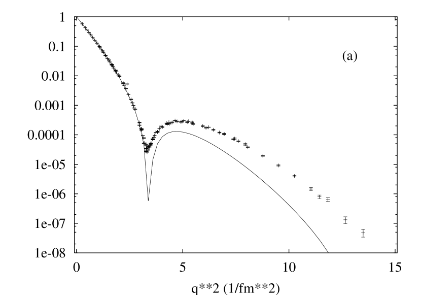
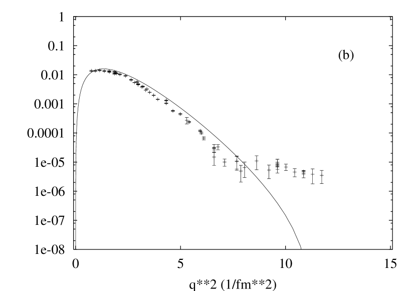
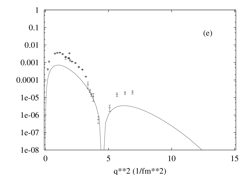
Figure 7: Comparison between the experimental form factors $|{\cal F}(0^{+}_{1}\rightarrow L^{P}_{i};q)|^{2}$ of ¹²C for the final states (a) $L^{P}_{i}=0^{+}_{1}$ (elastic), (b) $L^{P}_{i}=2^{+}_{1}$, (c) $L^{P}_{i}=3^{-}_{1}$, (d) $L^{P}_{i}=4^{+}_{1}$, (e) $L^{P}_{i}=0^{+}_{2}$, and (f) $L^{P}_{i}=1^{-}_{1}$ and those obtained for the oblate top with $N=10$.

Form factors for electron scattering on ¹²C have been measured in [10]-[17]. In Fig. 7 we show a comparison between experimental and theoretical form factors calculated in the oblate top limit of the ACM. The two coefficients that enter in the calculation of the theoretical form factors are determined by the minimum in the elastic form factor and the charge radius of ¹²C [5]. The analysis of the experimental form factors appears to indicate that the triangular configuration describes the data reasonably well for the rotational band $0_{1}^{+}$, $2_{1}^{+}$, $3_{1}^{-}$, $4_{1}^{+}$, although with large rotation-vibration interactions. The situation is different for the vibrational excitations $0_{2}^{+}$ and $1_{1}^{-}$. Here the shape of the form factors is well reproduced but its magnitude is not.

7 Summary and conclusions

In this contribution, we discussed cluster configurations consisting of three identical particles. These configurations are relevant for both hadronic physics (baryons as clusters of three constituent quarks), molecular physics (X₃ molecules) and nuclear physics (¹²C as a cluster of three $\alpha$ particles). It was suggested to treat the relative motion of the clusters in terms of the algebraic cluster model. The ACM is based on the algebraic quantization of the relative Jacobi variables which gives rise to a $U(7)$ spectrum generating algebra. We studied three special cases, for which the ACM provides a set of explicit formulas for energies, electromagnetic transition rates and form factors that can be easily be compared with experiments. In a semiclassical analysis it was shown that these three limits correspond to the spherical oscillator, the deformed oscillator and the oblate symmetric top.

The latter case, the oblate top, was applied to the low-lying states of ¹²C. In particular, we investigated the transition form factors. The shape of the form factors is reproduced reasonably well, lending support to the interpretation of the states of ¹²C as rotational and vibrational excitations of a triangular configuration of three $\alpha$ particles. However, the discrepancies with the observed strengths implies a large mixing with other configurations, and possibly the need to include higher order rotation-vibration couplings in the Hamiltonian.

Finally, we note that the ACM provides a general framework to study three-body clusters, which is not restricted to the case of three identical particles at the vertices of a triangle discussed in this contribution. It can be applied to other situations as well, such as nonidentical particles [18] and/or other geometrical configurations which may be relevant for a description of giant trinuclear molecules in ternary cold fission [4, 19].

References

• [1] F. Iachello and A. Arima, The Interacting Boson Model, (Cambridge University Press, 1987).
• [2] F. Iachello and R.D. Levine, Algebraic Theory of Molecules, (Oxford University Press, 1995).
• [3] R. Bijker, F. Iachello and A. Leviatan, Ann. Phys. (N.Y.) 236, 69 (1994).
• [4] Ş. Mişicu, P.O. Hess and W. Greiner, Phys. Rev. C 63, 054308 (2001).
• [5] R. Bijker and F. Iachello, Phys. Rev. C 61, 067305 (2000); Ann. Phys. (N.Y.) 298, 334 (2002).
• [6] O.S. van Roosmalen and A.E.L. Dieperink, Phys. Lett. B 100, 299 (1981); Ann. Phys. (N.Y.) 139, 198 (1982).
• [7] R.L. Hatch and S. Levit, Phys. Rev. C 25, 614 (1982); S. Levit and U. Smilansky, Nucl. Phys. A 389, 56 (1982).
• [8] R. Bijker and A. Leviatan, Rev. Mex. Fís. 44 S2, 15 (1998).
• [9] R. Bijker, A.E.L. Dieperink and A. Leviatan, Phys. Rev. A 52, 2786 (1995).
• [10] W. Reuter, G. Fricke, K. Merle and H. Miska, Phys. Rev. C 26, 806 (1982).
• [11] I. Sick and J.S. McCarthy, Nucl. Phys. A 150, 631 (1970).
• [12] H.L. Crannell and T.A. Griffy, Phys. Rev. 136, B1580 (1964).
• [13] H. Crannell, Phys. Rev. 148, 1107 (1966).
• [14] H. Crannell, J.T. O’Brien and D.I. Stober, in Int. Conf. on Nuclear Physics with Electromagnetic Interactions, (Mainz, 1979).
• [15] P. Strehl and Th.H. Schucan, Phys. Lett. 27B, 641 (1968).
• [16] Y. Torizuka, M. Oyamada, K. Nakahara, K. Sugiyama, Y. Kojima, T. Terasawa, K. Itoh, A. Yamaguchi and M. Kimura, Phys. Rev. Lett. 22, 544 (1969).
• [17] A. Nakada, Y. Torizuka and Y. Horikawa, Phys. Rev. Lett. 27, 745 and 1102 (1971).
• [18] R. Bijker and A. Leviatan, Few-Body Systems 25, 89 (1998).
• [19] R. Bijker, P.O. Hess and Ş. Mişicu, Heavy Ion Physics 13, 89 (2001);
P.O. Hess, R. Bijker and Ş. Mişicu, Rev. Mex. Fís. 47 S2, 52 (2001).