Geometry of random interactions

Abstract

It is argued that spectral features of quantal systems with random interactions can be given a geometric interpretation. This conjecture is investigated in the context of two simple models: a system of randomly interacting $d$ bosons and one of randomly interacting fermions in a $j={7\over 2}$ shell. In both examples the probability for a given state to become the ground state is shown to be related to a geometric property of a polygon or polyhedron which is entirely determined by particle number, shell size, and symmetry character of the states. Extensions to more general situations are discussed.

Recent studies in the nuclear shell model JON98 ; BIJ99 ; ZHA01 ; ZHA01b and the interacting boson model BIJ00 ; KUS00 with random interactions have unveiled a high degree of order. In particular, a marked statistical preference was found for ground states with $J=0^{+}$. In this Letter it is argued that spectral features of quantal systems with random interactions can be given a geometric interpretation which allows the computation of the probability for the quantum mechanical ground state to have a specific angular momentum, based on purely geometric considerations. Although these results are obtained in the context of a variety of simple models which do not cover the full complexity of random interactions, we believe them to be sufficiently general to conjecture the possibility of an entirely geometric analysis of the problem.

Consider a system consisting of $n$ interacting particles (bosons or fermions) carrying angular momentum $j$, integer or half-integer. Eigenstates of a rotationally invariant Hamiltonian are characterized as $|j^{n}\alpha JM\rangle$ where $J$ and $M$ are the total angular momentum and its projection, and $\alpha$ is any other index needed for a complete labeling of the state. Although spectral properties of a Hamiltonian with both one- and two-body interactions can be analyzed in the way explained below, we assume for simplicity that the one-body contribution is constant for all eigenenergies and that the energy spectrum is generated by two-body interactions only. Under this assumption its matrix elements can be written as

$$\langle j^{n}\alpha J|\hat{H}|j^{n}\alpha^{\prime}J\rangle={{n(n-1)}\over 2}\sum_{L}c^{L}_{n\alpha J}c^{L}_{n\alpha^{\prime}J}G_{L},$$ (1)

where $M$ is omitted since energies do not depend on it. The quantities $G_{L}$ are two-particle matrix elements, $G_{L}\equiv\langle j^{2}L|\hat{H}_{2}|j^{2}L\rangle$, and completely specify the two-body interaction while $c^{L}_{n\alpha J}$ are interaction-independent coefficients. They can be expressed in terms of coefficients of fractional parentage (CFP) TAL93 and, as such, are entirely determined by the symmetry character of the $n$-particle states.

We begin by considering the special case when a basis $|j^{n}\alpha JM\rangle$ can be found in which the expansion (1) is diagonal. In this case the Hamiltonian matrix elements reduce to the energy eigenvalues

$$E_{n\alpha J}={{n(n-1)}\over 2}\sum_{L}b^{L}_{n\alpha J}G_{L},$$ (2)

with $b^{L}_{n\alpha J}\equiv\left(c^{L}_{n\alpha J}\right)^{2}$. This is obviously a simplification of the more general problem (1) but nevertheless a wide variety of simple model situations can be accommodated by it. For example, this property is valid for any interaction between identical fermions if $j\leq{7\over 2}$ and remains so approximately for larger $j$ values; it is also exactly valid for $p$, $d$, or $f$ bosons. We shall refer to this class of problems as diagonal. For a constant interaction, $G_{L}=1$, all $n$-particle eigenstates are degenerate with energy ${1\over 2}n(n-1)$ and consequently the coefficients $b^{L}_{n\alpha J}$ satisfy the properties $\sum_{L}b^{L}_{n\alpha J}=1$ and $0\leq b^{L}_{n\alpha J}\leq 1$. Equation (2) can thus be rewritten in terms of scaled energies as

$$e_{n\alpha J}\equiv{{2E_{n\alpha J}}\over{n(n-1)}}=G_{L^{\prime}}+\sum_{L}b^{L}_{n\alpha J}(G_{L}-G_{L^{\prime}}),$$ (3)

for arbitrary $L^{\prime}$. This shows that, in the case of $N$ interaction matrix elements $G_{L}$, the energy of an arbitrary eigenstate can, up to a constant scale and shift, be represented as a point in a vector space spanned by $m\equiv N-1$ differences of matrix elements. Note that the position of these states is fixed by $b^{L}_{n\alpha J}$ and hence interaction-independent. Furthermore, since $0\leq b^{L}_{n\alpha J}\leq 1$, all states are confined to a compact region of this space with the size of one unit in each direction. For independent variables $G_{L}$ with covariance matrix $\langle G_{L}G_{L^{\prime}}\rangle=\delta_{LL^{\prime}}$, states are represented in an orthogonal basis. The differences in (3) are not independent but have a covariance matrix of the form $1+\delta_{LL^{\prime}}$; this leads to a representation in a $m$-simplex basis (i.e., an equilateral triangle in $m=2$ dimensions, a regular tetrahedron for $m=3$,…).

The following procedure can now be proposed to determine the probability $P_{n\alpha J}$ for a specific state $n\alpha J$ to become the ground state. First, construct all points corresponding to the energies $e_{n\alpha J}$. Next, build from them the largest possible convex polytope (i.e., convex polyhedron in $m$ dimensions). All points (i.e. states) inside this polytope can never be the ground state for whatever choice of matrix elements $G_{L}$ and thus have $P_{n\alpha J}=0$. Finally, the probability $P_{n\alpha J}$ of any other state at a vertex of the polytope is a function of some geometric property at that vertex.

This general procedure can be illustrated with some examples. Consider first a system of $j=2$ $d$ bosons. In this case there are three interaction matrix elements, $G_{0}$, $G_{2}$, and $G_{4}$ with $G_{L}\equiv\langle d^{2}L|\hat{H}_{2}|d^{2}L\rangle$; thus, $N=3$ and the problem can be represented in a plane. Because of the ${\rm U}(5)\supset{\rm SO}(5)\supset{\rm SO}(3)$ algebraic structure, an analytic solution is known for $n$ interacting $d$ bosons with eigenenergies BRI65 ; ARI76 ; CAS78

$$e_{n\tau J} = {{2n(n-2)+2\nu(\nu+3)-J(J+1)}\over{7n(n-1)}}(G_{2}-G_{4})$$ (4)

$$+ {{n(n+3)-\nu(\nu+3)}\over{5n(n-1)}}(G_{0}-G_{4})+G_{4},$$

where $\nu$ is the seniority quantum number which counts the number of $d$ bosons not in pairs coupled to angular momentum zero. Any energy $e_{n\nu J}$ can be represented as a point inside an equilateral triangle with vertices $G_{0}$, $G_{2}$, and $G_{4}$ of which the position is determined by the appropriate values on the edges $G_{0}-G_{4}$ and $G_{2}-G_{4}$. Examples for several boson numbers $n$ are shown in Fig. 1. For $n=2$ there are three states with $L=0,2,4$ and energies $e=G_{0},G_{2},G_{4}$; clearly, they have equal probability of being the ground state. As $n$ increases, more states appear in the triangle. The majority of states, shown as the smaller dots, are inside the convex polygon indicated in grey and can never be the ground state for whatever the choice of $G_{L}$.

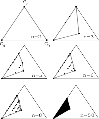
Figure 1: Polygons corresponding to several systems of interacting $d$ bosons. All states are represented by a dot. The smaller dots are inside or on the edge of a convex polygon (with the larger dots as vertices and indicated in grey) and are never the ground state. The probability of the vertex states to be the ground state is related to the angle at the vertex.

If we translate or rotate the convex polygon inside the triangle, its properties should not change since the points $G_{0}$, $G_{2}$, and $G_{4}$ are equivalent and since the distribution depends only on $\sum_{i}G_{i}^{2}$. Thus the probability for a point to be the ground state can only be related to the angle subtended at that vertex. The relation can be formally derived but also inferred from a few simple examples. If the polygon is an equilateral triangle, square, regular pentagon,…each vertex is equally probable with probability $1\over 3$, $1\over 4$, $1\over 5$,…One deduces the relation (see the $m=2$ polygons in Table 1)

$$P^{(2)}_{v}={1\over 2}-{{\theta_{v}}\over{2\pi}}$$ (5)

between the angle $\theta_{v}$ at the vertex $v$ of the polygon and the probability $P^{(2)}_{v}$ for the state associated with that vertex to be the ground state.

Table 1: The angle or the angle sum $\sum_{f\ni v}\theta_{vf}$ and the vertex probability $P_{v}$ of regular polygons ($m=2$) and polyhedrons ($m=3$).

	$m$	$\displaystyle{\sum_{f\ni v}\theta_{vf}}$	$P_{v}$		$m$	$\displaystyle{\sum_{f\ni v}\theta_{vf}}$	$P_{v}$
triangle	2	${1\over 3}\pi$	$1\over 3$	tetrahedron	3	$\pi$	$1\over 4$
square	2	${1\over 2}\pi$	$1\over 4$	octahedron	3	${4\over 3}\pi$	$1\over 6$
pentagon	2	${3\over 5}\pi$	$1\over 5$	icosahedron	3	${5\over 3}\pi$	$1\over{12}$
hexagon	2	${2\over 3}\pi$	$1\over 6$	cube	3	${3\over 2}\pi$	$1\over 8$
$p$-gon	2	${{p-2}\over p}\pi$	$1\over p$	dodecahedron	3	${9\over 5}\pi$	$1\over{20}$

Table 2 compares probabilities calculated with the analytic relation (5) with those obtained from numerical tests for several systems of randomly interacting $d$ bosons with boson numbers $n=5,6,10,18$. The numerical probabilities are obtained from 20000 runs with random interaction parameters. They agree with the analytic result (5).

Table 2: Probabilities $P_{n\nu J}$ (in %) of some $d$-boson states obtained analytically with formula (5) and numerically with Gaussian parameters.

		Probability $P_{n\nu J}$				Probability $P_{n\nu J}$
$n$	$J(\nu)$	Analytic	Gaussian	$n$	$J(\nu)$	Analytic	Gaussian
5	0(3)	4.08	3.96	10	0(0)	20.87	20.77
	2(1)	20.11	19.96		0(6)	0.50	0.41
	2(5)	36.19	36.59		0(10)	37.56	37.96
	10(5)	39.63	39.49		10(10)	41.08	40.85
6	0(0)	22.32	22.13	18	0(0)	19.89	19.87
	0(6)	38.05	38.37		0(18)	37.56	38.37
	12(6)	39.63	39.49		36(18)	42.06	41.75

A second example concerns a system of four $j={7\over 2}$ fermions which was discussed recently by Zhao and Arima ZHA01 . In this case there are four interaction matrix elements, $G_{0}$, $G_{2}$, $G_{4}$, $G_{6}$ with $G_{L}\equiv\langle j^{2}L|\hat{H}_{2}|j^{2}L\rangle$, and this leads to a problem that can be represented in three-dimensional space. Any state in the $j={7\over 2}$ shell can be labeled with particle number $n$, seniority $\nu$, and total angular momentum $J$ with analytically known expansion coefficients $b^{L}_{n\nu J}$ TAL93 . For $n=4$ there are eight different states and the corresponding coefficients $b^{L}_{n\nu J}$ are given in Ref. ZHA01 . These eight states can be represented in three-dimensional space spanned by the three differences $G_{0}-G_{6}$, $G_{2}-G_{6}$, and $G_{4}-G_{6}$, and six of them define a convex polyhedron (see Fig. 2). The two remaining points [corresponding to the state $J(\nu)=4(2)$ and 5(4)] are inside this polyhedron and are never the ground state. The relation between the geometry of the polyhedron and the probability $P^{(3)}_{v}$ of each vertex state to be the ground state can again be inferred from a few simple examples.

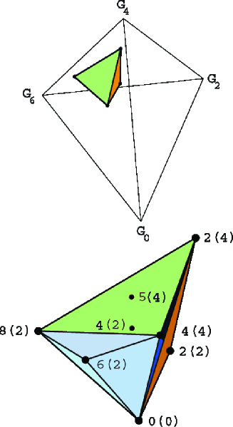
Figure 2: The polyhedron for a system of $n=4$ $j={7\over 2}$ fermions. The upper part indicates the position of the polyhedron in the tetrahedral coordinate system. The left part shows the same (enlarged) polyhedron with vertices that correspond to the states $J(\nu)$ that can become the ground state with a probability given by the exterior angle. Two additional states with $J(\nu)=4(2)$ and 5(4) lie inside or on the face of the polyhedron and are never the ground state. For representation purposes the polyhedral face 0(0)–2(4)–8(2) has been removed in the left part.

The relevant quantity in this case is $\sum_{f\ni v}\theta_{vf}$ where the sum is over all faces that contain the vertex $v$ and $\theta_{vf}$ is the angle at vertex $v$ in face $f$. A few examples with regular polyhedrons (see the $m=3$ polyhedrons in Table 1) demonstrate that the relation is

$$P^{(3)}_{v}={1\over 2}-{1\over{4\pi}}\sum_{f\ni v}\theta_{vf}.$$ (6)

Table 3 compares the probabilities for the different states to become the ground state as calculated in various approaches. The second column gives the analytic results obtained from (6) while the third column lists numerical results obtained from 20000 runs with random matrix elements with a Gaussian distribution. As our code does not distinguish between states with the same angular momentum $J$ but different seniority $\nu$, only the summed probability for each $J$ is given. The last column shows the results of Zhao and Arima ZHA01 who calculate the probability as a multiple integral.

Table 3: Probabilities $P_{n\nu J}$ (in %) of $n=4$ $j={7\over 2}$ states obtained with the analytic formula (6), from a numerical calculation, and from the integral representation of Zhao and Arima ZHA01 .

	Probability $P_{n\nu J}$
$J(\nu)$	Analytic	Numerical	Integral
0(0)	18.33	18.38	18.19
2(2)	1.06	—	0.89
2(4)	33.22	—	33.25
2(2&4)	34.28	34.88	34.14
4(2)	0	—	0.00
4(4)	23.17	—	22.96
4(2&4)	23.17	22.83	22.96
5(4)	0	0.00	0.00
6(2)	0.05	0.07	0.02
8(2)	24.16	23.83	24.15

These notions can be generalized in several ways. The first is towards energies that depend on a set of continuous variables $\{t_{1},\dots,t_{q}\}$ as follows [compare with Eq. (2)]:

$$E(t_{1},\dots,t_{q})=\sum_{L}b_{L}(t_{1},\dots,t_{q})G_{L}.$$ (7)

The analogous problem now consists in the determination of the probability density $dP(t_{1},\dots,t_{q})$ for obtaining the lowest energy at $\{t_{1},\dots,t_{q}\}$ with random interactions $G_{L}$. We assume by way of example that the number of variables $q$ is one less than the number $N$ of interactions $G_{L}$, $q=N-1$. In that case Eq. (7) represents a $q$-dimensional hypersurface $\Sigma^{q}$ embedded in a $(q+1)$-dimensional Euclidean space E^q+1 (the metric follows from the covariance matrix $\langle G_{L}G_{L^{\prime}}\rangle=\delta_{LL^{\prime}}$). Let us suppose that $\Sigma^{q}$ is the closed orientable manifold. It can then be shown that the probability density is given by Gauss’ spherical map KoNo69 $\Sigma^{q}\to S^{q}$ where $S^{q}$ is a $q$-dimensional hypersphere of a unit radius. If the degree of the spherical map is one (as it is for closed convex surfaces), the probability density reads

$$dP(t_{1},\dots,t_{q})={\frac{1}{S_{q}}}K_{q}(t_{1},\dots,t_{q})dv,$$ (8)

where $K_{q}$ is the Gaussian curvature of $\Sigma^{q}$, $S_{q}$ is the volume of the unit hypersphere $S^{q}$ and $dv$ denotes an infinitesimal element of $\Sigma^{q}$. In the simplest example of one parameter $t_{1}\equiv t$ and two interactions $G_{1}$ and $G_{2}$, the energy is parametrized as a curve in a plane. It can then be shown that the probability density is given by $dP(t)=(2\pi)^{-1}K_{1}(t)ds$, where $ds$ is the infinitesimal arc length. In fact, this formula is also valid for piecewise curves and precisely leads to the result (5) for a polygon. The validity of the result can be checked by comparing the probability obtained by integration of (8) over a part of $\Sigma^{q}$ to the numerically calculated one. As an example we discuss a two-dimensional ellipsoid in E³ with one semi-axis $c$ different from the others $a$. The probability associated with the part of the surface with spherical coordinates $(\theta,\phi)$ satisfying $0\leq\theta\leq\theta_{0}$ and $0\leq\phi\leq\phi_{0}$ is given by

$$P(\theta_{0},\phi_{0})=\frac{\theta_{0}}{4\pi}\left(1-\frac{a\cos\phi_{0}}{\sqrt{c^{2}+(a^{2}-c^{2})(\cos{\phi_{0}})^{2}}}\right).$$ (9)

This expression has been compared with the numerically calculated probability; the difference is close to zero. We have analyzed likewise the case of a three-dimensional hyperellipsoid in E⁴, showing that our approach can be generalized to higher dimensions. These results also open up the possibility for an extension to higher-dimensional polytopes, by replacing the right-hand side of (Eq. 8) with an appropriate characteristic for each vertex of the polytope. Indeed, it can be shown that the probabilities $P^{(m)}_{v}$ in (5) and (6) are related to the exterior angle at vertex $v$ GRU67 ; BAN67 of either a convex polygon ($m=2$) or a convex polyhedron ($m=3$).

We believe that, although derived for a restricted form of interaction Hamiltonians, these results suggest that generic $n$-body quantum systems, interacting through two-body forces, can be associated with a geometrical shape defined in terms of CFPs or generalized coupling coefficients. Geometry thus arises as a consequence of strong correlations implicit in such systems and is independent of particular two-body interactions. Random tests can be understood in this context as sampling experiments on this geometry. In this Letter we have shown that geometric aspects of $n$-body systems determine some of their essential characteristics. In particular, for diagonal Hamiltonians surface curvature defines probability to be the ground state. Other correlations could also be related to geometric features. These results generalize and put onto a firm basis the previous work which hinted at a purely geometric interpretation of randomly interacting boson systems BIJ00 ; KUS00 , as well as provide an explanation for the method of Zhao and collaborators ZHA01 . In fact, in the latter reference, the authors have advanced some qualitative reasons for certain states to dominate and later provided an approximate procedure (which is not always accurate ZHA02 ) to estimate the ground state probabilities, although no reason was offered for its success. Our study, at least for the case where the Hamiltonian is diagonal, clearly shows that the procedure of Zhao et al is equivalent to a projection of the considered above polyhedra on the axes defined by the two-body matrix elements, which tend to correlate well with the angles we introduce. This connection will be elaborated in detail elsewhere CHAU . Further work is required to fully explore the geometry and its consequences for our understanding of $n$-body dynamics.

Acknowledgments: AF is supported by CONACyT, Mexico, under project 32397-E. NAS thanks L. Vanhecke for a helpful discussion.

References

-
(1)
C.W. Johnson, G.F. Bertsch, and D.J. Dean,
Phys. Rev. Lett. 80, 2749 (1998);
C.W. Johnson et al., Phys. Rev. C 61, 014311 (2000). -
(2)
R. Bijker, A. Frank, and S. Pittel,
Phys. Rev. C 60, 021302 (1999);
V. Velazquez and A.P. Zuker, Phys. Rev. Lett. 88, 072502 (2002). - (3) Y.M. Zhao and A. Arima, Phys. Rev. C 64, 041301 (2001).
-
(4)
Y.M. Zhao, A. Arima, and N. Yoshinaga,
Phys. Rev. C 66, 034302 (2002);
D.M. Mulhall, A. Volya, and V. Zelevinsky, Phys. Rev. Lett. 85, 4016 (2000). - (5) R. Bijker and A. Frank, Phys. Rev. Lett. 84, 420 (2000); Phys. Rev. C 64, 061303 (2001); Nucl. Phys. News Vol 11, 20 (2001).
-
(6)
D. Kusnezov,
Phys. Rev. Lett. 85, 3773 (2000);
L.F. Santos, D. Kusnezov, and Ph. Jacquod, nucl-th/0201049. - (7) I. Talmi, Simple Models of Complex Nuclei (Harwood, Chur, Switzerland, 1993).
- (8) D.M. Brink, A.F.R. De Toledo Piza, and A.K. Kerman, Phys. Lett. 19, 413 (1965).
- (9) A. Arima and F. Iachello, Ann. Phys. (NY) 99, 253 (1976).
- (10) O. Castaños, A. Frank, and M. Moshinsky, J. Math. Phys. 19, 1781 (1978).
- (11) Sh. Kobayashi and K. Nomizu, Foundations of Differential Geometry (Wiley, New York, 1969).
- (12) B. Grünbaum, Convex Polytopes (Wiley, New York, 1967).
- (13) T. Banchoff, J. Diff. Geom. 1, 245 (1967).
- (14) Y.M. Zhao, A. Arima, and N. Yoshinaga, nucl-th/0206040.
- (15) P.H.-T.Chau et al (in preparation).