The role of E1-E2 interplay in multiphonon Coulomb excitation

Abstract

In this work we study the problem of a charged particle, bound in a harmonic-oscillator potential, being excited by the Coulomb field from a fast charged projectile. Based on a classical solution to the problem and using the squeezed-state formalism we are able to treat exactly both dipole and quadrupole Coulomb field components. Addressing various transition amplitudes and processes of multiphonon excitation we study different aspects resulting from the interplay between E1 and E2 fields, ranging from classical dynamic polarization effects to questions of quantum interference. We compare exact calculations with approximate methods. Results of this work and the formalism we present can be useful in studies of nuclear reaction physics and in atomic stopping theory.

I Introduction

Recent studies of Coulomb-induced breakup of weakly bound nuclei indicate a considerable reduction of the dissociation probability in comparison with the prediction of the first-order Born calculation Esbensen and Bertsch (2002). The reduction is associated with dynamic polarization, where the quadrupole field creates a polarization that influences the effects induced by the dominating electric dipole. This is a well-known phenomenon in atomic stopping theory, where the stopping power for charged particles deviates from the $Z^{2}$ dependence of Bethe’s formula Bethe (1930), $Z$ being the charge of a particle. Measurements, as for example, of the stopping power for protons and anti-protons Andersen et al. (1989), indicate the presence of a $Z^{3}$ correction. Over the years a substantial progress has been made in measuring and understanding of this phenomenon Andersen (1983); Porter and Jeppesen (1983); Porter and Lin (1990); Novkovic et al. (1993); Pitarke et al. (1993); Arista and Lifschitz (1999); Leung (1989).

In this work we consider the Coulomb excitation of a charged particle bound by a harmonic-oscillator potential. The time-dependent electric dipole (E1) and quadrupole (E2) fields of a projectile excite the particle, and within this approximation the quantum problem is treated exactly. This problem has been studied in the past, starting from the classical treatment by Ashley, Ritchie, and Brandt Ashley et al. (1972), followed by quantum perturbation theory Hill and Merzbacher (1974), and later further perturbative Born terms Mikkelsen and Sigmund (1989); Mikkelsen and Flyvbjerg (1990) have also been considered. Exact numerical solutions to the time-dependent quantum problem have been demonstrated by Mikkelsen and Flyvbjerg Mikkelsen and Flyvbjerg (1992). The use of a harmonic oscillator model, as was previously argued Mikkelsen and Sigmund (1989), is justified for reasons of simplicity and at the same time good quality of results in comparison with observed stopping powers. The preset work adds yet another reason, as it demonstrates how classical results such as Ashley et al. (1972); Jackson and McCarthy (1972) can be used to obtain exact quantum answers. Thus, the approach presented here does not involve heavy numerical calculations. It presents a simple and transparent way to understand and to treat exactly the Coulomb excitation of an oscillator. As an application of the presented technique, rather than repeating previous numerical calculations, we concentrate on a less explored aspect of Coulomb excitation; here the overall excitation probability, the dipole and quadrupole transition amplitudes, and their interplay are discussed.

We use a connection between classical and quantum mechanics which is usually complex and in most cases takes an approximate quasiclassical form. However, in situations where the dynamics of a system is determined by linear equations of motion, with arbitrary time-dependent parameters, the classical-to-quantum correspondence is exact. The harmonic oscillator which is driven by the time-dependence of its parameters, such as mass, frequency or external force, is an example of such a situation. Most theoretical developments in the field of parametric excitations of harmonic systems were done more than three decades ago Lewis (1967); Lewis and Riesenfeld (1969); Popov and Perelomov (1969, 1970); Baz et al. (1969). Despite this, it is only during the past decade theorists began to embrace the beauty of this problem and to discuss its relevance to many physical processes. Photon generation, lasers Abdalla et al. (1998), quantum interference and two-photon excitations Georgiades et al. (1999), phase transitions, critical phenomena Isar (1999); Drummond et al. (2001), information theory Aliaga et al. (1993), ion traps, oriented chiral condensates Volya et al. (2000) are examples of recent developments. Squeezed states that appear as solutions in parametrically driven harmonic systems, also known as two-photon coherent states, generalize the concept of coherent states Glauber (1963) to include two-quanta couplings in the radiation field Yuen (1976); Hartley and Ray (1982).

By presenting this work we further expand applications of the squeezed state formalism to problems of Coulomb excitation. We focus our efforts on classical and quantum effects resulting from the interplay of one-(dipole) and two-quanta (quadrupole) couplings of an oscillator system to an external field. Using symmetries we derive simple formulas for excitation probabilities and transition amplitudes that explicitly show quantum interference effects and can be used to improve perturbative calculations.

This work is divided into four sections. In Sec. II we review the properties of harmonic-oscillator systems and the transition from a classical to a quantum description, which is based on canonical transformation. We summarize the properties of the parameters that describe the initial state to final state transition ($S$-matrix) and derive transition amplitudes and excitation probability relevant to Coulomb excitation. Section III is dedicated to applications. Here we consider the classical solution and address the transition to the quantum treatment. We discuss quantum corrections, perturbative limits, charge asymmetry, and two-phonon excitations. The role of E1 and E2 interplay is emphasized in these discussions. We summarize our findings in Sec. IV.

II Parametric excitation of coupled oscillator system

We consider a system of $N$ oscillators with the unperturbed Hamiltonian

$$H_{0}=\sum_{l}\left(\frac{p_{l}^{2}}{2}+\frac{\omega_{l}^{2}\,q_{l}^{2}}{2}\right)\,.$$ (1)

These oscillators are disturbed by a time-dependent force $F_{l}(t)$ and time-dependent frequency parameters $Q_{l\,l^{\prime}}(t)=Q_{l^{\prime}\,l}(t)\,,$ expressed by

$$H_{\rm int}(t)=\frac{1}{2}\sum_{l\,l^{\prime}}\,Q_{l\,l^{\prime}}(t)q_{l}q_{l^{\prime}}+\sum_{l}F_{l}(t)q_{l}\,.$$ (2)

It is assumed that $H_{\rm int}(t)=0$ in the infinite past $t\rightarrow-\infty$ and in the infinite future $t\rightarrow\infty\,.$ First we quantize this problem in the infinite past. Here

$$q_{l}=\frac{1}{\sqrt{2\omega_{l}}}\left(a_{l}e^{-i\omega_{l}t}+a_{l}^{\dagger}e^{i\omega_{l}t}\right)\,,$$ (3a)

$$p_{l}=-i\sqrt{\frac{\omega_{l}}{2}}\left(a_{l}e^{-i\omega_{l}t}-a^{\dagger}_{l}e^{i\omega_{l}t}\right)\,,$$ (3b)

where $a^{\dagger}_{l}$ and $a_{l}$ are time-independent creation and annihilation operators for the $l$-th mode. For any other time we introduce creation and annihilation operators $b^{\dagger}_{l}(t)$ and $b_{l}(t)$ so that the coordinates and momenta in the Heisenberg representation are

$$q_{l}=\frac{1}{\sqrt{2\omega_{l}}}\left(b_{l}(t)e^{-i\omega_{l}t}+b^{\dagger}_{l}(t)e^{i\omega_{l}t}\right)\,,$$ (4a)

$$p_{l}=-i\sqrt{\frac{\omega_{l}}{2}}\left(b_{l}(t)e^{-i\omega_{l}t}-b^{\dagger}_{l}(t)e^{i\omega_{l}t}\right)\,.$$ (4b)

The operators $b^{\dagger}(t)$ and $b(t)$ are defined in the interaction representation, as the time dependence due to $H_{0}$ is introduced explicitly in Eq. (4). For the infinite past we have by definition

$$b(-\infty)=a\,,\quad b^{\dagger}(-\infty)=a^{\dagger}\,.$$ (5)

At $t\rightarrow+\infty\,$ $b(t)$ and $b^{\dagger}(t)$ also become time-independent

$$b(\infty)=b\,,\quad b^{\dagger}(\infty)=b^{\dagger}\,.$$ (6)

The transformation from the original operators $a$ and $a^{\dagger}$ to the intermediate $b$ and $b^{\dagger}$ is determined by a general Bogoliubov transformation

$$b_{l}(t)=\sum_{l^{\prime}}\left(u_{l\,l^{\prime}}(t)a_{l^{\prime}}+v_{l\,l^{\prime}}(t)a^{\dagger}_{l^{\prime}}\right)+c_{l}(t)\,.$$ (7)

In order to simplify the notation we will write this in matrix form as

$$b(t)=u(t)a+v(t)a^{\dagger}+c(t)\,.$$ (8)

The perturbation $H_{\rm int}$ drives the nontrivial time dependence of these creation and annihilation operators

$$i\frac{d}{dt}b=[b(t),\,H_{\rm int}]={\cal F}(t)+{\cal Q}^{-}(t)b+{\cal Q}^{+}(t)b^{\dagger}\,,$$ (9)

where matrices

$${{\cal Q}^{\pm}}_{l\,l^{\prime}}(t)=\frac{Q_{l\,l^{\prime}}(t)}{2\sqrt{\omega_{l}\,\omega_{l^{\prime}}}}\,e^{i(\omega_{l}\pm\omega_{l^{\prime}})t}\,$$ (10)

and a vector

$${\cal F}_{l}(t)=\frac{F_{l}(t)}{\sqrt{2\omega_{l}}}\,e^{i\omega_{l}t}\,$$

are introduced. The ${{\cal Q}^{-}}$ and ${{\cal Q}^{+}}$ are hermitian and symmetric matrices, respectively. The time dependence of the parameters $u$ and $v\,,$ as follows from (9), are determined from

$$i\frac{d}{dt}\,u={{\cal Q}^{-}}\,u+{{\cal Q}^{+}}\,v^{*}\,,$$ (11a)

$$i\frac{d}{dt}\,v={{\cal Q}^{-}}\,v+{{\cal Q}^{+}}\,u^{*}\,,$$ (11b)

and

$$i\frac{d}{dt}\,c={{\cal Q}^{-}}\,c+{{\cal Q}^{+}}\,c^{*}+{\cal F}\,.$$ (12)

These equations are solved numerically with initial conditions

$$u(-\infty)=1\,,\quad v(-\infty)=0\,,\quad c(-\infty)=0\,,$$ (13)

which follow from (5). We stress here that solving Eqs. (11) and (12) is equivalent to finding a full classical solution to the problem. This follows from the fact that the equations of motion are linear, so the time-dependence of a Heisenberg operator becomes identical to the time-dependence of its classical analog.

II.1 Properties of the $S$-matrix

In this work we will be interested only in the initial to final state transition probabilities, i.e., in the $S$ matrix that comes from the transformation of operators

$$b=ua+va^{\dagger}+c\,,\quad b^{\dagger}=u^{*}a^{\dagger}+v^{*}a+c^{*}\,.$$ (14)

The inverse transformation is

$$a=u^{\dagger}b-v^{T}b^{\dagger}+c^{\prime}\,,\quad a^{\dagger}=u^{T}b^{\dagger}-v^{\dagger}+{c^{\prime}}^{*}\,,$$ (15)

where

$$c^{\prime}=-u^{\dagger}c+v^{T}c^{*}\,.$$ (16)

Transformation (14) is canonical and preserves commutation relations so that if $[a_{l},\,a^{\dagger}_{l^{\prime}}]=\delta_{l\,l^{\prime}}$ then $[b_{l},\,b^{\dagger}_{l^{\prime}}]=\delta_{l\,l^{\prime}}\,;$ this puts some conditions on the matrices $u$ and $v$

$$uu^{\dagger}-vv^{\dagger}=1\,,\quad uv^{T}-vu^{T}=0\,,$$ (17a)

$$uu^{\dagger}-v^{T}v^{*}=1\,,\quad u^{\dagger}v-v^{T}u^{*}=0\,.$$ (17b)

These linear canonical transformations, so-called symplectic transformations, are often encountered in classical mechanics. The generators of the above symplectic transformation form a group which generalizes the simple $SU(1,1)\,$ group Profilo and Soliana (1991); Gerry (1987); Lianfu et al. (1997) of a one-dimensional oscillator. In general any infinitesimal time evolution can be described by a linear canonical transformation which preserves the phase space in accordance with Liouville’s theorem. The beauty of our case is that the linearity remains for any period of time evolution. This allows for an exact classical-to-quantum correspondence. Besides the method that we implement in this paper, the Wigner transformation Wigner (1932) that establishes the correspondence between the classical phase space distribution and the quantum density matrix can also be used to exactly reconstruct the quantum solution from its classical analog Esbensen (1981). The application of the Wigner transformation in studies of various properties of the harmonic oscillator has been demonstrated repeatedly Han et al. (1988); Agarwal and Arun Kumar (1991); Aliaga et al. (1993).

II.2 Survival probability

Here we assume that $u\,,$ $v$ and $c\,$ are known. Using these we determine transition amplitudes between quantum states. Coherent states,

$$|\alpha\rangle=e^{-|\alpha|^{2}/2}\sum_{n=0}^{\infty}\frac{\alpha^{n}}{\sqrt{n!}}\,|n\rangle\,,$$ (18)

provide the best means for addressing this problem. In this basis the evolution operator $U$ is Mollow (1967)

$$\langle\beta|U|\alpha\rangle=A^{0}\exp\left(-\frac{1}{2}(|\beta^{2}|+|\alpha^{2}|)+\frac{1}{2}\beta^{\dagger}v(u^{*})^{-1}\beta^{*}-\frac{1}{2}\alpha^{T}(u^{*})^{-1}v\alpha+\beta^{\dagger}(u^{\dagger})^{-1}\alpha-\beta^{\dagger}(u^{\dagger})^{-1}c^{\prime}-\alpha^{T}(u^{*})^{-1}c^{*}\right)\,.$$ (19)

The normalization constant $A^{0}$ is determined by the completeness condition

$$\frac{1}{\pi^{N}}\int d^{2N}\beta\,|\langle\beta|U|\alpha\rangle|^{2}=1\,,$$ (20)

where integration goes through both real and imaginary parts of $\beta\,.$ This is an important parameter, since it sets the scale of all transitions and it determines the probability to remain in the ground state $P_{0,0}=|\langle 0|U|0\rangle|^{2}={|A^{0}|}^{2}\,.$ The quantity $P_{0,0}$ is given by the Gaussian integral, where $\alpha$ is set to zero for simplicity

$$\frac{\pi^{N}}{P_{0,0}}=\int d^{2N}\beta\exp\left\{-|\beta|^{2}+\Re(\beta^{T}\rho\beta+2c^{T}\beta-2c^{\dagger}\rho\beta)\right\}\,.$$ (21)

We introduce here the matrix

$$\rho=v(u^{*})^{-1}\,,$$ (22)

which is a characteristic of quadrupole excitation. Besides some trivial normalization that will be further discussed, the matrix element $\rho_{i\,j}$ is the amplitude of a single step two-quanta excitation of $i$-th and $j$-th modes. The classical time evolution of this matrix follows from the time evolution of $u$ and $v$ (11), and is given by

$$i\frac{d}{dt}\rho=\rho{{\cal Q}^{-}}^{*}+{{\cal Q}^{-}}\rho+\rho{{\cal Q}^{+}}^{*}\rho+{{\cal Q}^{+}}\,.$$ (23)

This result explicitly shows that $\rho$ is a symmetric matrix ($\rho=\rho^{T}$).

The multidimensional Gaussian integral can be taken as

$$\int d^{2n}{\bf b}\exp(-{\bf b}^{T}{\bf A}{\bf b}+2{\bf s}^{T}{\bf b})=\frac{\pi^{n}}{\sqrt{\det{\bf A}}}\exp\left({\bf s}^{T}{\bf A}^{-1}{\bf s}\right)\,,$$ (24)

where relevant to our case

$${\bf b}=\left(\begin{array}[]{c}\Re{\beta}\\ \Im{\beta}\end{array}\right)\,,\quad{\bf c}=\left(\begin{array}[]{c}\Re{c}\\ \Im{c}\end{array}\right)\,,\,{\bf A}=\left(\begin{array}[]{cc}1-\Re\rho&\Im\rho\\ \Im\rho&1+\Re\rho\end{array}\right),$$ (25)

$${\bf s}={\bf Q}^{T}{\bf c}\,,\quad{\bf Q}=\left(\begin{array}[]{cc}1-\Re\rho&\Im\rho\\ -\Im\rho&-(1+\Re\rho)\end{array}\right)\,.$$ (26)

Because of the previously discussed properties of the Bogoliubov transformation, inversion of the matrix ${\bf A}$ is not needed. It can be shown that $-{\bf c}^{T}{\bf Q}{\bf A}^{-1}{\bf Q}^{T}{\bf c}=-{c}^{\dagger}{c}+\Re(c^{T}\rho^{*}c)\,.$ This results in

$$P_{00}=\sqrt{\det(1-\rho^{\dagger}\rho)}\,\,\exp\left[-{c}^{\dagger}{c}+\Re(c^{T}\rho^{*}c)\right]\,.$$ (27)

The survival probability in the above form unifies the roles of E1 and E2 processes, and establishes a direct and simple relation between the quantities of perturbation theory, $\rho$ and $c\,,$ and the exact answer. There is a clear meaning of the different terms in the product (27). The $\exp({-c^{\dagger}c})$ represents the excitation of a coherent state due to the dipole interaction; the term $\sqrt{\det(1-\rho^{\dagger}\rho)}$ is a result of quadrupole squeezing Volya et al. (2000). The remaining part $\exp[\Re(c^{T}\rho^{*}c)]$ is a result of quantum interference.

II.3 Transition Amplitudes

Equation (19) can be used to obtain transition amplitudes. Coefficients in a Taylor expansion of (19) are related to transition amplitudes between oscillator states Volya et al. (2000), with one-dimensional oscillator, for example,

$$\langle\beta|U|\alpha\rangle=e^{-(|\alpha|^{2}+|\beta|^{2})/2}\,\sum_{n,m}\langle n|U|m\rangle\frac{(\beta^{*})^{n}\alpha^{m}}{\sqrt{n!m!}}\,.$$ (28)

Below we denote by $|i,j,k\dots\rangle$ the normalized state containing single quanta in $i,j,k\dots\,$ oscillator modes (later we will use directions $x\,$ $y$ and $z$). A single-quantum excitation amplitude is given by

$$\langle j|U|0\rangle=-A^{0}\{(u^{\dagger})^{-1}c^{\prime}\}_{j}=A^{0}\{(c-\rho c^{*})\}_{j}\,,$$ (29)

where the subscript $j$ denotes a component of the vector in the brackets. Since the interaction vanishes in both the infinite past and infinite future, the transition probabilities are symmetric with respect to initial and final states, in agreement with general principles of quantum mechanics. However, the decay amplitude from an excited one-phonon state to the ground state, which is

$$\langle 0|U|j\rangle=-A^{0}\{(u^{*})^{-1}c^{*}\}_{j}\,,$$ (30)

differs from the excitation amplitude by a non trivial phase. This emphasizes the effect of quantum interference between dipole and quadrupole amplitudes. Setting either $c$ or $\rho$ to zero restores the symmetry.

The transition amplitude from the ground state to the excited state with two oscillator quanta, requires expansion of (19) to the order $\beta^{2}$

$$\langle ij|U|0\rangle=\frac{\sqrt{1+\delta_{ij}}}{2}\left(A^{0}\rho_{ij}+\frac{\langle i|U|0\rangle\langle j|U|0\rangle}{A^{0}}\right)\,.$$ (31)

The first term in the above equation is due to a direct quadrupole transition, since its amplitude is directly proportional to $\rho\,.$ The second term describes the second-order dipole process.

For an initially excited system the transition amplitudes can be calculated in a similar manner, by expanding in both $\alpha$ and $\beta\,;$ for example

$$\langle i|U|j\rangle=A^{0}(u^{\dagger})^{-1}_{ij}+\frac{\langle i|U|0\rangle\langle 0|U|j\rangle}{A^{0}}\,.$$ (32)

Tailor expansion of a Gaussian form can be used to define Hermite polynomials, in particular for the multi-variable case such as Eq. (19). This, in turn, allows for an analytic expression of transition amplitudes between oscillator states. Useful iterative relations between amplitudes that follow from properties of Hermite polynomials can be obtained in this way, or alternatively, iterative relations can be derived directly from the properties of the evolution operator Fernandez and Tipping (1989).

The energy transfer, which is important for calculating the stopping power, can be calculated using Eq. (14). For the excitation from the ground state we obtain

$$\Delta E=\langle 0|\sum_{l}\omega_{l}b^{\dagger}_{l}b_{l}|0\rangle=\sum_{l}\omega_{l}|c_{l}|^{2}+\sum_{ll^{\prime}}\omega_{l}|v_{ll^{\prime}}|^{2}\,.$$ (33)

The above presents an average energy transfer. The energy spread can also be calculated as in Volya et al. (2000).

II.4 One dimensional harmonic oscillator

The special case of a one-dimensional harmonic oscillator with time-dependent parameters has been extensively studied previously Husimi (1953); Popov and Perelomov (1969, 1970); Baz et al. (1969); Sebawe Abdalla (1986a, b); Abe and Ehrhardt (1993). According to Eq. (27) the probability to remain in the ground state is

$$P_{00}=\sqrt{1-|\rho|^{2}}\,\,\exp\left\{-|c|^{2}\left[1-|\rho|\cos(\phi_{\rho}-2\phi_{c})\right]\right\}\,,$$ (34)

where $\phi_{\rho}$ and $\phi_{c}$ are phases of $\rho$ and $c\,,$ respectively. This agrees with the previously obtained result Baz et al. (1969). We will further on encounter a one-dimensional case where $c=0\,.$ Here only even-quanta transitions are possible, and the excitation probabilities from the ground state and first excited state by $2n$ quanta are

$$P_{0,2n}=\frac{(2n)!}{2^{2n}(n!)^{2}}\,|\rho|^{2n}\,\sqrt{1-|\rho|^{2}}\,,$$ (35)

$$P_{1,2n+1}=\frac{(2n+1)!}{2^{2n}(n!)^{2}}\,|\rho|^{2n}\,(1-|\rho|^{2})^{3/2}\,.$$ (36)

III Coulomb excitation

We consider here the problem of Coulomb excitation of a particle bound in a harmonic-oscillator potential, by a projectile of charge $Z$. We assume that the projectile moves along a fixed trajectory ${\vec{R}}(t)\,$ in the $xy$ plane. In order to utilize the treatment discussed above we expand the Coulomb potential up to quadratic terms in the particle coordinate $q\,,$ namely, treating it in the dipole-quadrupole approximation

$$V_{\rm coul}(t)=\frac{C}{R^{3}}\,{\vec{q}}\cdot{\vec{R}}+\frac{C}{2R^{5}}\left(3({\vec{q}}\cdot{\vec{R}})^{2}-q^{2}R^{2}\right)\,,$$ (37)

where $C=Ze^{2}\,.$ The non-zero components of $H_{\rm int}$ defined in Eq. (2) are

$$F_{x}(t)=\frac{CR_{x}}{R^{3}}\,,\quad F_{y}(t)=\frac{CR_{y}}{R^{3}}\,,$$ (38)

$$Q_{xx}=\frac{C}{R^{5}}\left(3R_{x}^{2}-R^{2}\right)\,\quad Q_{yy}=\frac{C}{R^{5}}\left(3R_{y}^{2}-R^{2}\right)\,,$$

$$Q_{xy}=Q_{yx}=\frac{3CR_{x}R_{y}}{R^{5}}\,,\quad Q_{zz}=-\frac{C}{R^{3}}\,.$$ (39)

These expressions show that the mode in the direction perpendicular to the scattering plane is decoupled, and it is excited by the quadrupole term only. Further, we assume a straight line trajectory so that ${\vec{R}}(t)=(b,\,{\rm v}t,\,0)\,.$ This does not simplify the problem, since our formalism can be used for any trajectory. This assumption, however, allows us to compare with previous results Ashley et al. (1972); Hill and Merzbacher (1974); Mikkelsen and Sigmund (1989). We introduce the following notations

$${\mathfrak{d}}_{i}=\frac{C}{b{\rm v}\sqrt{2\omega_{i}}}\,,\quad{\mathfrak{q}}_{ij}=\frac{C}{2b^{2}{\rm v}\,\sqrt{\omega_{i}\omega_{j}}}\,,$$ (40)

and

$$\xi_{i}=\frac{b\omega_{i}}{{\rm v}}\,,$$ (41)

where $i$ and $j$ are indices referring to $x\,,$ $y$ and $z\,$ directions. Often we will assume $\omega_{x}=\omega_{y}=\omega_{z}=\omega\,;$ in that case the corresponding indices are omitted. The parameters ${\mathfrak{d}}$ and ${\mathfrak{q}}$ can be viewed as dipole and quadrupole strengths, so that their ratio $1/(b\sqrt{2\omega})$ determines the applicability of the multipole expansion.

III.1 Perturbative treatment

Here we will discuss several approximations. The first one is the usual approximation relevant to multipole expansion of the Coulomb field. It utilizes the smallness of the photon wave length as compared to the size of the system. The next two limits are the “sudden limit” where $\xi\ll 1$ and the “adiabatic limit” $\xi\gg 1\,.$ Finally, we will use the term Born approximation which corresponds to some order in the iterative solution of the classical equations (11) and (12). Since the classical equations of motion allow here for an exact reconstruction of the wave function, the use of this terminology does not contradict its quantum notion.

All of the results in this study, such as in Eqs. (27), (29), and (31), are fully determined by the parameters $c$ and $\rho\,,$ which may be referred to as shift (dipole) and squeezing (quadrupole) parameters, respectively. Both of these parameters can be expanded using the above approximations. Each order of Born approximation results in the next order correction in terms of the quadrupole strength (40). Thus an expansion of $c$ and $\rho$ is a series

$$c={\mathfrak{d}}\sum_{n=1,2,\dots}{\mathfrak{c}}^{(n)}(\xi){\mathfrak{q}}^{n-1}\,,\quad\rho=\sum_{n=1,2,\dots}{\mathfrak{r}}^{(n)}(\xi){\mathfrak{q}}^{n}\,,$$ (42)

where $n=1,2\dots\,$ is the corresponding Born order. The coefficients ${\mathfrak{c}}^{(n)}$ and ${\mathfrak{r}}^{(n)}$ are $\xi$ dependent only.

The lowest order long-range dipole approximation is a textbooks example Bertulani and Baur (1988). Using Eq. (12) we obtain

$$c\approx{\mathfrak{d}}\,c^{(1)}=\int_{-\infty}^{\infty}\,-i\,\frac{F_{l}(t)}{\sqrt{2\omega_{l}}}\,e^{i\omega_{l}t}\,dt\,.$$ (43)

This leads to

$$c^{(1)}_{x}=-2i\xi_{x}K_{1}\left(\xi_{x}\right)\,,\quad c^{(1)}_{y}=2\xi_{y}K_{0}\left(\xi_{y}\right)\,,\quad c^{(1)}_{z}=0\,.$$ (44)

We note that $c^{(1)}_{y}$ is real, and $c^{(1)}_{x}$ is imaginary.

Using (23) the squeezing parameter $\rho$ can be calculated in a similar Born-type perturbative manner. In the lowest order we obtain

$$\rho_{xx}=-4i{\mathfrak{q}}_{xx}\,\xi_{x}\left[K_{1}(2\xi_{x})+2\xi K_{0}(2\xi_{x})\right]\,,$$ (45a)

$$\rho_{yy}=8i{\mathfrak{q}}_{yy}\,\xi_{y}^{2}K_{0}(2\xi_{y})\,,$$ (45b)

$$\rho_{xy}=4{\mathfrak{q}}_{xy}\,\sqrt{\xi_{x}\xi_{y}}\,(\xi_{x}+\xi_{y})\,K_{1}(\xi_{x}+\xi_{y})\,,$$ (45c)

$$\rho_{zz}=4i{\mathfrak{q}}_{zz}\,\xi_{z}K_{1}(2\xi_{z})\,.$$ (45d)

The above results can also be obtained using time dependent perturbation theory. The first order excitation probability in the $i$-th direction is $P^{{\rm I}}_{i}=|c_{i}|^{2}\,.$ The probability to excite quanta $i,j$ in a single step quadrupole process is to the lowest order $P^{{\rm II}}_{i,j}=(1+\delta_{i,j})|\rho_{ij}|^{2}/4\,.$ These results can be compared with the exact transition amplitudes in Eqs. (29) and (31).

In the sudden limit $\xi\rightarrow 0$ the dipole contribution comes from the transverse direction: $c_{x}\approx-2i{\mathfrak{d}}\,,$ while for quadrupole excitations $|\rho_{xx}|\approx|\rho_{zz}|\approx 2{\mathfrak{q}}\,$ are dominant in this limit. The adiabatic limit $\xi\rightarrow\infty$ is a textbook example of preservation of adiabatic invariances with exponential precision Landau and Lifshitz (1976).

III.2 $Z^{3}$ corrections in classical solutions

The long range dipole contribution is the main part of the cross section, thus any corrections to $c$ are the most important. We denote as $c_{0}(t)$ the inhomogeneous part of the solution to Eq. (12)

$$c_{0}(t)=-i\int_{-\infty}^{t}{\cal F}(t^{\prime})dt^{\prime}\,.$$ (46)

The $c_{0}\equiv c_{0}(\infty)=dc^{(1)}$ is the previously discussed first Born dipole amplitude. The second Born correction, which here simply means the second order approximation to the classical solution of Eq. (12) is

$$i\delta c=\int_{-\infty}^{\infty}[{{\cal Q}^{-}}c_{0}(t)+{{\cal Q}^{+}}c^{*}_{0}(t)]dt\,.$$ (47)

This integral can be studied numerically or perturbatively with respect to $\xi\,.$

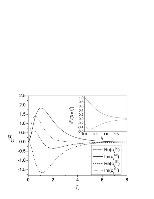
Figure 1: The lowest order polarization corrections to the dipole amplitude are plotted as a function of $\xi\,.$ The insert shows the behavior of $\Im(c^{(2)}_{x})$ and $\Re(c^{(2)}_{y})$ relative to $3\pi\xi^{2}\,.$

In Fig. 1 the dependence of the real and imaginary parts of $c$ are shown as functions of $\xi\,.$ In the adiabatic limit, which corresponds to large $\xi$ all of these functions decay exponentially: $c^{(2)}\sim\exp(-2\xi)$ as dictated by the adiabatic nature Landau and Lifshitz (1976). Approaching the sudden limit all corrections go to zero as powers of $\xi\,.$ In the $\xi\rightarrow 0$ limit $\Im{\mathfrak{c}}^{(1)}_{x}$ is the dominant term, and the lowest order correction to it is $\Im{\mathfrak{c}}^{(2)}_{x}\approx 3\pi\xi^{2}\,.$ This leads to the following approximation for the probability Ashley et al. (1972)

$$P_{\rm x}=4{\mathfrak{d}}^{2}(1-3\pi\mathfrak{q}\xi^{2})\,.$$ (48)

The above correction behaves as $Z^{3}$ with the charge of the projectile, and reduces the excitation probability in repulsive Coulomb scattering. This correction is completely classical as it appears in a solution of classical differential equations, see Ashley et al. (1972). Note that the homogeneous part of (12) which is the source of this polarization effect, is caused by the E2 field.

Higher order corrections to the squeezing parameter $\rho\,$ are relatively large but are generally less important due to the overall smallness of the quadrupole amplitude. Here again we iteratively solve the classical equation (23). This equation contains no dipole parameters, thus the correction on $\rho$ is self-induced and would not change in the absence of the E1 field. Assuming that

$$i\rho_{0}(t)=\int_{-\infty}^{t}{{\cal Q}^{+}}(t^{\prime})dt^{\prime}=\int_{-\infty}^{\infty}dt^{\prime}\Theta(t-t^{\prime})\,{{\cal Q}^{+}}(t^{\prime})\,,$$ (49)

the second Born correction is

$$i\delta\rho=\int_{-\infty}^{\infty}dt\left(\rho_{0}(t){{\cal Q}^{-}}(t)+{{\cal Q}^{-}}^{*}(t)\rho_{0}(t)\right)\,.$$ (50)

For the case of equal frequencies, this expression can be calculated analytically

$$\delta\rho_{xx}=8{\mathfrak{q}}^{2}\xi\left[K_{1}(2\xi)-2\xi K_{2}(2\xi)\right]-i\pi{\mathfrak{q}}^{2}\xi(1-2\xi)e^{-2\xi}\,,\quad$$ (51a)

$$\delta\rho_{xy}=-2\pi{\mathfrak{q}}^{2}\xi^{2}e^{-2\xi}-8i{\mathfrak{q}}^{2}\xi^{2}K_{1}(2\xi)\,,\qquad$$ (51b)

$$\delta\rho_{yy}=-i\pi{\mathfrak{q}}^{2}\xi(1+2\xi)e^{-2\xi}\,,\qquad$$ (51c)

$$\delta\rho_{zz}=-8{\mathfrak{q}}^{2}\xi K_{1}(2\xi)+\frac{16}{3}i{\mathfrak{q}}^{2}\xi^{2}K_{1}(2\xi)\,.\qquad$$ (51d)

In the $\xi\rightarrow 0$ limit, excitations due to the quadrupole field comes from the $x$ and $z$ directions, leading to the following approximate E2 contribution to the excitation probability

$$\Delta P_{\rho}=2{\mathfrak{q}}^{2}(1+\pi{\mathfrak{q}}\xi(1-4\xi))+2{\mathfrak{q}}^{2}\left(1+\frac{8}{3}{\mathfrak{q}}\xi\right)\,.$$ (52)

The charge asymmetry in this case is of opposite sign, resulting in an enhanced probability for repulsive interaction. This enhancement can only be observed in measurements if the dominant dipole transitions are blocked or restricted.

III.3 Exact treatment

We start this section by showing the comparison of the exact excitation probability and the first Born dipole approximation, $P_{\rm born}=c_{0}^{\dagger}c_{0}\,,$ see Fig. 2. The harmonic-oscillator model is rather crude and can not be used to fully understand features of the realistic Coulomb dissociation of nuclei. However, it can still provide a qualitative picture. For example the Coulomb dissociation of ${}^{17}_{9}$F can be looked at assuming that the proton outside the oxygen core is bound by a harmonic potential. The frequency of the oscillator, related to the dipole excitation energy, is assumed to be of the order of 1 MeV. In this case a unit of the oscillator length corresponds to 6.4 fm. Assuming Coulomb excitation by ${}^{56}_{28}$Ni we have $C=6.3\,.$ The choice of parameters used in some figures below is guided by this model. In Fig. 2 we use impact parameter $b=4\,$ ($b=25.6$ fm), $C=6\,,$ and the range of velocities from 0.2 to 20 (oscillator units) that corresponds to the incident energies from 0.02 to 200 MeV/u. The choice of impact parameter is restricted by the range of applicability of the multipole expansion $\sqrt{2}b\gg 1\,.$ Our discussions also imply that the probability to find the nucleon in the oscillator at a distance from origin larger than impact parameter is negligible. For $b=2$ this probability is 4%, assuming the ground state wave function. However for $b=4$ that we use, this is less than $10^{-3}$ %.

As seen in Fig. 2 the effects of higher order corrections are significant. The a difference between repulsive and attractive interactions is also transparent. This confirms the recent results of more realistic calculations Esbensen and Bertsch (2002).

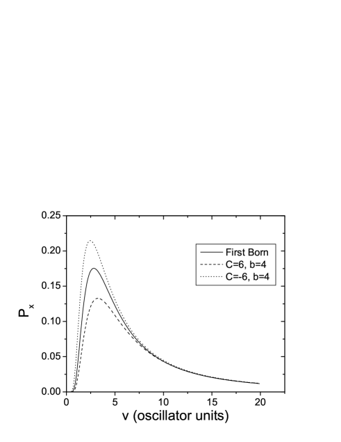
Figure 2: Excitation probability as a function of incident velocity, at the impact parameter $b=4\,.$ The dashed line is the result of the repulsive interaction, $C=6\,.$ The dotted line corresponds to the attractive interaction $C=-6\,.$ These results are compared to the first Born dipole approximation shown by the solid line.

III.3.1 Higher-order corrections

From the classical solutions for $\rho$ and $c$ exact quantum results can be extracted using Eq. (27). In order to discuss the impact of a quantum treatment we can make an expansion of the exact answer in Eq. (27), which gives

$$P_{\rm x}=1-P_{00}\approx c^{\dagger}c-\frac{(c^{\dagger}c)^{2}}{2}+\frac{1}{2}{\rm Tr}(\rho^{\dagger}\rho)-\Re(c^{T}\rho^{*}c)\,$$ (53)

$$=P_{\rm born}+\Delta P_{c}+\Delta P_{\rho}+\Delta P_{\rm inter}\,.$$

We identify here three main corrections to the first Born dipole excitation probability. The first is

$$\Delta P_{c}=c^{\dagger}c-\frac{(c^{\dagger}c)^{2}}{2}-P_{\rm born}\,,$$

which is a correction to the dipole transition probability. It is known that the excitation of a quantum oscillator by an external force creates a coherent state. The dipole amplitude $c\,,$ which is related to a classical shift of the oscillator from its equilibrium position, appears in the exponent of Eq. (27). This accounts for all second and higher order E1 processes. Exponentiation of the dipole amplitude, in order to account for the loss of strength to multi-phonon excitations, has been previously discussed Norbury and Baur (1993). We stress here that other parts of $\Delta P_{c}\,$ are of classical origin and mainly $Z^{3}$-dependent. They come from the effect of the quadrupole field on the shift of the oscillator from its equilibrium. This creates a deviation of $c$ from the Born result $c_{0}$ as discussed in Sec. III.2.

The next term in (53),

$$\Delta P_{\rho}={\rm Tr}(\rho^{\dagger}\rho)/2\,,$$

is a quadrupole contribution, which comes from the expansion of the square root in (27). Similar to the exponent in the dipole term, the use of the square root accounts for all higher order quadrupole transitions.

Finally, a very interesting and purely quantum interference effect appears through the last term in (53),

$$\Delta P_{\rm inter}=-\Re(c^{T}\rho^{*}c)\,.$$

Although it may seem that this is a quantum Barkas correction, correction vanishes to lowest order. This follows from Eqs. (44) and (45).

In Fig. 3 the absolute values of $\Delta P_{c}\,,$ $\Delta P_{\rho}\,,$ and $\Delta P_{\rm inter}$ relative to the first Born E1 probability are plotted as functions of velocity.

Figure 3: Corrections to the first Born E1 probability. Values are relative to $P_{\rm born}$. Logarithmic scale is used to show contributions of very different magnitude. Corrections $\Delta P_{c}/P_{\rm born}$ $\Delta P_{\rho}/P_{\rm born}$ and $\Delta P_{\rm inter}/P_{\rm born}$ are shown in dotted, dashed and solid lines, respectively. Parameters $b=4$ and $C=6\,$ are used for this figure.

The figure demonstrates that dominant corrections to the first order dipole probability come from second and higher order dipole transitions, and from the lowest order quadrupole. The interference term contributes only on the level of 1%, and quickly vanishes in the sudden limit. As discussed above, the interference term vanishes to order $Z^{3}\,.$ Thus it is a $Z^{4}$ term to leading order.

III.3.2 $Z$-dependence

In order to examine the $Z$-odd part of the excitation probability from a different point of view we introduce the Barkas factor

$$B=\frac{P_{\rm x}(Z)-P_{\rm x}(-Z)}{P_{\rm x}(Z)+P_{\rm x}(-Z)}\,.$$ (54)

As discussed above this effect owes its existence to the classical dynamic interplay between E1 and E2 fields. With the validity of a multipole expansion, the bulk of this correction is expected to be proportional to the quadrupole amplitude ${\mathfrak{q}}\,.$ In Fig. 4 $B/{\mathfrak{q}}$ is plotted as a function of $\xi\,.$

Figure 4: The Barkas factor as a function of $\xi\,,$ for various parameters. The classical correction to the sudden limit, $3\pi\xi^{2}\,,$ is shown by a dashed curve.

Various cases corresponding to different impact parameters and projectile charges are considered. In the second Born approximation, the $B/{\mathfrak{q}}$ is only a function of $\xi\,,$ thus independent of both charge and impact parameter Mikkelsen and Sigmund (1989). Deviations observed on the plot emphasize the significance of other corrections that scale as higher powers in ${\mathfrak{q}}$ and higher odd powers in $Z\,.$

The charge asymmetry related to the dipole-quadrupole interference appears naturally in various transition amplitudes. The Fig. 5 shows the transition probability from the ground state to the state with two quanta in $z$ direction. In this transition the vanishing out-of-plane dipole force makes the quadrupole term dominant. As demonstrated by Eq. (52) the $Z^{3}$ Barkas-type charge dependence of the quadrupole term $\rho$ is of the opposite sign in comparison to the dipole-quadrupole case shown in Figs. 2 and 4. In agreement with this, an enhancement of the excitation probability in repulsive Coulomb interaction is observed in Fig. 5.

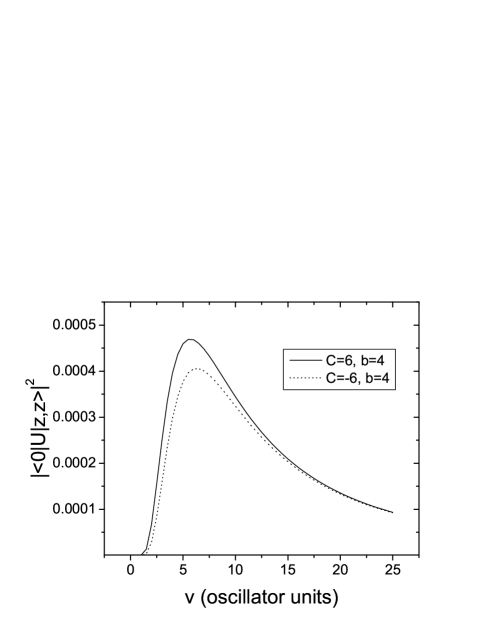
Figure 5: The transition probability from the ground state to the two-quantum excitated state in the $z$ direction is shown as a function of incident velocity. Solid and dotted lines correspond to repulsive and attractive Coulomb force, respectively.

III.3.3 Interplay of dipole and quadrupole fields

Our harmonic-oscillator model incorporates E1 and E2 electromagnetic processes exactly. The role and interplay of these processes in multi-phonon excitation may be of interest in the physics of Giant Dipole Resonances (GDR) Bertulani et al. (1996); Norbury and Baur (1993). Although precise calculations with inclusion of the relevant microscopic physics of GDR are beyond the scope of this paper, we consider here the effect that the E2 process plays in the two phonon excitation probability

$$P_{0,2}=\sum_{i<j}|\langle ij|U|0\rangle|^{2}\,.$$

We introduce a quadrupole coupling strength $x$ which simply scales the quadrupole part of the perturbation Hamiltonian (2). This can be viewed as scaling the quadrupole strength ${\mathfrak{q}}\rightarrow x{\mathfrak{q}}\,.$ The limits $x=0$ and $x=1$ naturally correspond to the cases when E2 is neglected and when E2 is at its natural value, respectively. Eq. (31), as one would expect from perturbation theory, shows that the amplitude for a two-phonon excitation is given by the sum of two terms that reflect the first order quadrupole and second order dipole processes. The E1 and E2 interplay is not trivial here and comes in several places. The first term in (31) at large quadruple strength is directly proportional to $x\,.$ Thus in this limit a quadratic scaling of the excitation amplitude is expected. At a smaller strength a substantial contribution to the second term in (31) appears as a classical dynamic polarization effect, influencing the amplitude $c\,.$ This can reduce the excitation probability for a repulsive interaction. Finally, the phases of terms in (31) can interfere. It must be noted that the dynamic polarization disappears at very low and very high velocities. Also both ${\mathfrak{d}}\sim 1/v$ and ${\mathfrak{q}}\sim 1/v$ but since dipole comes in the second order, the quadrupole amplitude dominates at high velocity leading to

$$P_{0,2}(x)=4{\mathfrak{q}}^{2}x^{2}\,.$$ (55)

In Fig. 6 the two-phonon excitation probability as a function of the coupling strength $x$ is shown relative to the case with no E2, $x=0\,.$ Observed features are in agreement with the above discussion. Cases corresponding to repulsive interaction, shown by solid lines, always lead to reduced probability as compared to kinematically identical situations but attractive interaction (dashed lines). The dynamic polarization effect is maximized around $v=3$ which is consistent with the enhanced charge asymmetry observed in Fig. 2. In this velocity regime, the polarization effect is so strong that for repulsive interactions “turning on” the quadrupole field ($x=1$) leads to a reduction of a two-phonon excitation probability.

Figure 6: Relative two-phonon excitation probability as a function of the quadrupole strength.

IV Conclusions

In this work we considered a simple model of a charged particle in a harmonic-oscillator potential. The system is excited by the electric dipole and quadrupole fields of a charged projectile passing by. We have developed an application of the squeezed-state formalism to solve this problem exactly. In terms of the one-phonon dipole excitation amplitudes $c$ and the direct two-phonon quadrupole excitation amplitudes $\rho\,$ we derived simple expressions for various transition amplitudes, and the total and multi-phonon excitation probabilities. The parameters $c$ and $\rho$ are determined from classical equations. Our results are exact for a harmonic oscillator. For a general case they can be used as a parameterization, extending the higher-order (multi-phonon) dipole approximation introduced by Norbury and Baur Norbury and Baur (1993) to include the quadrupole field and related interference effects.

We discussed the interplay between the electric dipole and quadrupole fields and the resulting effects on various excitation probabilities. In the intermediate range of energies, between instant and adiabatic limits, ($0.5<\xi<7$) the influence of dynamic polarization dominates. It was shown that the origin of this effect is purely classical. The quadrupole polarization influences the effect of the dipole force, leading to a significant change in the excitation probability. This phenomenon, known in stopping power theory as Barkas effect, in the lowest order leads to a $Z^{3}$ charge dependence, and reduces the excitation probability for repulsive Coulomb interactions. We found a similar classical effect of self-induced polarization in the quadrupole amplitude. This effect is of the opposite sign and for the same repulsive kinematics results in an enhancement of the quadrupole amplitude. The effect was demonstrated in $z$-polarized two-phonon excitations. Our exact results exhibit some additional higher-order quantum contributions, but corrections from these are small. We presented a number of numerical calculations and plots that demonstrate a variety of observable phenomena that can be attributed to the E1-E2 interplay.

By presenting this work we hope to introduce the coherent plus squeezed-state formalism to the field of nuclear reaction physics and nuclear excitations. Numerous developments that use dipole excitations can be extended to include quadrupole transitions. Not every physical situation can be described by a harmonic oscillator. However, armed with an exact solution and a full set of time-dependent wave functions, perturbation theory based on squeezed states can be a promising future direction.