Concerning the quark condensate

Abstract

A continuum expression for the trace of the massive dressed-quark propagator is used to explicate a connection between the infrared limit of the QCD Dirac operator’s spectrum and the quark condensate appearing in the operator product expansion, and the connection is verified via comparison with a lattice-QCD simulation. The pseudoscalar vacuum polarisation provides a good approximation to the condensate over a larger range of current-quark masses.

I Introduction

Dynamical chiral symmetry breaking (DCSB) is a cornerstone of hadron physics. This phenomenon whereby, even in the absence of a current-quark mass, self-interactions generate a momentum-dependent running quark mass, $M(p^{2})$, that is large in the infrared: $M(0)\sim 0.5\,$GeV, but power-law suppressed in the ultraviolet masslessuv :

$$M(p^{2})\stackrel{{\scriptstyle{\rm large}-p^{2}}}{{=}}\,\frac{2\pi^{2}\gamma_{m}}{3}\,\frac{\left(-\,\langle\bar{q}q\rangle^{0}\right)}{p^{2}\left(\frac{1}{2}\ln\left[\frac{p^{2}}{\Lambda_{\rm QCD}^{2}}\right]\right)^{1-\gamma_{m}}}\,,$$ (1)

is impossible in weakly interacting theories. In Eq. (1), $\gamma_{m}=12/(33-2N_{f})$ is the mass anomalous dimension, with $N_{f}$ the number of light-quark flavours, and $\langle\bar{q}q\rangle^{0}$ is the renormalisation-group-invariant vacuum quark condensate mr97 , to which we shall hereafter refer as the OPE condensate. While Eq. (1) is expressed in Landau gauge, $\langle\bar{q}q\rangle^{0}$ is gauge parameter independent. In the chiral limit the OPE condensate plays a role analogous to that played by the renormalisation-group-invariant current-quark mass in the massive theory: it sets the scale of the mass function in the ultraviolet.

The evolution of the dressed-quark mass-function in Eq. (1) to a large and finite constituent-quark-like mass in the infrared, $M(0)\sim 0.5\,$GeV, is a longstanding prediction of Dyson-Schwinger equation (DSE) studies cdragw that has recently been confirmed in simulations of quenched lattice-QCD latticequark . A determination of the OPE condensate directly from lattice-QCD simulations must await an accurate chiral extrapolation latticequarkchiral but DSE models tuned to reproduce modern lattice data give pmqnp2002 $(-\langle\bar{q}q\rangle^{0})\sim\Lambda_{\rm QCD}^{3}$.

Another view of DCSB is obtained by considering the eigenvalues and eigenfunctions of the massless Euclidean Dirac operator fn:Eucl :

$$\gamma\cdot D\,u_{n}(x)=i\lambda_{n}\,u_{n}(x)\,.$$ (2)

The operator is anti-Hermitian and hence the eigenfunctions form a complete set, and except for zero modes they occur in pairs: $\{u_{n}(x),\gamma_{5}u_{n}(x)\}$, with eigenvalues of opposite sign. It follows that in an external gauge field, $A$, one can write the Green function for a massive propagating quark in the form

$$S(x,y;A)=\langle q(x)\bar{q}(y)\rangle_{A}=\sum_{n}\frac{u_{n}(x)\,u_{n}^{\dagger}(y)}{i\lambda_{n}+m}\,,$$ (3)

where $m$ is the current-quark mass and, naturally, the eigenvalues depend on $A$. (NB. The expectation value denotes a Grassmannian functional integral evaluated with a fixed gauge field configuration.) Assuming, e.g., a lattice regularisation, it follows that

$$\frac{1}{V}\,\int_{V}d^{4}x\,\langle\bar{q}(x)q(x)\rangle_{A}=-\frac{2m}{V}\,\sum_{\lambda_{n}>0}\,\frac{1}{\lambda_{n}^{2}+m^{2}}\,,$$ (4)

where $V$ is the lattice volume fn:zero . One may now define a quark condensate as the infinite volume limit of the average in Eq. (4) over all gauge field configurations:

$$\langle 0|\bar{q}q|0\rangle:=\lim_{V\to\infty}\frac{1}{V}\,\int_{V}d^{4}x\,\left\langle\,\langle\bar{q}(x)q(x)\rangle_{A}\,\right\rangle\,.$$ (5)

In the infinite volume limit the operator spectrum becomes dense and Eqs. (4), (5) become

$$-\langle 0|\bar{q}q|0\rangle=2m\int_{0}^{\infty}d\lambda\,\frac{\rho(\lambda)}{\lambda^{2}+m^{2}}\,,$$ (6)

with $\rho(\lambda)$ the spectral density. This equation expresses an assumption that in QCD the full two-point massive-quark Schwinger function, when viewed as a function of the current-quark mass, has a spectral representation.

It follows formally from Eq. (6) that

$$\lim_{m\to 0}\,m\int_{0}^{\infty}d\lambda\,\frac{\rho(\lambda)}{\lambda^{2}+m^{2}}=\frac{1}{2}\,\pi\,\rho(0)\,,$$ (7)

and hence one arrives at the chiral limit result

$$-\langle 0|\bar{q}q|0\rangle=\pi\,\rho(0)\,.$$ (8)

This is the so-called Banks-Casher relation bankscasher ; Marinari . It has long been advocated as a means by which a quark condensate may be measured in lattice-QCD simulations Marinari and has been used in analysing chiral symmetry restoration at nonzero temperature Harald and chemical potential Harald2 , and to explore the connection between magnetic monopoles and chiral symmetry breaking in $U(1)$ gauge theory simon . Much has been learnt verbaarschot ; Jacextras by exploiting the fact that qualitative features of the behaviour of $\rho(\lambda)$ for $\lambda\sim 0$ can be understood using chiral random matrix theory; i.e., from considerations based solely on QCD’s global symmetries.

Our main goal is to explicate a correspondence between the condensate in Eq. (1) and that in Eq. (8). In Sec. II we discuss the OPE condensate and its connection with QCD’s gap equation, and emphasise that the residue of the lowest-mass pole-contribution to the flavour-nonsinglet pseudoscalar vacuum polarisation is a direct measure of the OPE condensate mrt98 . A natural ability to express DCSB through the formation of a nonzero OPE condensate is fundamental to the success of DSE models of hadron phenomena reviews . In Sec. III we carefully define the trace of the massive dressed-quark propagator and use that to illustrate a connection between $\rho(0)$ and the OPE condensate, which we verify via comparison with a lattice simulation. Section IV is an epilogue.

II OPE Condensate

II.1 Gap and Bethe-Salpeter equations

Dynamical chiral symmetry breaking in QCD is readily explored using the DSE for the quark self-energy:

$$S(p)^{-1}=Z_{2}\,(i\gamma\cdot p+m^{\rm bm})$$ (9)

$$+\,Z_{1}\int^{\Lambda}_{q}\,g^{2}D_{\mu\nu}(p-q)\frac{\lambda^{a}}{2}\gamma_{\mu}S(q)\Gamma^{a}_{\nu}(q,p)\,,$$

wherein: $D_{\mu\nu}(k)$ is the renormalised dressed-gluon propagator; $\Gamma^{a}_{\nu}(q;p)$ is the renormalised dressed-quark-gluon vertex; $m^{\rm bm}$ is the $\Lambda$-dependent current-quark bare mass that appears in the Lagrangian; and $\int^{\Lambda}_{q}:=\int^{\Lambda}d^{4}q/(2\pi)^{4}$ represents a translationally-invariant regularisation of the integral, with $\Lambda$ the regularisation mass-scale which is removed to infinity as the completion of all calculations. The quark-gluon-vertex and quark wave function renormalisation constants, $Z_{1}(\zeta^{2},\Lambda^{2})$ and $Z_{2}(\zeta^{2},\Lambda^{2})$ respectively, depend on the renormalisation point, the regularisation mass-scale and the gauge parameter.

If the current-quark mass changes with flavour, then the solution of Eq. (9) is flavour dependent:

$$S_{f}(p)^{-1} = i\gamma\cdot p\,A_{f}(p^{2},\zeta^{2})+B_{f}(p^{2},\zeta^{2})$$ (10)

$$= \frac{1}{Z_{f}(p^{2},\zeta^{2})}\left[i\gamma\cdot p+M_{f}(p^{2},\zeta^{2})\right]\,,$$

and is obtained subject to the condition that at some large, spacelike $\zeta^{2}$

$$\left.S_{f}(p)^{-1}\right|_{p^{2}=\zeta^{2}}=i\gamma\cdot p+m_{f}(\zeta)\,,$$ (11)

where $m_{f}(\zeta)$ is the renormalised current-quark mass:

$$Z_{4}(\zeta,\Lambda)\,m_{f}(\zeta)=Z_{2}(\zeta,\Lambda)\,m_{f}^{\rm bm}(\Lambda)\,,$$ (12)

with $Z_{4}$ the renormalisation constant for the scalar part of the quark self-energy. Since QCD is an asymptotically free theory, the chiral limit is defined by

$$Z_{2}(\zeta^{2},\Lambda^{2})\,m_{f}^{\rm bm}(\Lambda)\equiv 0\,,\;\;\Lambda\gg\zeta$$ (13)

and in this case the scalar projection of Eq. (9) does not exhibit an ultraviolet divergence mrt98 ; mr97 .

Important in describing chiral symmetry is the axial-vector Ward-Takahashi identity:

$$P_{\mu}\Gamma_{5\mu}^{H}(k;P) = {\cal S}^{-1}(k_{+})\,i\gamma_{5}\frac{T^{H}}{2}+i\gamma_{5}\frac{T^{H}}{2}{\cal S}^{-1}(k_{-})$$

$$-M_{(\zeta)}\,i\Gamma_{5}^{H}(k;P)-i\Gamma_{5}^{H}(k;P)\,M_{(\zeta)}\,,$$

where $P$ is the total momentum entering the vertex. In Eq. (LABEL:avwti): $M_{(\zeta)}={\rm diag}[m_{u}(\zeta),m_{d}(\zeta),m_{s}(\zeta)]$, ${\cal S}={\rm diag}[S_{u},S_{d},S_{s}]$ and $\{T^{H}\}$ are flavour matrices, e.g., $T^{\pi^{+}}=\frac{1}{2}\left(\lambda^{1}+i\lambda^{2}\right)$ (we consider SU${}_{f}(3)$ because chiral symmetry is unimportant for heavier quarks); $\Gamma_{5\mu}^{H}(k;P)$ is the renormalised axial-vector vertex, which is obtained from the inhomogeneous Bethe-Salpeter equation

$$\left[\Gamma_{5\mu}^{H}(k;P)\right]_{tu}=Z_{2}\,\left[\gamma_{5}\gamma_{\mu}\frac{T^{H}}{2}\right]_{tu}$$ (15)

$$+ \int^{\Lambda}_{q}\,[\chi_{5\mu}^{H}(q;P)]_{sr}\,K^{rs}_{tu}(q,k;P)\,,$$

where $\chi_{5\mu}^{H}:={\cal S}(q_{+})\Gamma_{5\mu}^{H}(q;P){\cal S}(q_{-})$, $q_{\pm}=q\pm P/2$, and $K(q,k;P)$ is the fully renormalised quark-antiquark scattering kernel; and $\Gamma_{5}^{H}$ is the pseudoscalar vertex,

$$\left[\Gamma_{5}^{H}(k;P)\right]_{tu}=Z_{4}\,\left[\gamma_{5}\frac{T^{H}}{2}\right]_{tu}$$ (16)

$$+ \int^{\Lambda}_{q}\,\left[\chi_{5}^{H}(q;P)\right]_{sr}K^{rs}_{tu}(q,k;P)\,,$$

with $\chi_{5}^{H}:={\cal S}(q_{+})\Gamma_{5}^{H}(q;P){\cal S}(q_{-})$. Multiplicative renormalisability ensures that no new renormalisation constants appear in Eqs. (15) and (16).

Flavour-octet pseudoscalar bound states appear as coincident pole solutions of Eqs. (15), (16), namely,

$$\Gamma_{5\mu}^{H}(k;P)\propto\Gamma_{5}^{H}(k;P)\propto\frac{1}{P^{2}+m_{H}^{2}}\,\Gamma_{H}(k;P)\,,$$ (17)

where $\Gamma_{H}$ is the bound state’s Bethe-Salpeter amplitude and $m_{H}$, its mass. (Regular terms are overwhelmed at the pole.) Consequently, Eq. (LABEL:avwti) entails mrt98 ; mr97

$$f_{H}\,m_{H}^{2}=r_{H}^{(\zeta)}\,{\cal M}_{H}^{(\zeta)}\,,$$ (18)

where: ${\cal M}_{H}^{(\zeta)}={\rm tr}_{\rm flavour}[M_{(\zeta)}\{T^{H},(T^{H})^{\rm t}]$ is the sum of the constituents’ current-quark masses (“t” denotes matrix transpose); and

$$f_{H}P_{\mu} = Z_{2}\int^{\Lambda}_{q}\,\frac{1}{2}{\rm tr}\left[\left(T^{H}\right)^{\rm t}\gamma_{5}\gamma_{\mu}\chi_{H}(q;P)\right]\,,$$ (19)

$$ir_{H}^{(\zeta)} = Z_{4}\int^{\Lambda}_{q}\,\frac{1}{2}{\rm tr}\left[\left(T^{H}\right)^{\rm t}\gamma_{5}\ \chi_{H}(q;P)\right]\,,$$ (20)

where $\chi_{H}:={\cal S}(q_{+})\Gamma_{H}(q;P){\cal S}(q_{-})$ and the expressions are evaluated at $P^{2}+m_{H}^{2}=0$.

Equation (19) is the pseudovector projection of the meson’s Bethe-Salpeter wave function evaluated at the origin in configuration space. It is the precise expression for the leptonic decay constant. The renormalisation constant, $Z_{2}(\zeta,\Lambda)$, ensures that the r.h.s. is independent of: the regularisation scale, $\Lambda$, which may therefore be removed to infinity; the renormalisation point; and the gauge parameter. Hence it is truly an observable.

Equation (20) is the pseudoscalar analogue. Therein the renormalisation constant $Z_{4}(\zeta,\Lambda)$ entails that the r.h.s. is independent of the regularisation scale, $\Lambda$, and the gauge parameter. It also ensures that the $\zeta$-dependence of $r_{H}^{(\zeta)}$ is precisely that required to guarantee the r.h.s. of Eq. (18) is independent of the renormalisation point. (NB. $r_{H}^{(\zeta)}$ is finite, and Eq. (18) valid, for arbitrary values of the current-quark masses heavy ; cdrlc01 .)

In the chiral limit the existence of a solution of Eq. (9) with $B_{0}(p^{2})\neq 0$; i.e., DCSB, necessarily entails mrt98 that Eqs. (15), (16) exhibit a massless pole solution: the Goldstone mode, which is described by

$$\Gamma_{0}^{g}(k;P) = \lambda^{g}\gamma_{5}\bigg{[}iE_{0}(k;P)+\gamma\cdot PF_{0}(k;P)$$

$$+ \gamma\cdot k\,k\cdot P\,G_{0}(k;P)+\sigma_{\mu\nu}\,k_{\mu}P_{\nu}\,H_{0}(k;P)\bigg{]}\,,$$

wherein $f_{\pi}^{0}E_{0}(k;0)=B_{0}(k^{2})$. (The index “$0$” indicates a quantity calculated in the chiral limit.) It follows immediately mrt98 that

$$f_{\pi}^{0}\,r_{0}^{(\zeta)}=-\langle\bar{q}q\rangle_{\zeta}^{0}=\lim_{\Lambda\to\infty}Z_{4}(\zeta,\Lambda)\,N_{c}\,{\rm tr}_{D}\!\int^{\Lambda}_{q}\!S_{0}(q)\,,$$ (22)

where the trace is only over Dirac indices. This result and multiplicative renormalisability entail

$$\frac{\langle\bar{q}q\rangle_{\zeta}^{0}}{\langle\bar{q}q\rangle_{\zeta^{\prime}}^{0}}=Z_{4}(\zeta,\zeta^{\prime})Z_{2}^{-1}(\zeta,\zeta^{\prime})=Z_{m}(\zeta,\zeta^{\prime})\,,$$ (23)

where $Z_{m}$ is the mass-renormalisation constant. It is thus apparent that the chiral limit behaviour of $r_{H}^{(\zeta)}$ yields the OPE condensate evolved to a renormalisation point $\zeta$.

It is important to recall that the DSEs reproduce every diagram in perturbation theory. Therefore a weak coupling expansion of Eq. (9) yields the perturbative series for the dressed-quark propagator. This may be illustrated by the result for the scalar piece of the propagator calculated in this way:

$$B_{f}(p^{2})=m_{f}\left(1-\frac{\alpha}{\pi}\ln\left[\frac{p^{2}}{m_{f}^{2}}\right]+\ldots\right)\,.$$ (24)

Every term in the series is proportional to the current-quark mass and hence a nonzero value of the OPE condensate is impossible in perturbation theory.

II.2 Pseudoscalar Vacuum Polarisation

Consider the colour singlet Schwinger function describing the pseudoscalar vacuum polarisation

$$\Delta_{5}(x)=\langle\bar{q}(x)\frac{1}{2}\lambda^{f}\gamma_{5}q(x)\,\bar{q}(0)\frac{1}{2}\lambda^{g}\gamma_{5}q(0)\rangle\,,$$ (25)

which can be estimated, e.g., in lattice simulations. Its renormalised form can completely be expressed in momentum space using quantities introduced already:

$$\omega_{5}^{fg}(P)=Z_{2}^{2}\,{\rm tr}\int^{\Lambda}_{q}\!\frac{1}{2}\lambda^{f}\gamma_{5}\,S(q_{+})\,\Gamma_{5}^{g}(q;P)\,S(q_{-})\,.$$ (26)

Equation (16) can be rewritten in terms of the fully-amputated quark-antiquark scattering amplitude: $M=K+K(SS)K+\ldots$, and in the neighbourhood of the lowest mass pole

$$M(q,k;P)=\Gamma_{H}(q;P)\,\frac{1}{P^{2}+m_{H}^{2}}\,\bar{\Gamma}(k;-P)+R(q,k;P)\,,$$ (27)

where $R$ is regular in this neighbourhood.

Assuming SU${}_{f}(3)$ flavour symmetry, substituting Eq. (27) into Eq. (26) gives

$$\omega_{5}^{fg}(P)=\delta^{fg}\,\frac{1}{P^{2}+m_{H}^{2}}\,Z_{m}^{-2}\,r_{H}^{2}+\ldots$$ (28)

(the ellipsis denotes terms regular in the pole’s neighbourhood). It follows that the large-$x^{2}$ behaviour of

$$m^{2}_{\rm bm}\,\Delta_{5}(x)$$ (29)

is a measure of the renormalisation-group-invariant

$$\left[m(\zeta)\,r_{H}^{(\zeta)}\right]^{2}$$ (30)

that appears in Eq. (18). Hence the correlator in Eq. (25) provides a direct means of estimating the OPE condensate in lattice simulations latticeOPE , one whose ultraviolet behaviour ensures a well-defined and calculable evolution under the renormalisation group for any value of the current-quark mass. (NB. $f_{\pi}$ can similarly be extracted from the axial-vector correlator analogous to Eq. (25).) The model of Ref. pmspectra2 yields a meson mass trajectory via Eq. (18) that provides a qualitative and quantitative understanding of recent quenched lattice simulations cdrlc01 .

III Banks-Casher Relation

III.1 Continuum analysis

It is readily apparent that Eq. (6) is meaningless as written: dimensional counting reveals the r.h.s. has mass-dimension three and since $\lambda$ will at some point be greater than any relevant internal scale, the integral must diverge as $\Lambda^{2}$, where $\Lambda$ is the regularising mass-scale.

To learn more, consider the trace of the unrenormalised massive dressed-quark propagator:

$$\tilde{\sigma}(m):=N_{c}\,{\rm tr}_{D}\int_{p}^{\Lambda}\!\tilde{S}_{m}(p)\,,$$ (31)

evaluated at a fixed value of the regularisation scale, $\Lambda$. This Schwinger function can be identified with the l.h.s. of Eq. (6). Furthermore, assume that $\tilde{\sigma}(m)$ has a spectral representation, since this is the essence of the Banks-Casher relation:

$$\tilde{\sigma}(m):=2m\,\int_{0}^{\Lambda}\!d\lambda\frac{\tilde{\rho}(\lambda)}{\lambda^{2}+m^{2}}\,,$$ (32)

where $m=m^{\rm bm}(\Lambda)$. Equation (32) entails

$$\tilde{\rho}(\lambda)=\frac{1}{2\pi}\lim_{\eta\to 0^{+}}\left[\,\tilde{\sigma}(i\lambda+\eta)-\tilde{\sigma}(i\lambda-\eta)\,\right]\,.$$ (33)

The content and meaning of this sequence of equations is well illustrated by inserting the free quark propagator in Eq. (31). The integral thus obtained is readily evaluated using dimensional regularisation:

$$\tilde{\sigma}_{\rm free}(m)=\frac{N_{c}}{4\pi^{2}}\,m^{3}\left[\ln\frac{m^{2}}{\zeta^{2}}+\frac{1}{\varepsilon}+\gamma-\ln 4\pi\right].$$ (34)

With Eq. (33) the regularisation dependent terms cancel and one obtains

$$\tilde{\rho}(\lambda)=\frac{N_{c}}{4\pi^{2}}\,\lambda^{3}\,.$$ (35)

The one-loop contribution to $\tilde{\rho}(\lambda)$ has been evaluated using the same procedure rholambda1 . It is also proportional to $\lambda^{3}$ and arises from the $m^{3}\ln m^{2}/\zeta^{2}$ terms in $\tilde{\sigma}(m)$. In fact, every term obtainable in perturbation theory is proportional to $\lambda^{3}$, for precisely the same reason that each term in the perturbative expression for the scalar part of the quark propagator is proportional to $m$, see Eq. (24). Hence, at every order in perturbation theory,

$$\tilde{\rho}(\lambda=0)=0$$ (36)

and $\langle 0|\bar{q}q|0\rangle=0$. A nonzero value of $\rho(0)$ is plainly an essentially nonperturbative effect.

A precise analysis requires that attention be paid to renormalisation. Consider then the gauge-parameter-independent trace of the renormalised quark propagator evaluated at a fixed value of the regularisation scale:

$$\sigma(m;\zeta) := -\lim_{x\to 0}\langle\bar{q}(x)q(0)\rangle$$ (37)

$$= Z_{4}(\zeta,\Lambda)\,N_{c}\,{\rm tr}_{D}\int_{p}^{\Lambda}\!S_{m}(p;\zeta)\,,$$

where the argument remains $m=m^{\rm bm}(\Lambda)$, which is permitted because $m^{\rm bm}(\Lambda)$ is proportional to the renormalisation-point-independent current-quark mass. The renormalisation constant $Z_{4}$ vanishes logarithmically with increasing $\Lambda$ and hence one still has $\sigma(m)\sim\Lambda^{2}\,m^{\rm bm}(\Lambda)$. However, using Eq. (22) it is clear that for any finite but large value of $\Lambda$ and tolerance $\delta$, it is always possible to find $m_{\delta}^{\rm bm}(\Lambda)$ such that

$$\sigma(m;\zeta)+\langle\bar{q}q\rangle^{0}_{\zeta}<\delta\,,\;\forall m^{\rm bm}<m_{\delta}^{\rm bm}.$$ (38)

This is true in QCD. It can be illustrated using the DSE model of Ref. mr97 , which preserves the one-loop renormalisation group properties of QCD. In Fig. 1 we plot $\sigma(m,\zeta)$, evaluated using a hard cutoff, $\Lambda$, on the integral in Eq. (37), calculated with the massive dressed-quark propagators obtained by solving the gap equation as described in the appendix. Since Eq. (38) specifies the domain on which the value of $\sigma(m;\zeta)$ is determined by nonperturbative effects, one anticipates

$$m_{\delta}^{\rm bm}(\Lambda)\approx-\langle\bar{q}q\rangle^{0}/\Lambda^{2}\sim 10^{-9}$$ (39)

for $\Lambda=2.0\,$TeV in QCD where $|\langle\bar{q}q\rangle^{0}|\sim\Lambda_{\rm QCD}^{3}$, an estimate confirmed in Fig. 1.

The dotted line in Fig. 1 is

$$\sigma(m,\zeta)=-\langle\bar{q}q\rangle^{0}_{\zeta}\,\frac{2}{\pi}\arctan\frac{\Lambda}{m}$$ (40)

$$+ Z_{4}(\zeta,\Lambda)\,\frac{N_{c}}{4\pi^{2}}\,m\left[\Lambda^{2}-m^{2}\ln\left(1+\Lambda^{2}/m^{2}\right)\right]\,.$$

(NB. We used the one-loop formula: $Z_{4}(\zeta,\Lambda)=[\alpha(\Lambda)/\alpha(\zeta)]^{\gamma_{m}}$, for the numerical comparison.) The difference between Eq. (40) and the curve is of O$(\alpha(\Lambda)\,m(\Lambda)\,\Lambda^{2})$ because the DSE model incorporates QCD’s one-loop behaviour. In Fig. 1 we also plot $\sigma(m,\zeta)$ obtained in the absence of confinement, in which case hawes $\langle\bar{q}q\rangle^{0}\equiv 0$, as is apparent.

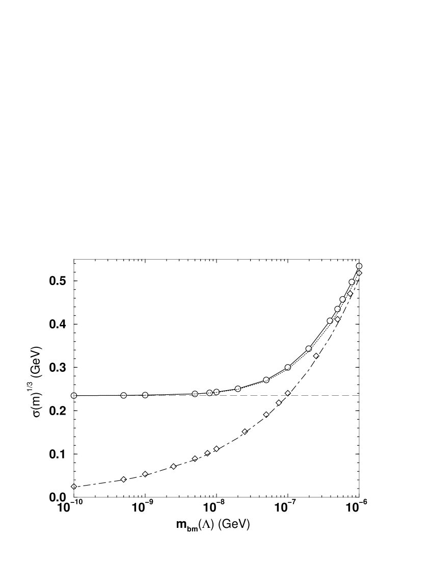
Figure 1: Circles/solid-line: $\sigma(m)^{1/3}$ in Eq. (37) as a function of the current-quark bare-mass, evaluated using the dressed-quark propagator obtained in the model of Ref. mr97 ; dashed line: the model’s value of $(-\langle\bar{q}q\rangle^{0}_{\zeta=1\,{\rm GeV}})=(0.24\,{\rm GeV})^{3}$; and dotted line: Eq. (40). Diamonds: $\sigma(m)^{1/3}$ evaluated in a non-confining version of the model; dot-dashed line: Eq. (40) with $\langle\bar{q}q\rangle^{0}\equiv 0$.

The discussion establishes that $\sigma(m,\zeta)$ has a regular chiral limit in QCD and is a monotonically increasing convex-up function. It follows that $\sigma(m,\zeta)$ has a spectral representation:

$$\sigma(m,\zeta)=2m\int_{0}^{\Lambda}\frac{\rho(\lambda)}{\lambda^{2}+m^{2}}\,.$$ (41)

This lays the vital plank in a veracious connection between the condensates in Eqs. (1) and (8). On the domain specified by Eq. (39), the behaviour of $\sigma(m,\zeta)$ in Eq. (37) is given by Eq. (40), which yields, via Eq. (33),

$$\pi\,\rho(\lambda)=-\langle\bar{q}q\rangle^{0}_{\zeta}+Z_{4}(\zeta,\Lambda)\,\frac{N_{c}}{4\pi}\,\lambda^{3}+\ldots$$ (42)

where the ellipsis denotes contributions from the higher-order terms implicit in Eq. (40).

III.2 Comparison with a lattice-QCD simulation

In Fig. 2 we plot the spectral density of the staggered Dirac operator in quenched $SU(3)$ gauge theory calculated with $3000$ configurations obtained on a $V=4^{4}$-lattice, in the vicinity of the deconfining phase transition at $\beta\gtrsim 5.6$. Details of the simulation are given in Ref. Harald . Dimensioned quantities are measured in units of $1/a$, where $a$ is the lattice spacing, and it is $\rho(\lambda)/V$ that should be compared with the continuum spectral density.

While the effect of finite lattice volume is apparent in Fig. 2 for $\lambda a\gtrsim 0.1$, the behaviour at small $\lambda a$ is qualitatively in agreement with Eq. (42) and Fig. 1: a nonzero OPE condensate dominates the Dirac spectrum in the confined domain; and it vanishes in the deconfined domain whereupon $\rho(0)=0$ and the perturbative evolution, Eq. (35), is manifest.

To be more quantitative, we note that at $\beta=5.4$, $\rho(0)a^{3}\approx 70$, so that

$$\pi\rho(0)a^{3}/V\approx(0.95)^{3}.$$ (43)

The value of the lattice spacing was not measured in Ref. Harald but one can nevertheless assess the scale of Eq. (43) by supposing $a\sim 0.3\,{\rm fm}\sim 0.3/\Lambda_{\rm QCD}$, a value typical of small couplings, $\beta$, wherewith the r.h.s. is $\sim(3\Lambda_{\rm QCD})^{3}\!$. This is too large but not unreasonable given the parameters of the simulation, its errors and the systematic uncertainties in our estimate. One can also fit the lattice data at $\beta=5.8$, whereby one finds $\rho(\lambda)\propto\lambda^{3}$ on $\lambda<0.1$ but with a proportionality constant larger than that anticipated from perturbation theory; viz. Eq. (42). Some mismatch is to be expected because at $\beta=5.8$ one has only just entered the deconfined domain and close to the transition boundary nonperturbative effects are still material, as seen, e.g., in the heavy-quark potential and equation of state edwinechaya . It is a modern challenge to determine those gauge couplings and lattice parameters for which the data are quantitatively consistent with Eq. (42).

Figure 2: Spectral density of the staggered Dirac operator in quenched $SU(3)$ gauge theory calculated on a $4^{4}$-lattice. (Measured in units of the lattice spacing.) The deconfinement transition takes place at $\beta\gtrsim 5.6$.

IV Epilogue

We verified that the gauge-invariant trace of the massive dressed-quark propagator possesses a spectral representation when considered as a function of the current-quark mass. This is key to establishing that the OPE condensate, which sets the ultraviolet scale for the momentum-dependence of the trace of the dressed-quark propagator, does indeed measure the density of far-infrared eigenvalues of the gauge-averaged massless Dirac operator, à la the Banks-Casher relation. This relation is intuitively appealing because a measurable accumulation of eigenvalues of the massless Dirac operator at zero-virtuality expresses a mass gap in its spectrum.

In practice, there are three main parameters in a simulation of lattice-QCD: the lattice volume, characterised by a length $L$; the lattice spacing, $a$; and the current-quark mass, $m$. So long as the lattice size is large compared with the current-quark’s Compton wavelength; viz., $L\gg 1/m$, then dynamical chiral symmetry breaking can be expressed in the simulation. Supposing that to be the case then, as we have explicated, so long as the lattice spacing is small compared with the current-quark’s Compton wavelength; i.e., $a\ll 1/m\ll L$,

$$\pi\,\rho(0)\approx-\langle\bar{q}q\rangle^{0}_{1/a}\,,$$ (44)

where the r.h.s. is the scale-dependent OPE condensate [$\zeta=\Lambda=1/a$ in Eq. (42)].

In our continuum analysis we found that one requires $am\lesssim(a\Lambda_{\rm QCD})^{3}$ if $\rho(\lambda=0)$ is to provide a veracious estimate of the OPE condensate. The residue at the lowest-mass pole in the flavour-nonsinglet pseudoscalar vacuum polarisation provides a measure of the OPE condensate that is accurate for larger current-quark masses.

Appendix A Model Gap Equation

The gap equation’s kernel is built from a product of the dressed-gluon propagator and dressed-quark-gluon vertex. It can be calculated in perturbation theory but that is inadequate for the study of intrinsically nonperturbative phenomena. To make model-independent statements about DCSB one must employ an alternative systematic and chiral symmetry preserving truncation scheme.

The leading order term in one such scheme truncscheme is the renormalisation-group-improved rainbow truncation of the gap equation $(Q=p-q)$:

$$S(p)^{-1}=Z_{2}\,(i\gamma\cdot p+m^{\rm bm})$$ (45)

$$+ \int^{\Lambda}_{q}\,{\cal G}(Q^{2})D_{\mu\nu}^{\rm free}(Q)\frac{\lambda^{a}}{2}\gamma_{\mu}S(q)\frac{\lambda^{a}}{2}\gamma_{\nu}\,.$$

The ultraviolet ($Q^{2}\gtrsim 1\,$GeV${}^{2})$ behaviour of ${\cal G}(Q^{2})$ in Eq. (45) is fixed by the known behaviour of the quark-antiquark scattering kernel mr97 . The form of that kernel on the infrared domain is currently unknown and a model is employed to complete the specification of the kernel. An efficacious form is mr97

$$\frac{{\cal G}(Q^{2})}{Q^{2}}=8\pi^{4}D\delta^{4}(k)+\frac{4\pi^{2}}{\omega^{6}}DQ^{2}{\rm e}^{-Q^{2}/\omega^{2}}$$ (46)

$$+4\pi\,\frac{\gamma_{m}\pi}{\frac{1}{2}\ln\left[\tau+\left(1+Q^{2}/\Lambda_{\rm QCD}^{2}\right)^{2}\right]}{\cal F}(Q^{2})\,,$$

where: ${\cal F}(Q^{2})=[1-\exp(-Q^{2}/[4m_{t}^{2}])]/Q^{2}$, $m_{t}$ $=$ $0.5\,$GeV; $\tau={\rm e}^{2}-1$; $\gamma_{m}=12/(33-2N_{f})$, $N_{f}=4$; and $\Lambda_{\rm QCD}=\Lambda^{(4)}_{\overline{\rm MS}}=0.234\,$GeV. The true parameters in Eq. (46) are $D$ and $\omega$, however, they are not independent: in fitting, a change in one is compensated by altering the other, with fitted observables changing little along a trajectory $\omega\,D=(0.6\,{\rm GeV})^{3}$. Herein we used

$$D=(0.884\,{\rm GeV})^{2}\,,\;\omega=0.3\,{\rm GeV}.$$ (47)

A non-confining model is obtained with $D=0$.

Equation (45), is readily solved for the dressed-quark propagator, with the renormalisation constants fixed via Eq. (11). That solution provides the elements used in the illustration of Sec. III.

References

- (1) K.D. Lane, Phys. Rev. D 10, 2605 (1974); H.D. Politzer, Nucl. Phys. B 117, 397 (1976).
- (2) P. Maris and C.D. Roberts, Phys. Rev. C 56, 3369 (1997).
- (3) C.D. Roberts and A.G. Williams, Prog. Part. Nucl. Phys. 33, 477(1994).
- (4) P.O. Bowman, U.M. Heller and A.G. Williams, Phys. Rev. D 66, 014505 (2002).
- (5) J.B. Zhang, F.D.R. Bonnet, P.O. Bowman, D.B. Leinweber and A.G. Williams, “Towards the Continuum Limit of the Overlap Quark Propagator in Landau Gauge,” hep-lat/0208037.
- (6) P. Maris, A. Raya, C.D. Roberts and S.M. Schmidt, “Confinement and dynamical chiral symmetry breaking,” to appear in the proceedings of Quark Nuclear Physics 2002, nucl-th/0208071.
- (7) In our Euclidean metric: ; ; and .
- (8) In deriving Eq. (4), zero modes have been neglected, which is justified under broad conditions leutwyler .
- (9) H. Leutwyler and A. Smilga, Phys. Rev. D 46, 5607 (1992).
- (10) T. Banks and A. Casher, Nucl. Phys. B 169, 103 (1980).
- (11) E. Marinari, G. Parisi and C. Rebbi, Phys. Rev. Lett. 47, 1795 (1981).
- (12) E. Bittner, H. Markum and R. Pullirsch, Nucl. Phys. Proc. Suppl. 96, 189 (2001).
- (13) E. Bittner, M.P. Lombardo, H. Markum and R. Pullirsch, Nucl. Phys. Proc. Suppl. 94, 445 (2001).
- (14) T. Bielefeld, S. Hands, J.D. Stack and R.J. Wensley, Phys. Lett. B 416, 150 (1998).
- (15) J.J. Verbaarschot, Phys. Rev. Lett. 72, 2531 (1994); J.J. Verbaarschot and T. Wettig, Ann. Rev. Nucl. Part. Sci. 50, 343 (2000).
- (16) M.E. Berbenni-Bitsch, S. Meyer, A. Schäfer, J.J. Verbaarschot and T. Wettig, Phys. Rev. Lett. 80, 1146 (1998); M. Göckeler, H. Hehl, P.E. Rakow, A. Schäfer and T. Wettig, Phys. Rev. D 59, 094503 (1999); R.G. Edwards, U.M. Heller, J.E. Kiskis and R. Narayanan, Phys. Rev. Lett. 82, 4188 (1999); B.A. Berg, H. Markum, R. Pullirsch and T. Wettig, Phys. Rev. D 63, 014504 (2001); P.H. Damgaard, U.M. Heller, R. Niclasen and K. Rummukainen, Phys. Lett. B 495, 263 (2000); B.A. Berg, U.M. Heller, H. Markum, R. Pullirsch and W. Sakuler, Phys. Lett. B 514, 97 (2001).
- (17) P. Maris, C.D. Roberts and P.C. Tandy, Phys. Lett. B 420, 267 (1998).
- (18) C.D. Roberts and S.M. Schmidt, Prog. Part. Nucl. Phys. 45, S1 (2000); R. Alkofer and L.v. Smekal, Phys. Rept. 353, 281 (2001).
- (19) M.A. Ivanov, Yu.L. Kalinovsky and C.D. Roberts, Phys. Rev. D 60, 034018 (1999).
- (20) C.D. Roberts, Nucl. Phys. Proc. Suppl. 108, 227 (2002)
- (21) P. Hernandez, K. Jansen, L. Lellouch and H. Wittig, JHEP 0107, 018 (2001); A. Duncan, S. Pernice and J. Yoo, Phys. Rev. D 65, 094509 (2002).
- (22) P. Maris and P.C. Tandy, Phys. Rev. C 60, 055214 (1999).
- (23) K. Zyablyuk, JHEP 0006, 025 (2000).
- (24) F.T. Hawes, C.D. Roberts and A.G. Williams, Phys. Rev. D 49, 4683 (1994); A. Bender, D. Blaschke, Yu.L. Kalinovsky and C.D. Roberts, Phys. Rev. Lett. 77, 3724 (1996); F.T. Hawes, P. Maris and C.D. Roberts, Phys. Lett. B 440, 353 (1998).
- (25) E. Laermann, Fiz. Élem. Chastits At. Yadra 30 (1999) 720 (Phys. Part. Nucl. 30 (1999) 304).
- (26) A. Bender, C.D. Roberts and L. v. Smekal, Phys. Lett. B 380, 7 (1996); A. Bender, W. Detmold, A.W. Thomas and C.D. Roberts, Phys. Rev. C 65, 065203 (2002).