AN OVERVIEW OF THE HYPERCENTRAL CONSTITUENT QUARK MODEL

Abstract

We report on the recent results of the hypercentral Constituent Quark Model (hCQM). The model contains a spin independent three-quark interaction which is inspired by Lattice QCD calculations and reproduces the average energy values of the $SU(6)$ multiplets. The splittings are obtained with a $SU(6)$-breaking interaction, which can include also an isospin dependent term. The model has been used for predictions concerning the electromagnetic transition form factors giving a good description of the medium $Q^{2}$-behaviour. In particular the calculated helicity amplitude $A_{\frac{1}{2}}$ for the $S_{11}(1535)$ resonance agrees very well with the recent CLAS data. Furthermore, we have shown for the first time that the decreasing of the ratio of the elastic form factors of the proton is due to relativistic effects. Finally, the elastic nucleon form factors have been calculated using a relativistic version of the hCQM and a relativistic quark current.

1 Introduction

In recent years much attention has been devoted to the description of the internal nucleon structure in terms of quark degrees of freedom. Besides the now classical Isgur-Karl model [1], the Constituent Quark Model has been proposed in quite different approaches: the algebraic one [2], the hypercentral formulation [3] and the chiral model [4, 5]. In the following the hypercentral Constituent Quark Model (hCQM), which has been used for a systematic calculation of various baryon properties, will be briefly reviewed.

2 The hypercentral model

The experimental $4-$ and $3-$star non strange resonances can be arranged in $SU(6)-$multiplets (see Fig. 1). This means that the quark dynamics has a dominant $SU(6)-$invariant part, which accounts for the average multiplet energies. In the hCQM it is assumed to be [3]

$$V(x)=-\frac{\tau}{x}~{}+~{}\alpha x,$$ (1)

where $x$ is the hyperradius

$$x=\sqrt{{\vec{\rho}}^{2}+{\vec{\lambda}}^{2}}~{}~{},$$ (2)

where $\vec{\rho}$ and $\vec{\lambda}$ are the Jacobi coordinates describing the internal quark motion. The dependence of the potential on the hyperrangle $\xi=arctg(\frac{{\rho}}{{\lambda}})$ has been neglected.

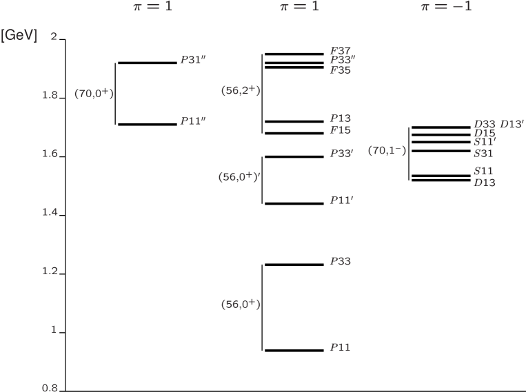
Figure 1: The experimental spectrum of the 4- and 3-star non strange resonances. On the left the standard assignements to $SU(6)$ multiplets is reported, with the total orbital angular momentum and the parity.

Interactions of the type linear plus Coulomb-like have been used since time for the meson sector, e.g. the Cornell potential. This form has been supported by recent Lattice QCD calculations [6]. In the case of baryons a so called hypercentral approximation has been introduced [7, 8], which amounts to average any two-body potential for the three quark system over the hyperangle $\xi$ and works quite well, specially for the lower part of the spectrum [9]. In this respect, the hypercentral potential Eq.1 can be considered as the hypercentral approximation of the Lattice QCD potential. On the other hand, the hyperradius $x$ is a collective coordinate and therefore the hypercentral potential contains also three-body effects.

The hypercoulomb term $1/x$ has important features [3, 10]: it can be solved analytically and the resulting form factors have a power-law behaviour, at variance with the widely used harmonic oscillator; moreover, the negative parity states are exactly degenerate with the first positive parity excitation, providing a good starting point for the description of the spectrum.

The splittings within the multiplets are produced by a perturbative term breaking $SU(6)$, which as a first approximation can be assumed to be the standard hyperfine interaction $H_{hyp}$ [1]. The three quark hamiltonian for the hCQM is then:

$$H=\frac{p_{\lambda}^{2}}{2m}+\frac{p_{\rho}^{2}}{2m}-\frac{\tau}{x}~{}+~{}\alpha x+H_{hyp},$$ (3)

where $m$ is the quark mass (taken equal to $1/3$ of the nucleon mass). The strength of the hyperfine interaction is determined in order to reproduce the $\Delta-N$ mass difference, the remaining two free parameters are fitted to the spectrum, reported in Fig. 2, leading to the following values:

$$\alpha=1.16~{}fm^{-2},~{}~{}~{}~{}\tau=4.59~{}.$$ (4)

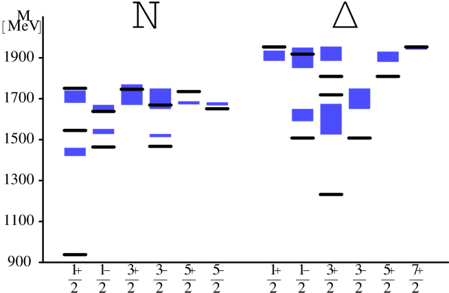
Figure 2: The spectrum obtained with the hypercentral model Eq. (3) and the parameters Eq. (4) (full lines)), compared with the experimental data of PDG [11] (grey boxes).

Keeping these parameters fixed, the model has been applied to calculate various physical quantities of interest: the photocouplings [12], the electromagnetic transition amplitudes [13], the elastic nucleon form factors [14] and the ratio between the electric and magnetic proton form factors [15]. Some results of such parameter free calculations are presented in the next section.

3 The results

The electromagnetic transition amplitudes, $A_{1/2}$ and $A_{3/2}$, are defined as the matrix elements of the transverse electromagnetic interaction, $H_{e.m.}^{t}$, between the nucleon, $N$, and the resonance, $B$, states:

$$\begin{array}[]{rcl}A_{1/2}&=&\langle B,J^{\prime},J^{\prime}_{z}=\frac{1}{2}\ |H_{em}^{t}|N,J~{}=~{}\frac{1}{2},J_{z}=-\frac{1}{2}\ \rangle\\ &&\\ A_{3/2}&=&\langle B,J^{\prime},J^{\prime}_{z}=\frac{3}{2}\ |H_{em}^{t}|N,J~{}=~{}\frac{1}{2},J_{z}=\frac{1}{2}\ \rangle\\ \end{array}$$ (5)

The transition operator is assumed to be

$$H^{t}_{em}~{}=~{}-~{}\sum_{j=1}^{3}~{}\left[\frac{e_{j}}{2m_{j}}~{}(\vec{p_{j}}\cdot\vec{A_{j}}~{}+~{}\vec{A_{j}}\cdot\vec{p_{j}})~{}+~{}2\mu_{j}~{}\vec{s_{j}}\cdot(\vec{\nabla}\times\vec{A_{j}})\right]~{}~{},$$ (6)

where spin-orbit and higher order corrections are neglected [16, 17]. In Eq. (6) $~{}~{}m_{j}$, $e_{j}$, $\vec{s_{j}}$ , $\vec{p_{j}}$ and $\mu_{j}~{}=~{}\frac{ge_{j}}{2m_{j}}$ denote the mass, the electric charge, the spin, the momentum and the magnetic moment of the j-th quark, respectively, and $\vec{A_{j}}~{}=~{}\vec{A_{j}}(\vec{r_{j}})$ is the photon field; quarks are assumed to be pointlike.

The proton photocouplings of the hCQM [12] (Eq. (5) calculated at the photon point), in comparison with other calculations [2, 17, 21], have the same overall behaviour, having the same SU(6) structure in common, but in many cases they all show a lack of strength.

Figure 3: The helicity amplitudes for the $D_{13}(1520)$ resonance, calculated with the hCQM of Eqs. (3) and (4) and the electromagnetic transition operator of Eq. (6) (full curve, [13]). The dashed curve is obtained with the analytical version of the hCQM ([10]), where the behaviour of the quark wave function is determined mainly by the hypercoulomb potential. The data are from the compilation of ref. [19]

Figure 4: The helicity amplitude for the $S_{11}(1535)$ resonance, calculated with the hCQM of Eqs. (3) and (4) and the electromagnetic transition operator of Eq. (6) (dashed curve, [13]) and the model of ref.[21]. The data are taken from the compilation of ref. [22]

Taking into account the $Q^{2}-$behaviour of the transition matrix elements of Eq. (5), one can calculate the hCQM helicity amplitudes in the Breit frame [13]. The hCQM results for the $D_{13}(1520)$ and the $S_{11}(1535)$ resonances [13] are given in Fig. 3 and 4, respectively. The agreement in the case of the $S_{11}$ is remarkable, the more so since the hCQM curve has been published three years in advance with respect to the recent TJNAF data [20].

In general the $Q^{2}$-behaviour is reproduced, except for discrepancies at small $Q^{2}$, especially in the $A^{p}_{3/2}$ amplitude of the transition to the $D_{13}(1520)$ state. These discrepancies, as the ones observed in the photocouplings, can be ascribed either to the non-relativistic character of the model or to the lack of explicit quark-antiquark configurations, which may be important at low $Q^{2}$ . The kinematical relativistic corrections at the level of boosting the nucleon and the resonance states to a common frame are not responsible for these discrepancies, as we have demonstrated in Ref. [23]. Similar results are obtained for the other negative parity resonances [13]. It should be mentioned that the r.m.s. radius of the proton corresponding to the parameters of Eq. (4) is $0.48~{}fm$, which is just the value obtained in [16] in order to reproduce the $D_{13}$ photocoupling. Therefore the missing strength at low $Q^{2}$ can be ascribed to the lack of quark-antiquark effects, probably more important in the outer region of the nucleon.

4 The isospin dependence

The well known Guersey-Radicati mass formula [24] contains a flavour dependent term, which is essential for the description of the strange baryon spectrum. In the chiral Constituent Quark Model [4, 5], the non confining part of the potential is provided by the interaction with the Goldstone bosons, giving rise to a spin- and flavour-dependent part, which is crucial in this approach for the description of the lower part of the spectrum. More generally, one can expect that the quark-antiquark pair production can lead to an effective residual quark interaction containing an isospin (flavour) dependent term.

Figure 5: The spectrum obtained with the hypercentral model containing isospin dependent terms Eq. (7) [25] (full lines)), compared with the experimental data of PDG [11] (grey boxes).

Therefore, we have introduced isospin dependent terms in the hCQM hamiltonian. The complete interaction used is given by [25]

$$H_{int}~{}=~{}V(x)+H_{\mathrm{S}}+H_{\mathrm{I}}+H_{\mathrm{SI}}~{},$$ (7)

where $V(x)$ is the linear plus hypercoulomb SU(6)-invariant potential of Eq. 1, while the remaining terms are the residual SU(6)-breaking interaction, responsible for the splittings within the multiplets. ${H}_{\mathrm{S}}$ is a smeared standard hyperfine term, ${H}_{\mathrm{I}}$ is isospin dependent and ${H}_{\mathrm{SI}}$ spin-isospin dependent. The resulting spectrum for the 3*- and 4*- resonances is shown in Fig. 5 [25]. The contribution of the hyperfine interaction to the $N-\Delta$ mass difference is only about $35\%$, while the remaining splitting comes from the spin-isospin term, $(50\%)$, and from the isospin one, $(15\%)$. It should be noted that the position of the Roper and the negative parity states is well reproduced.

5 Relativity

The relativistic effects that one can introduce starting from a non relativistic quark model are: a) the relativistic kinetic energy; b) the boosts from the rest frames of the initial and final baryon to a common (say the Breit) frame; c) a relativistic quark current. All these features are not equivalent to a fully relativistic dynamics, which is still beyond the present capabilities of the various models.

The potential of Eq.1 has been refitted using the correct relativistic kinetic energy

$$H_{rel}=\sum_{i<j}\sqrt{p_{ij}^{2}+m^{2}}-\frac{\tau}{x}~{}+~{}\alpha x+H_{hyp}.$$ (8)

The resulting spectrum is not much different from the non relativistic one and the parameters of the potential are only slightly modified.

Figure 6: The electric proton form factor, calculated with the relativistic hCQM of Eq. (8) and a relativistic quark current [27].

Figure 7: The magnetic proton form factor, calculated with the relativistic hCQM of Eq. (8) and a relativistic quark current [27].

Figure 8: The ratio between the electric and magnetic proton form factors, calculated with the relativistic hCQM of eq. (8) and a relativistic current [27], compared with the TJNAF data [26, 28].

The boosts and a relativistic quark current expanded up to lowest order in the quark momenta has been used both for the elastic form factors of the nucleon [14] and the helicity amplitudes [23]. In the latter case, as already mentioned, the relativistic effects are quite small and do not alter the agreement with data discussed previously. For the elastic form factors, the relativistic effects are quite strong and bring the theoretical curves much closer to the data; in any case they are responsible for the decrease of the ratio between the electric and magnetic proton form factors, as it has been shown for the first time in Ref.  [15], in qualitative agreement with the recent Jlab data [26].

A relativistic quark current, with no expansion in the quark momenta, and the boosts to the Breit frame have been applied to the calculation of the elastic form factors in the relativistic version of the hCQM Eq. (8) [27]. The resulting theoretical form factors of the proton, calculated, it should be stressed, without free parameters and assuming pointlike quarks, are good (see Figs.  6 and 7), with some discrepancies at low $Q^{2}$, which, as discussed previously, can be attributed to the lacking of the quark-antiquark pair effects. The corresponding ratio between the electric and magnetic proton form factors is given in Fig. 8: the deviation from unity reaches almost the $50\%$ level, not far from the new TJNAF data [28].

6 Conclusions

The hCQM is a generalization to the baryon sector of the widely used quark-antiquark potential containing a coulomb plus a linear confining term. The three free parameters have been adjusted to fit the spectrum [3] and then the model has been used for a systematic calculation of various physical quantities: the photocouplings [12], the helicity amplitudes for the electromagnetic excitation of negative parity baryon resonances [13, 23], the elastic form factors of the nucleon [14, 27] and the ratio between the electric and magnetic proton form factors [15, 27]. The agreement with data is quite good, specially for the helicity amplitudes, which are reproduced in the medium-high $Q^{2}$ behaviour, leaving some discrepancies at low (or zero) $Q^{2}$, where the lacking quark-antiquark contributions are expected to be effective. It should be noted that the hypercoulomb term in the potential is the main responsible of such an agreement [10], while for the spectrum a further fundamental aspect is provided by the isospin dependent interactions [25].

References

- [1] N. Isgur and G. Karl, Phys. Rev. D18, 4187 (1978); D19, 2653 (1979); D20, 1191 (1979); S. Godfrey and N. Isgur, Phys. Rev. D32, 189 (1985); S. Capstick and N. Isgur, Phys. Rev. D 34,2809 (1986)
- [2] R. Bijker, F. Iachello and A. Leviatan, Ann. Phys. (N.Y.) 236, 69 ( 1994)
- [3] M. Ferraris, M.M. Giannini, M. Pizzo, E. Santopinto and L. Tiator, Phys. Lett. B364, 231 (1995).
- [4] L. Ya. Glozman and D.O. Riska, Phys. Rep. C268, 263 (1996).
- [5] L. Ya. Glozman, Z. Papp, W. Plessas, K. Varga and R. F. Wagenbrunn, Phys. Rev. C57, 3406 (1998); L. Ya. Glozman, W. Plessas, K. Varga and R. F. Wagenbrunn, Phys. Rev. D58, 094030 (1998).
- [6] G. Bali et al., Phys. Rev. D51, 5165 (1995).
- [7] P. Hasenfratz, R.R. Horgan, J. Kuti and J.M. Richard, Phys. Lett. B94, 401 (1980)
- [8] J.-M. Richard, Phys. Rep. C 212, 1 (1992)
- [9] M. Fabre de la Ripelle and J. Navarro, Ann. Phys. (N.Y.) 123, 185 (1979).
- [10] E. Santopinto, F. Iachello and M.M. Giannini, Nucl. Phys. A623, 100c (1997); Eur. Phys. J. A1, 307 (1998)
- [11] Particle Data Group, Eur. Phys. J. C15, 1 (2000).
- [12] M. Aiello, M. Ferraris, M.M. Giannini, M. Pizzo and E. Santopinto, Phys. Lett. B387, 215 (1996).
- [13] M. Aiello, M. M. Giannini and E. Santopinto, J. Phys. G: Nucl. Part. Phys. 24, 753 (1998)
- [14] M. De Sanctis, E. Santopinto and M.M. Giannini, Eur. Phys. J. A1, 187 (1998).
- [15] M. De Sanctis, M.M. Giannini, L. Repetto and E. Santopinto, Phys. Rev. C62, 025208 (2000).
- [16] L. A. Copley, G. Karl and E. Obryk, Phys. Lett. 29, 117 (1969).
- [17] R. Koniuk and N. Isgur, Phys. Rev. D21, 1868 (1980).
- [18] F. E. Close and Z. Li, Phys. Rev. D42, 2194 (1990); Z. Li and F.E. Close, Phys. Rev. bf D42, 2207 (1990).
- [19] V. D. Burkert, private communication
- [20] R.A. Thompson et al., Phys. Rev. Lett. 86, 1702 (2001).
- [21] S. Capstick and B.D. Keister, Phys. Rev.D 51, 3598 (1995)
- [22] V. D. Burkert,arXiv:hep-ph/0207149.
- [23] M. De Sanctis, E. Santopinto and M.M. Giannini, Eur. Phys. J. A2, 403 (1998).
- [24] F. Guersey and L.A. Radicati, Phys. Rev. Lett. 13, 173 (1964); M. Gell-Mann, Phys. Rev. 125, 1067 (1962); S. Okubo, Prog. Theor. Phys. 27, 949 (1962)
- [25] M.M. Giannini, E. Santopinto and A, Vassallo, Eur. Phys. J. A12, 447 (2001).
- [26] M.K. Jones et al., Phys. Rev. Lett. B84,1398 (2000).
- [27] M. De Sanctis, M.M. Giannini, E. Santopinto and A. Vassallo, to be published.
- [28] O. Gayon et al., Phys. Rev. Lett. 88, 092301 (2002).