Tests of the random phase approximation for transition strengths

Abstract

We investigate the reliability of transition strengths computed in the random-phase approximation (RPA), comparing with exact results from diagonalization in full $0\hbar\omega$ shell-model spaces. The RPA and shell-model results are in reasonable agreement for most transitions; however some very low-lying collective transitions, such as isoscalar quadrupole, are in serious disagreement. We suggest the failure lies with incomplete restoration of broken symmetries in the RPA. Furthermore we prove, analytically and numerically, that standard statements regarding the energy-weighted sum rule in the RPA do not hold if an exact symmetry is broken.

I Introduction

Electromagnetic and weak transitions provide important probes of nuclear wavefunctions. Exact numerical solutions of the many-body Schrödinger equation are very difficult, so theorists have devised a number of approximations. Transitions offer a serious test of the model wavefunctions, not only in comparison to experiment but also between approximations.

One of the most successful approximations is the interacting shell model (SM), which diagonalizes an effective Hamiltonian in a restricted space, providing good description of the observed low lying states for a wide range of mass numbers. The SM wavefunctions successfully describe electromagnetic and weak transitions, in good agreement (albeit sometimes requiring effective couplings) with the experimental data; for this reason, in this paper we consider SM results to be exact. Due to the computational burden which increases with mass number, however, full $0\hbar\omega$ SM calculations are presently limited to light and medium nuclei ($A<80$).

Another approximation, which works surprisingly well considering its simplicity, is mean-field theory, e.g., Hartree-Fock (HF) theory. In this approach, the particles are uncorrelated and move in an average potential which replaces the two-body interaction; the ground state is determined by energy minimization. Starting from the HF solution, the Tamm-Dancoff approximation (TDA) constructs excited states by assuming them to be mixtures of one particle, one hole (1p-1h) configurations. The HF+TDA is the simplest model for ground and excited state wavefunctions. There are also limitations of this model: the ground state wavefunction is a single Slater determinant which can break symmetries of the Hamiltonian and neglects particle-hole correlations arising from the residual interaction ring .

The random phase approximation (RPA) is a generalization of the TDA, which takes into account the residual interaction by adding 2p-2h correlations in the ground state. (An important extension is the quasiparticle RPA or QRPA; because it accounts for nonperturbative pairing effects, it is often considered a superior approach. In this paper we restrict ourselves to number-conserving RPA.) The excited states, as in the TDA, remain 1p-1h mixtures. Is this the case? That is, are the excited states mainly mixtures of 1p-1h correlations? The answer is no: one knows from SM calculations that, for example, the first excited state in ¹⁶O has a predominant 4p-4h character haxton1990 , outside the RPA model space. Is therefore no surprise that RPA fails in these situations.

Despite known limitations, the RPA (or QRPA) has been widely applied for decades to evaluate spectra and transition strengths in nuclei. The reason, aside from computational simplicity, is that it is frequently, although not always kuo1970 ; m2strength , in close agreement with experiment. Thus, RPA was the method of choice for description of negative parity states in closed shell nuclei kuo1970 ; ullah69 ; blomqvist1969 ; true1971 and in open shell nuclei rowe1970 . RPA and QRPA calculations (sometimes including continuum states) using phenomenological interactions have been successful in describing the experimental position of giant resonances Goeke82 , particularly E1 rowe1970 ; e1 and M1 soloviev1999 from electron or proton scattering, or Gamow-Teller resonances grimes1996 . In general, however, the description of low-lying transitions is poor grimes1996 ; lowstates . Other studies have used QRPA to compute transitions of interest for astrophysics but did not directly compare to experiment jameel ; hamamoto .

What about tests of RPA against exact models? Until recently there was no thorough test of the HF+RPA against an exact non-trivial model for binding energies. We performed such a test for a large number of nuclei and found that in general HF+RPA is a good approximation to the exact shell-model binding energy stetcu2002 , although with some significant failures. Tests of transitions have been also mainly against ‘toy’ models lipkinTest1 ; lipkinTest2 ; engel1997 , although the QRPA has been tested against exact diagonalization in the full SM space for $\beta^{\pm}$ or double $\beta$ decays lauritzen ; civitarese ; Zhao1993 ; auerbach , with mixed success. Broader tests of RPA transitions strengths against an exact model, e.g., SM, has not been done. To address this issue, this paper tests the RPA against full $0\hbar\omega$ calculation for several nuclei in the sd and pf shells for electromagnetic transitions. Unlike previous tests however, we consider mean-field solutions which break the rotational symmetry.

We find that, in general, the RPA produces a reasonable approximation to the exact (SM) transitions. The most significant failures are for certain low-lying collective states. We understand these failures through the incomplete restoration of broken symmetries and the nature of collective giant resonances.

The Brown-Bosterli schematic model ring ; brown1959 provides insight into giant collective resonances. It assumes the model Hamiltonian to be single-particle energies plus a separable residual interaction. In both the TDA and the RPA, all of the Brown-Bosterli transition strength is to a single state, the collective state, which is a model for giant resonances. If the residual interaction is repulsive, then the collective state will be at high energy. If the interaction is attractive, then the collective state will be low in energy. In more realistic models, of course, the residual interaction includes more complicated two-body forces, causing the giant resonance to spread over many states. The important lesson of the Brown-Bosterli model, however, is that an attractive interaction, such as isoscalar quadrupole-quadrupole, leads to large collective transitions low in the spectrum, while repulsive interactions, such as $\sigma\cdot\sigma$, produce collective transitions lying higher in the spectrum.

Breaking of symmetries can result in low-lying collectivity being subsumed into the ground state. For example, the strongly attractive isoscalar quadrupole-quadrupole interaction leads to a quadrupole deformation in the HF state. While the RPA identifies broken symmetries, restoration of symmetry is incomplete. This point is not fully explicated or understood in the literature, but our calculations here provide further evidence, as discussed in detail in Sec. III.2.

The paper is organized as follows. Sec. II presents briefly the interacting SM and the RPA formalisms, with emphasis on their application to transition strengths. In Sec. III we compare the SM and RPA transition strengths and distribution properties for several nuclides, while in Sec. IV we summarize results. In the Appendix we consider in some detail the effect of breaking of exact symmetries on transition strength sum rules.

II formalism

II.1 General Overview

In this section we briefly present the treatment of transitions in both SM and RPA. Before giving any specific details, we review some general concepts.

A primary goal is, given the Hamiltonian $H$, to calculate solutions to the eigenvalue equation

$$H|\nu\rangle=E_{\nu}|\nu\rangle.$$ (1)

Suppose we have solved Eq. (1), either in the SM or RPA. The transition strength from an excited to the ground-state is given by the square of the matrix element,

$$S(0\rightarrow\nu)=|\langle\nu|F|0\rangle|^{2},$$

while the quantity

$$S_{k}=\sum_{\nu}(E_{\nu}-E_{0})^{k}|\langle\nu|F|0\rangle|^{2}$$ (2)

is the (energy weighted) sum rule of order $k$. In this equation, $\nu$ runs over all states, $0$ stands for the ground state, and $F$ is an arbitrary transition operator. Particularly important is $S_{0}$, which is the total transition strength from the ground state to excited states, and which can be rewritten as a ground state expectation value:

$$S_{0}\equiv\sum_{\nu}|\langle\nu|F|0\rangle|^{2}=\langle 0|F^{\dagger}F|0\rangle.$$ (3)

(In most realistic applications the transition operator is a spherical tensor of rank $K$, $F_{KM}$, which has the property $F_{KM}^{\dagger}=(-1)^{M}F_{K-M}$ edmonds . Then properly the total strength in Eq. (3) should be

$$S_{0}=\sum_{M}(-1)^{M}\langle 0|F_{K-M}F_{KM}|0\rangle,$$ (4)

and similarly for the double commutator in the energy-weighted sum rule, etc. To avoid clutter we drop the sum over $M$ and it should be assumed to be implicit. )

In fact one can write all the sum rules of order $k$ as expectation values, most famously the linear energy-weighted sum rule:

$$S_{1}=\sum_{\nu}(E_{\nu}-E_{0})|\langle 0|F|\nu\rangle|^{2}=\frac{1}{2}\langle 0|[F,[H,F]]|0\rangle.$$ (5)

We will often characterize our results in terms of the centroid, $\bar{S}$, and the width, $\Delta S$, of the transition strengths, defined in terms of $S_{1}$ and $S_{2}$

$$\bar{S}=\frac{S_{1}}{S_{0}},\;\;\,\,\,\,\Delta S=\sqrt{\frac{S_{2}}{S_{0}}-\bar{S}^{2}}.$$ (6)

Both the centroid and the width characterize global properties of collective excitations.

II.2 Shell Model

In the interacting SM, the number of possible many-body configurations is restricted by two means: first, one assumes that only a limited number of nucleons interact (valence particles), the rest forming an inert core, and second, the active particles are restricted to a small number of single particle states (valence space). Usually, the valence space is restricted to a major oscillator shell. Diagonalization of an effective Hamiltonian provides the low lying states by means of the Lanczos algorithm Whitehead77 ; the corresponding wavefunctions are eigenstates of the parity, total angular momentum and isospin.

The reduction of the available single particle states and active particles makes the diagonalization numerically tractable. There is a downside though: in order to take into account the restriction of the Hilbert space one has to use modified (effective) operators to describe observables or transitions. In many cases a simple phenomenological use of either enhanced or quenched couplings, most famously the former for E2 transitions and the latter for Gamow-Teller transitions, yields good agreement with experiment.

In order to calculate transition strengths in SM, we have used the Lanczos moment method: the transition operator is applied on the initial state wavefunction. Then, the newly obtained state is used as the starting state, or pivot, for diagonalization by means of the Lanczos algorithm. The size of the pivot vector is the total transition strength $S_{0}$, and the overlap of the pivot with the final eigenstate, which it turns out can be read off trivially, is the transition amplitude. The interested reader is referred to Ref. LanczosMoment for details.

II.3 RPA

Several textbooks ring ; heyde cover the RPA, so we skip detailed derivation and just review principal steps.

The starting point of the RPA is a self-consistent mean-field solution, a Slater determinant which can break symmetries and which ignores correlations. This determines a deformed particle-hole basis, where the occupation numbers are zero for particle states and one for hole states.

The RPA ground state is defined as the vacuum for a set of quasiboson operators,

$$\beta_{\nu}|RPA\rangle=0,$$

while the excited states, approximate solutions of Eq. (1), are given by

$$|\nu\rangle=\beta_{\nu}^{\dagger}|RPA\rangle.$$

And because we assume the excited states to be 1p-1h correlations, one writes the quasiboson creation operators as ring

$$\beta_{\nu}^{\dagger}=\sum_{mi}\left(X_{mi}^{\nu}b_{mi}^{\dagger}-Y_{mi}^{\nu}b_{mi}\right),$$ (7)

where $b_{mi}^{\dagger}\approx c_{m}^{\dagger}c_{i}$ is the approximate boson mapping of the (deformed) fermion operators. We use the conventional notation that $m$, $n$ are unoccupied (particle) states, while $i$, $j$ are occupied (hole) states, respectively. Note that while in Eq. (7) the first terms describe particle-hole correlations on top of the HF state, the terms $Y^{\nu}_{mi}b_{mi}$ describe correlations coming from 2p-2h configurations in the ground state. In the RPA one assumes that the ground state is still very close to the HF solution, so that the hole-particle amplitudes $Y$ are much smaller than the particle-hole amplitudes $X$. Finally, the eigenvalue equation

$$\left(\begin{array}[]{cc}A&B\\ -B^{*}&-A^{*}\end{array}\right)\left(\begin{array}[]{c}X\\ Y\end{array}\right)=\Omega\left(\begin{array}[]{c}X\\ Y\end{array}\right),$$ (8)

determines the excitation energies $\Omega_{\nu}$ and the particle-hole $X$ and hole-particle amplitudes $Y$. $A$ and $B$ are matrices given by

$$A_{nj,mi}\equiv\left\langle HF\left|\left[\hat{c}^{\dagger}_{j}\hat{c}_{n},[\hat{H},\hat{c}^{\dagger}_{m}\hat{c}_{i}]\right]\right|HF\right\rangle,$$ (9)

$$B_{nj,mi}\equiv\left\langle HF\left|\left[[\hat{H},\hat{c}^{\dagger}_{n}\hat{c}_{j}],\hat{c}^{\dagger}_{m}\hat{c}_{i}\right]\right|HF\right\rangle.$$ (10)

Thouless showed thouless61 that if the HF solution corresponds to a minimum in energy surface, the corresponding RPA equation (8) has only real frequencies. In addition, if the Hartree-Fock state is invariant under some particle-hole transformation, such as rotation about an axis, this corresponds to a zero frequency RPA mode. Thus, the generators of symmetries broken by a mean-field solution are eigenvectors of Eq. (8) lying at at zero excitation energy. This is frequently interpreted as “approximate restoration of broken symmetries” ring ; in fact, it is more accurate to say that the RPA respects symmetries by separating out exactly spurious motion. In Sec. III we present evidence that significant part of the quadrupole response for even-even nuclei is still retained in the ground state, which suggests that broken symmetries are only partially restored by the RPA.

The RPA provides a model for excited states, and to calculate the transition probability from any non-spurious state to the ground state one needs the transition matrix element $\langle\nu|F|{\rm RPA}\rangle$. In the RPA, the latter can be written in terms of particle-hole amplitudes $X^{\nu}$ and $Y^{\nu}$, namely, if one has a one-body transition operator (and a spherical tensor of rank $K$), $F_{KM}$, which can be written as

$$F_{KM}=\sum_{mi}(f^{M}_{mi}c_{m}^{\dagger}c_{i}+(-1)^{M}f_{mi}^{-M}c_{i}^{\dagger}c_{m}),$$ (11)

then ring

$$\langle\nu|F_{KM}|\mathrm{RPA}\rangle=f^{M}\cdot X^{\nu}+(-1)^{M}f^{-M}\cdot Y^{\nu}$$ (12)

where $f\cdot X=\sum_{mi}f_{mi}X_{mi}$ etc.

With the transition matrix element (12), it is possible to calculate in the RPA any moment of the distribution strength, and therefore the total strength, the centroid and the width. Sec. III compares the SM and RPA predictions for these quantities, as well as individual transition strengths in several nuclei. Before proceeding with our numerical results, there are two points to discuss.

First, the energy-weighted sum rule $S_{1}$. The RPA has the famous property ring ; thouless61 :

$$\sum_{\nu}\Omega_{\nu}|\langle\nu|F|{\rm RPA}\rangle|^{2}=\frac{1}{2}\langle{\rm HF}|[F,[H,F]]|{\rm HF}\rangle.$$ (13)

In the Appendix we revisit the derivation of Eq. (13) and find that it can be violated if an exact symmetry such as rotational invariance is broken. In Sec. III.4 we confirm the violation numerically, and find the worse case to be where the bulk of the transition strength lies very low in energy, such as isoscalar E2. This appears to be a new result. Because applications of RPA have usually assumed spherical symmetry they are not invalidated, but ambitious RPA calculations that allowed for broken symmetries in the mean-field bertsch2000 should be approached with caution. Of particular interest, which we have not yet explored, is the QRPA which breaks particle number conservation.

A second point we would like to discuss involves ground-state to ground-state transitions. (These are nothing more than ground-state expectation values of non-scalar operators. We discuss ground state expectation values of scalar operators in johnson2002 ; in principle one can extend such calculations to non-scalar operators, but we have not yet done so. Marshalek and Weneser weneser discuss expectation values for electric quadrupole and magnetic moments, but their approach is not very transparent for general implementation.) Most discussions of the RPA do not give a well-defined procedure to calculate such transitions, in part because they vanish when the Hartree-Fock state has spherical symmetry. While such g.s. to g.s. transitions are forbidden for a spherical (hence $J=0$) state, they are in general not forbidden for nonspherical HF states. If RPA does not fully restore broken symmetries, a significant contribution to the total strength could be absorbed into otherwise forbidden g.s. to g.s. transitions. We investigate in detail this point in Sec. III.3, and indeed we find that significant strength to excited states can be missing for even-even nuclides.

III RPA vs. exact shell-model strengths

In order to test the RPA reliability for computing transition strengths, we calculate both the mean-field and exact solutions in the same model space, using the same Hamiltonian.

III.1 Model space, interaction and transition operators

We work in full $0\hbar\omega$ shell model spaces, restricting the single particle states to one major shell. Most of our examples were computed in the $sd$ shell, limiting the nucleons outside an inert ¹⁶O core to the single particle orbits $1s_{1/2}$-$0d_{3/2}$-$0d_{5/2}$. Additionally, we considered two nuclei, ⁴⁴Ti and ⁴⁶V, in the $pf$ shell, i.e., $1p_{1/2}-1p_{3/2}-0f_{5/2}-0f_{7/2}$ single particle states outside ⁴⁰Ca core. For the interaction, we used the Wildenthal “USD” in the $sd$ shell wildenthal and the monopole-modified Kuo-Brown “KB3” in the $pf$ shell KB3 . We emphasize that due to our restriction to a single major shell and limitation to mixing angular degrees of freedom, the mean-field solution can break only the rotational symmetry.

For testing purposes, we have considered $F_{JT}=\tilde{e}_{T}r^{J}Y_{J}$, with $J=2$, that is isoscalar ($T=0$) and isovector ($T=1$) electric quadrupole (E2). While good agreement with experimental transitions strengths requires nontrivial effective proton and neutron charges, the main contribution of effective charges is a rescaling of the strengths; therefore for simplicity we took the bare charges, $e_{p}=1$ and $e_{n}=0$. This might appear to suggest that we only considered the proton response, but we computed the isoscalar and isovector responses separately, that is, incoherently (only if the isoscalar and isovector responses were summed coherently would one have pure proton response).

In addition, we tested transition distributions for spin flip (SF) and Gamow-Teller (GT) which are the isoscalar and isovector components of the spin operator $\sigma$. To avoid confusion, note that the actual GT operator we used is $\mathbf{\sigma}\tau_{z}$ so that $T_{z}=Z-N$ was conserved.

A large fraction application of RPA calculations are to E1 transitions. Because our shell model valence space does not include single-particle states of opposite parity, we could not investigate E1 transitions here.

III.2 Results for isovector quadrupole, SF, and GT transition operators

In this section we show results for isovector E2, SF (spin-flip) and GT (Gamow-Teller) transition operators. The main common feature is that their collective transitions lie relatively high in energy. We find that for such transitions the RPA is in reasonably good agreement with the SM results, especially for the total transition strength.

Figures 1-3 compare the RPA and SM transition strengths; we choose for exemplification ²⁰Ne (even-even), ²¹Ne (even-odd) and ²²Na (odd-odd), but the general trend is the same for all the nuclides investigated. The excitation spectra are discrete, but to guide the eye we folded in a Gaussian of width 0.7 MeV. In addition, tables 1-3 summarize the results in both SM and RPA for several nuclei; we present only the total strengths, the centroids and the widths of the distributions.

The figures show that the RPA calculations follow the general features of the SM transition strength distributions. Note however that by comparison to SM, the RPA distributions have smaller widths (see tables 1-3). This is not surprising, as higher-order particle-hole correlations are expected to further fragment the distribution. The RPA centroids are generally shifted to lower energies than the SM. Although the centroids are related to the energy-weighted sum rule $S_{1}$, we remind the reader that we do not violate Eq. (5) because the HF state is only an approximation to the ground state. Furthermore, the shift in the centroid does not appear correlated with the correctness of the RPA estimations of the ground state energy stetcu2002 or other observables johnson2002 . One might expect that the correct inclusion of the pairing interaction by means of HFB+QRPA would improve the results. This is reasonable and worth trying, but see discussion and caveats regarding pairing and QRPA in stetcu2002 ; johnson2002 .

For computational simplicity, we restrict ourselves to real wavefunctions; this has no effect for even-even nuclei. But because the rotations about $x$ or $z$ axis are complex, for odd-odd or odd-$A$ nuclei the RPA does not identify all the corresponding generators as exactly zero-frequency modes. Instead, we obtain a ‘soft’ mode at very low excitation energy. Transition strengths to the soft mode are in fact ground-state-to-ground-state strength normally not computed in RPA.

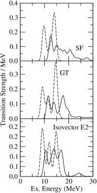
Figure 1: Isovector E2, SF and GT transition strengths for ²⁰Ne. Both the exact SM (solid curve) and RPA (dashed curve) distributions have been smoothed with a Gaussian of width 0.7 MeV to facilitate comparison.

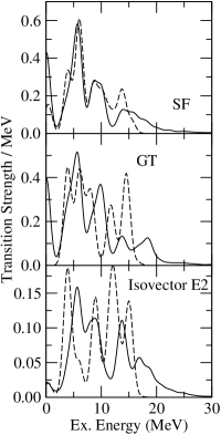
Figure 2: Same as in Fig. 1 for ²¹Ne.

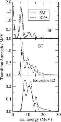
Figure 3: Same as in Fig. 1 for ²²Na.

Table 1: Total strength $S_{0}$, centroid $\bar{S}$, and width $\Delta S$ for isovector E2 transition operator. The nuclei have been grouped into even-even, odd-odd and odd-A.

	$S_{0}$		$\bar{S}$ (MeV)		$\Delta S$ (MeV)
Nucleus	SM	RPA	SM	RPA	SM	RPA
20Ne	0.98	1.15	14.53	11.92	3.47	2.44
22Ne	2.37	1.86	8.15	7.70	5.85	4.25
24Mg	1.88	1.96	14.40	11.86	4.09	2.46
28Si	2.28	1.96	14.35	13.41	4.29	1.93
36Ar	1.38	1.34	12.49	11.01	4.24	3.56
44Ti	2.15	1.90	8.23	6.68	2.86	1.98
22Na	1.60	1.69	11.67	10.44	4.37	2.61
24Na	2.07	2.09	9.82	8.21	6.26	4.14
46V	2.32	3.00	7.96	6.62	4.17	1.97
21Ne	1.39	1.43	10.52	9.41	5.66	4.27
25Mg	2.28	2.20	11.48	9.47	6.21	4.41
29Si	2.52	2.20	11.61	10.21	5.68	4.25

Table 2: Same as in Table 1 for SF transition operator.

	$S_{0}$		$\bar{S}$ (MeV)		$\Delta S$ (MeV)
Nucleus	SM	RPA	SM	RPA	SM	RPA
20Ne	1.05	1.23	17.10	12.26	4.38	1.95
22Ne	3.53	4.44	11.40	8.82	4.32	2.37
24Mg	4.15	4.78	13.22	10.17	4.48	1.97
28Si	5.82	5.20	12.75	11.62	4.34	1.89
36Ar	2.68	2.70	14.53	11.17	3.69	2.88
44Ti	2.56	3.32	9.98	7.86	2.56	1.55
22Na	8.57	5.78	5.01	6.67	5.22	3.49
24Na	10.06	7.66	5.83	7.05	5.48	3.19
46V	5.44	7.68	8.76	6.40	2.51	2.34
21Ne	4.02	3.54	7.50	7.62	5.92	3.95
25Mg	6.94	6.33	9.19	8.47	5.73	3.36
29Si	8.42	8.47	9.38	7.86	5.07	4.45

Table 3: Same as in Table 1 for GT transition operator.

	$S_{0}$		$\bar{S}$ (MeV)		$\Delta S$ (MeV)
Nucleus	SM	RPA	SM	RPA	SM	RPA
20Ne	1.05	1.33	16.32	12.53	4.35	2.42
22Ne	3.87	4.85	12.00	9.37	4.48	3.16
24Mg	4.26	4.85	14.46	11.74	4.24	2.42
28Si	6.65	5.70	15.19	13.77	3.59	1.88
36Ar	2.74	2.79	14.85	12.09	3.45	2.99
44Ti	3.03	3.74	10.12	8.42	2.86	2.43
22Na	5.51	5.47	9.96	9.28	4.35	3.18
24Na	7.43	7.71	10.32	9.29	4.87	3.48
46V	10.60	7.85	4.93	8.15	4.37	2.28
21Ne	4.25	3.55	7.87	8.67	5.97	3.98
25Mg	7.12	6.76	11.02	10.00	6.05	4.21
29Si	9.42	8.63	12.28	10.39	5.41	4.99

To summarize the results in this section, we have compared the SM and RPA distribution strengths for isovector E2, SF and GT transition operators. We found in general good agreement for the total strength in several nuclei. While less satisfactory, the centroids and widths of the distributions are still close. As a general feature however, the RPA distributions are smaller in width and lower in energy than the SM results.

III.3 Results for isoscalar quadrupole response

This section presents comparison between the SM and RPA distribution strength for the isoscalar quadrupole transition operator. The main difference with respect to the other transitions investigated in this paper is that the collective strength lies very low in energy, for realistic Hamiltonians have a strong attractive isoscalar quadrupole-quadrupole component.

We considered again for comparison the same nuclides investigated previously, and we plot the SM and RPA distributions in figures 4-6. Characteristics of the distributions for several other nuclei are given in table 4. In contrast with the results in Sec. III.2, we find a large discrepancy between the total strengths in RPA and SM, especially for even-even nuclei.

Figure 4 shows that, if one ignores the low energy transitions, one obtains again a reasonable agreement between the SM and RPA distributions. Similar features encountered for other transitions appear, that is a lower energy centroid and smaller width of the RPA distribution with respect to SM.

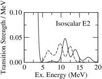
Figure 4: Isoscalar E2 transition strengths for ²⁰Ne. The SM (solid curve) and RPA (dashed curve) distributions have been smoothed with a Gaussian of width 0.7 MeV. The large collective peak at low but nonzero excitation energy for the SM is absent in the RPA; see text for discussion.

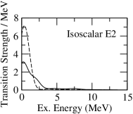
Figure 5: Same as Fig. 4 for ²¹Ne.

Table 4: Same as in Table 1 for isoscalar E2 transition operator.

	$S_{0}$		$\bar{S}$ (MeV)		$\Delta S$ (MeV)
Nucleus	SM	RPA	SM	RPA	SM	RPA
20Ne	7.86	0.19	2.12	9.81	1.92	2.30
22Ne	9.36	0.89	2.01	5.52	2.19	2.79
24Mg	12.57	0.51	2.13	7.99	2.09	2.75
28Si	12.04	0.56	2.51	9.88	2.33	2.33
36Ar	7.17	0.23	2.42	9.57	1.91	2.74
44Ti	10.87	1.50	1.73	3.99	1.73	1.70
22Na	9.53	7.49	1.47	1.27	2.63	1.82
24Na	8.81	6.33	2.10	1.81	2.85	1.88
46V	15.21	15.20	1.62	0.87	1.94	1.63
21Ne	8.74	13.27	1.53	0.64	2.82	1.35
25Mg	10.71	12.49	2.25	1.08	2.66	1.62
29Si	9.70	1.38	2.72	4.66	2.62	4.25

As for the relative good agreement for odd-odd and odd-$A$ nuclei, we have to point out that most of the RPA strength is concentrated in the lowest energy state which, as already noted, appears just as an artifact of our approach (restriction to real numbers). A full treatment of rotations by inclusion of complex numbers would shift these ‘soft-mode’ states to zero modes, that is, degenerate with respect to the ground-state, and we would expect the odd-odd and odd-$A$ cases to then resemble the even-even cases: missing the low-energy collective strength. (Note that qualitatively the results for ²⁹Si, for which we obtain the correct number of zero RPA modes, are similar to the even-even nuclei.) Conversely, we can turn around these results into a hypothesis: that the missing low-lying collective strength in even-even nuclides are due to incomplete symmetry restoration, and that the missing strength resides in the RPA ground state. The fact that the missing strength shows up in soft modes that arise as artifacts of our computational methods bolsters this hypothesis. For the interested reader, more details can be found in the next section.

III.4 “Missing strength” and broken symmetries

In this section we provide further evidence supporting our hypothesis that the low-lying collective strength is missing due to incomplete symmetry restoration in the RPA, and a significant fraction of the RPA strength gets absorbed in a ground state to ground state transition.

Our first test of incomplete symmetry restoration is the comparison of the transition strength for spherical and deformed HF solutions. While the proton-neutron interaction induces deformation in the HF Slater determinant for ²⁸Si, it is possible nevertheless to force a transition to a spherical HF state (both protons and neutrons filling the $d_{5/2}$ orbits) by increasing the gap between the $d_{5/2}$ single particle energy and the other single-particle states. The above-reported values for ²⁸Si use the USD value of $\epsilon(d_{5/2})=-3.94$ MeV, which yields a deformed HF state. In addition we computed ²⁸Si at $\epsilon(d_{5/2})=-5.64$ MeV and $-5.74$ MeV. At $-5.64$ MeV the HF state is still deformed while at $-5.74$ MeV the HF state is spherical. (Actually, for these values of $\epsilon(d_{5/2})$ there exist both spherical and deformed locally stable HF solutions, but at $-5.64$ MeV the deformed state has a slightly lower HF energy while at $-5.74$ MeV the spherical state has the lowest HF energy. Thus this is a first order ‘phase transition’ as described in section 4 of thouless61 . The so-called collapse or breakdown of RPA, readily seen in toy models such as the Lipkin model ring , only occurs when one has a second order ‘phase transition,’ when one has only one stable HF solution. In other words, our RPA calculations do not collapse at the transition point.)

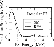
Figure 6: Same as Fig. 4 for ²²Na.

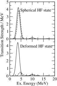
Figure 7: ²⁸Si: Isoscalar E2 for deformed and spherical HF state.

Figure 7 shows small difference in the SM strength distribution in contrast with a dramatic change for RPA. The difference between the $d_{5/2}$ single-particle energies in the two cases is small and one can follow a smooth change for all observables in the SM; we have therefore no reason to suspect any fundamental difference in the structure of the states. Note however that, when the HF state is spherical, the low lying states are correctly described in the RPA, the reason why the RPA was successful in describing low lying collectivity in closed shell nuclei; but note also that the high-lying part of the strength is not correctly described. In contrast, when the HF state is deformed, the RPA strength distribution changes dramatically, even through the SM strength distribution does not: the low-lying strength vanishes, but the high-lying strength is approximately correct.

As a second test, we compare the total strength $S_{0}$ and the energy-weighted sum rule $S_{1}$ computed in different ways.

Table 5 presents the total strength $S_{0}$ for a transition operator $F$, where $F$ is either the spin-flip operator or isoscalar E2 operator. The columns labled ‘SM’ are the exact shell model results, for which $S_{0}=\langle 0|F^{2}|0\rangle=\sum_{\nu}|\langle\nu|F|0\rangle|^{2}$. Of course, for the shell model both methods yield the same result. The columns RPA-X and RPA-$\Sigma$ correspond to equivalent methods for the RPA. RPA-X is the expectation value $\langle RPA|F^{\dagger}F|RPA\rangle$ as laid out in johnson2002 , where we showed that the RPA expectation value was often a reasonable approximation to the shell model result, though not always as seen for some of the spin-flip cases. RPA-$\Sigma$ is the sum $\sum_{\nu}|\langle\nu|F|RPA\rangle|^{2}$, where the sum is only to excited states as g.s.-to-g.s. transitions are difficult to define in RPA.

The horizontal lines in Table 5 segregate even-even nuclei with deformed HF states, even-even spherical nuclei, odd-odd nuclei, and odd-A nuclei. Keep in mind that for the latter two groups we do not get all the true zero modes (because we restricted the Slater determinant to real single-particle wavefunctions), but at least one zero mode is replaced by a soft mode, except for the case of ²⁹Si which does have all the expected zero modes.

What do we learn from Table 5? We draw the reader’s attention to the isoscalar E2 strength in deformed even-even-nuclides, and in ²⁹Si, all of which have the expected number of exact zero modes. Here the summed RPA strength (RPA-$\Sigma$) is dramatically and consistently smaller than either the exact SM result, or the expectation value RPA-X. By way of contrast, the nuclides with spherical HF states and thus no zero modes, or those who have soft modes rather than zero modes, have summed RPA strength in reasonable accord with the SM total strength. Furthermore the RPA expectation value of $Q\cdot Q$ also agrees with the SM total strength, which suggests to us that some of the missing RPA strength is in g.s. to g.s. transitions. This line of reasoning is weakened by the poor reliability of the RPA expectation value, as discussed in johnson2002 and as seen in the spin-flip values, which take on unphysical negative values for spherical nuclei.

Table 5: Comparison total strength $S_{0}$ as computed in the shell model (SM), by taking the expectation value of an observable (RPA-X), and by summing the RPA strengths directly (RPA-$\Sigma$); see text for more details. The horizontal lines separate even-even deformed nuclei, even-even spherical nuclei, odd-odd and odd-A. Notation on ²⁸Si: ^† indicates $\varepsilon_{d5/2}=-5.74$ MeV and a spherical HF state.

	SF			Isoscalar E2
Nucleus	SM	RPA-X	RPA-$\Sigma$	SM	RPA-X	RPA-$\Sigma$
20Ne	1.05	1.34	1.23	7.86	8.17	0.19
22Ne	3.52	1.94	4.44	9.36	9.98	0.89
24Mg	4.15	5.53	4.78	12.57	12.52	0.51
36Ar	2.68	2.90	2.70	7.17	7.66	0.23
28Si	5.82	5.13	5.20	12.04	13.77	0.56
28Si†	9.07	-5.22	12.53	7.95	7.50	6.86
22O	5.04	-0.60	6.31	2.71	2.75	2.36
24O	5.17	-1.07	6.24	1.88	1.92	1.57
22Na	8.57	7.64	5.78	9.53	9.92	7.49
24Na	10.06	6.97	7.66	8.81	9.61	6.33
21Ne	4.02	1.77	3.54	8.74	8.69	13.27
25Mg	6.94	1.52	6.33	10.71	12.34	12.49
29Si	8.42	5.77	8.47	9.70	11.67	1.38

Therefore, to further dissect this issue, in Table 6 we consider the energy-weighted sum rule $S_{1}$. The SM value is $\sum_{\nu}(E_{\nu}-E_{0})|\langle\nu|F|0\rangle|^{2}$. The RPA value is $\sum_{\nu}\Omega_{\nu}|\langle\nu|F|{\rm RPA}\rangle|^{2}$, while the HF value is $\frac{1}{2}\langle{\rm HF}|[F,[H,F]|{\rm HF}\rangle$ (for technical reasons, discussed in the Appendix, we can only compute this for even-even nuclei).

For nuclei with spherical HF states, that is, no zero modes, the RPA $S_{1}$ and the HF value are identical; this is the usual theorem regarding the energy weighted-sum rule. For nuclei with deformed HF states, and thus with zero modes, the RPA and HF values differ, a small amount for isovector E2 and dramatically for isoscalar E2. (We also computed but do not show values for the spin-flip operator; the results are similar to isovector E2, although with an even smaller contribution from the zero modes.) Overall these results are consistent with our hypothesis that low-lying strength is subsumed into the RPA ground state due to incompletely restoration of a broken symmetry; the difference is larger for isoscalar E2 because of the large strength at low energy.

Table 6: Comparison of energy-weighted sum rule $S_{1}$ as computed in the shell model (SM), taking the weighted sum of RPA strengths (RPA), and taking the HF expectation value of a double-commutator (HF); see text for more details. Notation on ²⁸Si, same as for Table 5.

	Isovector E2			Isoscalar E2
Nucleus	SM	RPA	HF	SM	RPA	HF
20Ne	14.27	13.74	13.74	16.63	1.82	7.43
22Ne	19.28	14.34	14.40	18.84	4.92	10.51
24Ne	21.89	14.89	15.06	20.87	8.42	11.99
24Mg	27.09	23.28	23.28	26.71	4.08	14.87
36Ar	17.24	14.72	14.72	17.32	2.21	8.64
28Si	32.66	26.22	26.22	30.22	5.58	17.67
28Si†	40.13	35.76	35.76	34.31	28.26	28.26
22O	11.46	8.56	8.56	11.46	8.56	8.56
22O	10.42	7.99	7.99	10.42	7.99	7.99

IV conclusions

The purpose of this paper was to investigate the reliability of the RPA for calculating transition strengths in nuclei. To accomplish this we have computed the RPA and shell model strength distributions in the same $0\hbar\omega$ shell model space.

The comparison between RPA and SM showed two different results, depending upon the nature of transitions. Thus, we found that when the strong collectivity lies at high energies, such as isovector E2, SF and GT transitions, the RPA and SM are in reasonable agreement. When the transitions lie at low energies however, the agreement is poor. We presented evidence that the problem arises from an incomplete restoration of the symmetries broken by the mean-field; for low-lying transitions we propose that significant part of the transition strength is subsumed into the RPA ground state. Future work should directly investigate ground-state to ground-state transitions in the RPA. (These are also needed for ground state moments, such as magnetic dipole or electric quadrupole, of odd-A nuclides.) Finally, we also have found, both analytically and numerically, that the standard lore regarding the RPA energy-weighted sum rule Eq. (13) does not hold if an exact symmetry is broken, particularly if the centroid of the transition strength is very low in energy.

This paper also marks a final stage within a larger project to test the reliability of the HF+RPA for a global microscopic theory of nuclear properties stetcu2002 ; johnson2002 . We conclude that HF+RPA is a good starting point for such a task, but because of occasional failures future work should investigate Hartree-Fock-Bogoliubov +QRPA and extensions such as renormalized RPA, self-consistent RPA, etc., (see Ref. ring as well as the bibliographies of stetcu2002 ; johnson2002 ) and the second RPA, which has been shown to differ significantly from the standard RPA in its description of E2 giant resonances of ¹⁶O secondRPA . Our work suggests an important and specific test of any such “improvement” to RPA: the description of low-lying collective strength, such as isoscalar E2, which is sensitive to restoration of the rotational symmetry broken by a deformed mean-field state.

*

Appendix A The energy-weighted sum rule, revisited

In Table 6 we saw a discrepancy between two ways to compute the energy-weighted sum rule,

$$S_{1}^{HF}=\frac{1}{2}\sum_{M}(-1)^{M}\langle\mathrm{HF}|[F_{K,-M},[H,F_{KM}]]|\mathrm{HF}\rangle$$ (14)

and

$$S_{1}^{RPA}=\sum_{\nu}\sum_{M}\Omega_{\nu}\left|\langle\nu|F_{KM}|\mathrm{RPA}\rangle\right|^{2}.$$ (15)

In textbooks ring one finds “proof” that $S_{1}^{HF}=S_{1}^{RPA}$, which is often stated that RPA preserves the energy-weighed sum rule. In this Appendix we revisit the proof, with special attention to zero modes that arise from broken exact symmetries, and we find that instead $S_{1}^{HF}=S_{1}^{RPA}+$ a term that arises from zero modes.

Suppose we have a broken symmetry, such as rotational invariance. The Hartree-Fock state is deformed and has a particular orientation, but the Hartree-Fock energy is independent of the orientation. This shows up in the RPA matrix equation (8) as a zero-frequency mode. For $\Omega>0$ one has the normalization $\vec{X}^{2}-\vec{Y}^{2}=1$ but this normalization is impossible for $\Omega=0$. Instead one introduces collective coordinates $\vec{Q}_{\nu}$ and conjugate momenta $\vec{P}_{\nu}$ring ; weneser , which satisfy

$$\textbf{A}\vec{P}_{\nu}-\textbf{B}\vec{P}^{*}_{\nu}=iM_{\nu}\Omega^{2}_{\nu}\vec{Q}_{\nu},$$

$$\textbf{A}\vec{Q}_{\nu}-\textbf{B}\vec{Q}^{*}_{\nu}=-\frac{i}{M_{\nu}}\vec{P}_{\nu}.$$ (16)

Here $M_{\nu}$ is a constant, interpretable as mass or moment of inertia fixed by the normalization of $P,Q$:

$$\vec{Q}^{*}_{\lambda}\cdot\vec{P}_{\nu}-\vec{Q}_{\lambda}\cdot\vec{P}^{*}_{\nu}=i\delta_{\lambda\nu}.$$ (17)

Note that if A and B are real, then $X$, $Y$ are real, but of necessity $P$ and $Q$ are complex (one is real and the other imaginary). With these zero-mode frequencies one must supplement the quasiboson operators $\beta,\beta^{\dagger}$ in Eq. (7) with the generalized coordinate and momentum operators ${\cal Q},{\cal P}$.

Because of the expansion (11) one can use the definitions (9), (10), and able to use $A$ and $B$ to write $S_{1}^{HF}$ as

$$\sum_{M}\sum_{mi,nj}\left(A_{mi,nj}f_{mi}^{M}f_{nj}^{M}-(-)^{M}B_{mi,nj}f_{mi}^{M}f_{nj}^{-M}\right)$$

The matrices $A$ and $B$ can be written in terms of particle hole amplitudes $X$ and $Y$, and the canonical momentum operators associated with broken symmetries

$$A=X\Omega X^{\dagger}+Y^{*}\Omega Y^{T}+PM^{-1}P^{\dagger},$$ (18)

$$-B=X\Omega Y^{\dagger}+Y^{*}\Omega X^{T}-PM^{-1}P^{T}.$$ (19)

Substitution and some algebra yields

$$S_{1}^{HF}=S_{1}^{RPA}+$$

$$\sum_{M}\sum_{\mu(\Omega_{\mu}=0)}\frac{1}{2M_{\mu}}\left|f^{M}\cdot P_{\mu}-(-)^{M}f^{-M}\cdot P_{\mu}^{*}\right|^{2}$$

Although we do not show it, one can write the right-hand side as a double-commutator of boson operators.

As further motivation, one can start from Eq. (12) and write the contribution from a single frequency to the RPA energy-weighted sum rule as

$$S_{1}^{RPA}(\mu)=\Omega_{\mu}\sum_{M}|f^{M}\cdot X^{\mu}+(-1)^{M}f^{-M}\cdot Y^{\mu}|^{2}.$$ (21)

Even if $\mu$ is not a zero mode, one is free to transform to collective coordinates and momenta ring ,

$$X^{\mu}=\sqrt{\frac{M_{\mu}\Omega_{\mu}}{2}}Q_{\mu}-i\sqrt{\frac{1}{2M_{\mu}\Omega_{\mu}}}P_{\mu}$$ (22)

$$Y^{\mu}=-\sqrt{\frac{M_{\mu}\Omega_{\mu}}{2}}Q_{\mu}^{*}+i\sqrt{\frac{1}{2M_{\mu}\Omega_{\mu}}}P_{\mu}^{*}.$$ (23)

Inserting into (21) and letting $\Omega_{\mu}\rightarrow 0$, there is a finite remainder exactly equal to the rightmost term of (A). It is of course surprising to find contribution to the energy-weighted sum rule from ‘zero excitation energy’. But we remind the reader that the RPA zero modes are continuous states arising from broken symmetries in the mean-field solution, while the discrete states are quantized harmonic oscillations about the HF Slater determinant. Part of the challenge of RPA is that continuous modes clearly cannot be treated on the same footing as the discrete states.

We find numerically that the discrepancy in Table 6 is given exactly by the last term in Eq. (A). Our interpretation of Table 6 and Eq. (A) is missing strength that goes into g.s.-to-g.s. transitions, due to incomplete symmetry restoration. Undoubtedly more work remains, but we hope our results act to inspire further careful investigation. For example, for some transition operators there is no or very small contribution from the zero modes even for nuclides with deformed HF states; this seems to be associated with transitions with high-lying giant resonances, again consistent with our interpretation of incomplete restoration of symmetries and low-lying strength being subsumed into the RPA ground state.

Finally, we wish to discuss the general rule

$$\sum_{\nu}(E_{\nu}-E_{\mu})|\langle\mu|F|\nu\rangle|^{2}=\frac{1}{2}\langle\mu|[F,[H,F]]|\mu\rangle.$$ (24)

Eq. (24) is true for any true eigenstate $|\mu\rangle$, and so holds for full shell-model calculations. But the HF state is not an eigenstate, and so one cannot use the Lanczos moment method described in Section II.2. Instead, we take the HF state and project onto a vector in the basis of shell-model states (because shell-model basis states have good $J_{z}$, the projection can only be done easily for even-even nuclides); both $H$ and $F_{KM}$ are matrices in the restricted model space and we compute directly $(HF-FH)|\mathrm{HF}\rangle$ and dot that vector onto $F|\mathrm{HF}\rangle$. One must sum over all shell-model states with intermediate values of $J_{z}$, a tedious but necessary task for computing $S_{1}^{HF}$.

- (1) P. Ring and P. Shuck, The nuclear many-body problem, 1st ed. (Springer-Verlag, New York 1980).
- (2) G. E. Brown and A. M. Green, Nucl. Phys. 75, 401 (1966); W.C. Haxton and C. W. Johnson, Phys. Rev. Lett. 65, 1325 (1990); E. K. Warburton, B. A. Brown, and D. J. Millener, Phys. Lett. B 293, 7 (1992).
- (3) T. T. S. Kuo, J. Blomqvist, and G. E. Brown, Phys. Lett. 31B, 93 (1970).
- (4) P. von Neumann-Cosel et. al., Phys. Rev. Lett. 82, 1105 (1999).
- (5) N. Ullah and D. J. Rowe, Phys. Rev. 188, 1640 (1969).
- (6) J. Blomqvist and T. T. Kuo, Phys. Lett. 29B, 544 (1969).
- (7) W. W. True, C. W. Ma, and W. T. Pinkston, Phys. Rev. C 3, 2421 (1971).
- (8) D. J. Rowe and S. S. M. Wong, Phys. Lett. 30B, 147 (1969); Nucl. Phys. A153, 561 (1970).
- (9) K. Goeke and J. Speth, Ann. Rev. Nucl. Part. Sci. 32, 65 (1982).
- (10) A. M. Oros, K. Heyde, C. De Coster, and B. Decroix, Phys. Rev. C 57, 990 (1988).
- (11) V.G. Soloviev, A.V. Sushkov, N.Yu. Shirikova, and N.Lo Iudice, J. Phys. G 25, 1023 (1999); N. Lo Iudice, A.V. Sushkov, and N. Y. Shirikova, Phys. Rev. C 64, 054301 (2001).
- (12) S.M. Grimes et. al, Phys. Rev. C 53, 2709 (1996).
- (13) J. E. Wise et. al, Phys. Rev. C 31, 1699 (1985).
- (14) J.U. Nabi and H.V. Klapdor-Kleingrothaus, Acta Phys. Polonica B 30, 825 (1999); Atom. Data Nucl. Data 71, 149 (1999)
- (15) I. Hamamoto, H. Sagawa, and X.Z. Zhang, Phys. Rev. C 55, 2361 (1997);Phys. Rev. C 56, 3121 (1997); P. Urkedal, X.Z. Zhang, and I. Hamamoto, Phys. Rev. C 64, 054304 (2001).
- (16) I. Stetcu and C.W. Johnson, Phys. Rev. C 66, 034301 (2002).
- (17) O. Civitarese and M. Reboiro, Phys. Rev. C 57, 3062 (1998).
- (18) S. Stoica, I. Mihut, and J. Suhonen, Phys. Rev. C 64, 017303 (2001).
- (19) J. Engel, S. Pittel, M. Stoitsov, P. Vogel, and J. Dukelsky, Phys. Rev. C 55, 1781 (1997).
- (20) B. Lauritzen, Nucl. Phys. A489, 237 (1998).
- (21) O. Civitarese, H. Müller, L. D. Skouras, and A. Faessler, J. Phys. G. 17, 1363 (1991).
- (22) L. Zhao and B. A. Brown, Phys. Rev. C 47, 2641 (1993).
- (23) N. Auerbach, G. F. Bertsch, B. A. Brown, and L. Zhao, Nucl. Phys. A556, 190 (1993).
- (24) G.E. Brown and M. Bosterli, Phys. Rev. Lett. 3, 427 (1959).
- (25) A. R. Edmonds, Angular Momentum in Quantum Mechanics, (Princeton University Press, Princeton, 1960).
- (26) R. R. Whitehead,A. Watt, B. J. Cole, and I. Morrison, Adv. Nucl. Phys. 9, 123 (1977).
- (27) E. Caurier, A. Poves, and A.P. Zuker, Phys. Lett. B252, 13 (1990); Phys. Rev. Lett 74, 1517 (1995).
- (28) Kris L.G. Heyde, The nuclear shell model (Springer-Verlag, Berlin, 1990).
- (29) D.J. Thouless, Nucl. Phys. 22, 78 (1961).
- (30) G.F. Bertsch and K. Hagino, Phys. Atom. Nucl. 64,588 (2001) [arXiv:nucl-th/0006032]
- (31) C. W. Johnson and I. Stetcu, Phys. Rev. C 66, 064304 (2002).
- (32) E. R. Marshalek and J. Weneser, Ann. Phys. 53, 569 (1969).
- (33) B.H. Wildenthal, Prog. Part. Nucl. Phys. 11, 5 (1984).
- (34) T.T.S. Kuo and G.E. Brown, Nucl. Phys. A114, 235 (1968); A. Poves and A.P. Zuker, Phys. Rep. 70, 235 (1981).
- (35) M. Tohyama, Phys. Rev. C 58, 2603 (1998).