Abstract

The exclusive charge exchange reaction $pD\to n(pp)$ at intermediate and high energies is studied within the Bethe-Salpeter formalism. The final state interaction in the detected $pp$ pair at nearly zero excitation energy is described by the ${}^{1}S_{0}$ component of the Bethe-Salpeter amplitude. Results of numerical calculations of polarization observables and differential cross-section persuade that, as in the non-relativistic case, this reaction (i) can be utilized as a “relativistic deuteron polarimeter” and (ii) delivers further information about the elementary nucleon-nucleon charge-exchange amplitude.

I Introduction

The investigation of polarization observables in electromagnetic and hadronic processes at high energies provides refinement of the information about strong interaction at short distances and the relevant reaction mechanisms. Accordingly, the experimental study of processes with polarized particles becomes more and more important. Experiments with deuteron targets or beams alexa ; kox0 ; preliminar ; cosy_proposal are particularly interesting, since the deuteron serves as a unique source of information on neutron properties at high transferred momenta; the knowledge of which allows, e.g. to check a number of QCD predictions and sum rules. For example, for an investigation of the $NN$ interaction in the deuteron at short distances, the three deuteron form factors (magnetic, electric and quadrupole) have to be determined. In the elastic $eD$ scattering with unpolarized particles one can measure only two independent quantities, e.g. the magnetic form factor and the deuteron function $A(Q^{2})$, the latter being a kinematical combination of all three form factors. Even these two quantities reveal an important information about the quark physics and dynamics at short distances as demonstrated, for instance, in recent measurements alexa at TJNAF. However, for a full determination of the deuteron form factors separately, one needs measurements with polarized particles. For instance, measurements of the tensor analyzing power $T_{20}$ of recoil deuterons in elastic $eD$ scattering allow for a determination of the charge form factor $G_{c}$ at high transferred momenta. Namely the charge form factor is very sensitive to details of the $NN$ interaction kox0 ; preliminar ; gross and, besides information about short range correlations in the deuteron, the investigation of $G_{c}$ may essentially constrain the theoretical models applied in this area. However, in spite of the fact that the electromagnetic processes are considered as the cleanest ones, in such reactions one probes mainly the quark structure of the target, leaving almost untouched the physics connected with gluon degrees of freedom. In this context, hadron deuteron processes can be considered as complementary tool in investigating phenomena at short distances and also as a source of unique information unavailable in electromagnetic reactions, such as nucleon resonances, checking non-relativistic effective models, $NN$ potentials etc.

Experimental and theoretical investigations of the proton-deuteron processes at intermediate and high energies have started some decades ago by studying elastic $pD$ scattering elsatic , exclusive and inclusive break-up reactions inclusive ; cosy with the goal of determining the the details of the deuteron wave function at short distances and the relevant reaction mechanisms. Note, that in elastic backward $pD$ processes it is possible to determine completely the reaction amplitude by measuring a full set of polarization observables (see, e.g., rekalo ; ladygin ; ourprc ). Hence, as in the electromagnetic processes one needs to measure different polarizations of the recoil deuteron.

Since such polarization observables can be studied only by an additional secondary scattering of the reaction products, e.g., inside a polarimeter, it is obvious that second process must possess a high enough cross section to assure a good efficiency of the polarimeter. Traditionally, at low energies one uses the process ${\rm{}^{3}He}\,(D,p)\,{\rm{}^{4}He}$ grub , while for relativistic energies the elastic $Dp$ scattering serves as polarimeter bald . Bugg and Wilkin wil1 proposed to use as an efficient deuteron polarimeter the process $p{\vec{D}}\to n(pp)$, where the final $pp$ pair is detected with very low excitation energy (see also ref. polder ). It has been argued that at low excitation energies and low transferred momenta the process $p{\vec{D}}\to n(pp)$ is determined by the elementary $pn$ charge-exchange of the incoming proton with the neutron in the deuteron, whereas the second proton acts merely as a spectator. In this case, the detected $pp$ pair can be considered to be in the ${}^{1}S_{0}$ final state. Within the non-relativistic spectator mechanism, a significant value of the tensor analyzing power $T_{20}$ and a vanishing vector analyzing power were predicted wil1 . The corresponding cross section is rather large, so that the process $p{\vec{D}}\to n(pp)$ can be considered as a good tool for determining the deuteron tensor characteristics. Later detailed investigations  ishida ; moto ; wil2 ; kox of this process confirmed the previous theoretical predictions wil1 . The charge-exchange processes of this type have also been proposed for investigations of other processes with deuterons, e.g. $pp\to D\pi^{+}$ reactions bugg , $\Delta N$ systems kozi , $NN\pi$ systems, inelastic $({\vec{D}},{\vec{D}^{\prime}})$ reactions off heavy nuclei to study isoscalar transitions $\Delta T=0,\,\Delta S=1$ morlet etc. In addition, the reaction $p{\vec{D}}\to n(pp)$ may be interesting in investigations of the elementary $NN$ amplitude. As shown in ref. wil1 , this reaction can be used as a part of a complete set of experiments to determine completely the amplitude of charge-exchange reaction $pn\to np$ glagolev . One may also investigate the influence of the nuclear medium on the $NN$ amplitude heckman ; titov , or to study the double spin flip processes in quasi elastic scattering of deuterons from heavy nuclei ishida .

The direct consequence of these facts is that nowadays the interest in investigations of charge-exchange processes does not abate. For example, at the cooler synchrotron COSY in FZ Jülich a program to study of similar processes at relativistic energies has already started cosy_proposal ; cosy and a detailed investigation of polarization observables is envisaged. Inspired by this, in previous work nashyaf we investigated the process $p{\vec{D}}\to n(pp)$ within the impulse approximation. The goal of the present paper is to consider the charge-exchange reaction at relativistic energies, as accessible at COSY and upgraded Dubna accelerator by (i) taking into account the effects of final state interaction, (ii) to check whether in this case the non-relativistic predictions wil1 hold and (iii) whether the reaction still can be regarded as a deuteron polarimeter tool and/or as complementary source of an experimental determination of the elementary charge-exchange partial amplitudes. We propose a covariant generalization of the spectator mechanism wil1 based on the Bethe-Salpeter (BS) formalism and on a numerical solution of the BS equation with a realistic one-boson exchange kernel solution ; parametrization . Our amplitude of the process in an explicitly covariant form allows for a determination of any polarization observables. Nevertheless, here we focus on calculations of the cross section and the tensor analyzing power $T_{20}$ for kinematical conditions as relevant for experiments at COSY. Vector analyzing powers of the deuteron are strictly equal to zero in our case, since we consider the ${}^{1}S_{0}$ NN final state. The corresponding expressions are quite lengthy, so we do not present an explicit comparison with the non-relativistic formulae, nevertheless, the final results are written in a form as close as possible to the non-relativistic case. We are going to compare our results, computed at non-relativistic energies, with corresponding data and corresponding non-relativistic calculations wil2 thus demonstrating that our formulae hold in the non-relativistic limit as well, as it should be. We adopt for the process $p{\vec{D}}\to n(pp)$ with a slowly moving, small-excitation energy $pp$ pair the same mechanism as in wil1 , i.e., the process is treated, in the deuteron center of mass, as a charge-exchange between the incoming proton and internal neutron with the second proton as a spectator. The resulting $pp$ pair is supposed to be detected solely in the ${}^{1}S_{0}$ state. Particular attention is paid to the pure impulse approximation, where the final state interaction in the $pp$ pair is, for the time being, disregarded. Within the impulse approximation we study systematically peculiarities of the reaction to find proper kinematical conditions where the supposed mechanism is adequate and to fix the choice of input parameters. Then the final state interaction in the ${}^{1}S_{0}$ state is taken into account by solving the inhomogeneous BS equation in the one-iteration approximation, which allows one to numerically compute the corresponding partial amplitudes. The effects of final state interaction are found to be substantial and essentially improve the agreement with data. Methodological prediction for the COSY kinematics will be presented as well.

This paper is organized as follow. In Sect. II kinematics and notation are introduced. A short review of the spin structure of the amplitude $\displaystyle\frac{1}{2}+1\to\displaystyle\frac{1}{2}+0$ and definitions of polarization observables are presented. Sect. III deals with the invariant amplitude within the BS formalism and defines the corresponding BS wave functions. A reduction of the covariant form of the amplitude to the traditional form in the two dimensional spinor space is also performed in this section. In the next section IV a detailed study of relativistic impulse approximation and a comparison with data is given. In Sect. V the procedure of accounting for final state interaction in the continuum within the BS formalism is discussed. The total BS wave function for the ${}^{1}S_{0}$ configuration is presented, the corresponding numerical calculations of the cross section and tensor analyzing power and a comparison with the available experimental data is performed. Conclusions and summary may be found in Sect. VI. Some cumbersome expressions are relegated to the Appendices.

II Kinematics and notation

Since in the exclusive processes with three nucleons in the final state we are interested in studying correlations in the $pp$ pair we select those of them which, in the deuteron center of mass system, correspond to final states with one fast neutron and a slowly moving proton-proton pair, i.e. reactions of the type

$$p\,+\,\vec{D}\,=\,n+(p_{1}+p_{2}).$$ (1)

A peculiarity of the processes (1) is that the transferred momentum from the proton to the neutron is low, hence the main mechanism of the reaction can be described as a charge-exchange process of the incoming proton off the internal neutron, whereas the second proton in the deuteron remains merely as a spectator. As well known (see e.g. ref. diu ) the differential cross section of elementary charge-exchange process $pn\to np$ exhibits a sharp maximum at vanishing transferred momenta. Therefore, if the reaction (1) is indeed governed by a charge-exchange subprocess, then the resulting $pp$ pair will be detected with low total and relative momenta. Reactions of this kind can fairly well be distinguished from other processes. For relatively low initial energies, such reactions are quite well experimentally investigated. In Fig. 1, the diagram of such processes is schematically depicted. The following notations are adopted: $p=(E_{p},{\mbox{\bf p}})$ and $n=(E_{n},{\mbox{\bf n}})$ are the 4-momenta of the incoming proton and outgoing neutron, $P^{\prime}$ is the total 4-momentum of the $pp$ pair, which is a sum of the corresponding 4-momenta of detected protons, $p_{1}=(E_{1},{\mbox{\bf p}}_{1})$, $p_{2}=(E_{2},{\mbox{\bf p}}_{2})$, $P^{\prime}=p_{1}+p_{2}$. The invariant mass squared of the pair is $s_{f},~{}s_{f}=P^{\prime 2}=(2m+E_{x})^{2}$, where $m$ stands for the nucleon mass and $E_{x}$ for the excitation energy of the pair. Conform the supposed reaction mechanism, the excitation energy $E_{x}$ ranges to a few MeV, say $E_{x}=0-8$ MeV. At such low values of $E_{x}$, the main contribution in the final state of the $pp$ pair in the continuum comes from the ${}^{1}S_{0}$ configuration wil2 . In what follows all corrections from higher partial waves are neglected, however, we realize that for higher values of $E_{x}$ an increasing role of these corrections is expected.

Further, the Dirac spinors

$$u({\mbox{\bf p}},r)=\sqrt{m+\epsilon}\left(\begin{array}[]{c}\chi_{r}\\ \displaystyle\frac{({\mbox{\boldmath$\sigma$}}\cdot{\mbox{\bf p}})}{m+\epsilon}\chi_{r}\end{array}\right)$$ (4)

normalized as $\bar{u}(p)u(p)=2m$ are introduced. Then the differential cross section for the reaction (1) reads

$$d^{9}\sigma\,=\,\frac{1}{2\sqrt{\lambda(p,D)}}\,|M_{fi}|^{2}\,(2\pi)^{4}\delta(P_{f}-P_{i})\,\frac{d^{3}{\mbox{\bf n}}}{2E_{n}(2\pi)^{3}}\,\frac{1}{2}\prod\limits_{k=1}^{2}\frac{d^{3}{\mbox{\bf p}}_{k}}{2E_{k}(2\pi)^{3}},$$ (5)

where $\lambda(p,D)$ is the flux factor, $M_{fi}$ is the invariant amplitude and the statistical factor $1/2$ is due to two identical particles (protons) in the final state. By changing in eq. (5) the kinematical variables from the momenta ${\mbox{\bf p}}_{1,2}$ to the relative and total momenta of the pair and taking into account that there is no angular dependence in the ${}^{1}S_{0}$ configuration the cross section can be written as

$$d^{3}\sigma\,=\,\frac{1}{16\pi\sqrt{\lambda(p,D)}}\,\sqrt{1-\frac{4m^{2}}{s_{f}}}\,|M_{fi}|^{2}\,\frac{d^{3}{\mbox{\bf n}}}{2E_{n}(2\pi)^{3}}\,\frac{1}{2}.$$ (6)

Since our numerical solution of the Bethe-Salpeter equation has been obtained in the deuteron rest system all further calculations are performed in that. The quantization $z$ axis is chosen along the momentum p of the incoming proton; the $x$ and $y$ axes will be specified below. Changing the variables in (6) we arrive at

$$\frac{d^{2}\sigma}{dt\,ds_{f}}\,=\,\frac{1}{2}\frac{1}{64\pi\lambda(p,D)}\,\sqrt{1-\frac{4m^{2}}{s_{f}}}\,\int\frac{d\phi}{(2\pi)^{3}}\,|M_{fi}|^{2},$$ (7)

where $q=n-p$, $t=q^{2}$, $s_{f}=(D-q)^{2}$, and $\phi$ denotes the azimuthal angle of the final neutron. Further we consider only the case where the initial proton and the final neutron are unpolarized and the polarization density matrix of the initial deuteron, $\rho_{D}$, possesses an axial symmetry relative to the $z$-direction, i.e.

$$\rho_{D}=\frac{1}{3}\,{\bf 1}\,+\,p_{v}\,{\hat{T}}_{10}\,+\,p_{t}\,{\hat{T}}_{20},$$

where $p_{v}$ and $p_{t}$ are the vector and tensor polarization parameters, respectively. In this case the angular dependence upon $\phi$ in eq. (7) is trivial. Finally one has

$$\frac{d^{2}\sigma}{dt\,ds_{f}}\,=\,\frac{1}{2}\frac{1}{64\pi\lambda(p,D)}\,\sqrt{1-\frac{4m^{2}}{s_{f}}}\,\frac{1}{(2\pi)^{2}}\,|M_{fi}|^{2},$$ (8)

where the amplitude $|M_{fi}|^{2}$ can be computed at arbitrarily fixed value of $\phi$, e.g., $\phi=0$. The procedure of computing the amplitude $M_{fi}$ consists on several stages: (i) we analyze general spin structure in terms of a decomposition of $M_{fi}$ over a relevant independent set of spin variables with coefficients being invariant partial spin amplitudes of the process since all observables can be expressed via these partial amplitudes, (ii) the diagram in Fig. 1 is computed explicitly and the results for $M_{fi}$ are regrouped to obtain an expression in the same form as for the general decomposition of $M_{fi}$, (iii) from the direct comparison of the expression with the phenomenological form the partial spin amplitudes are found and the polarization observables computed.

By virtue of zero angular momentum of the final pair, the process (1) is of the type $1/2\,+\,1\,=\,1/2\,+\,0$, for which the symmetry restrictions leave only six independent (complex) partial amplitudes. The choice of their explicit representation depends upon the kinematical conditions of the attacked problem. One may choose the helicity representation, or the representation with a given spin projection for specific choices of the quantization axis etc. In this paper, we choose the following way to determine the partial amplitudes (see also keaton ): initial $|i\rangle$ and final $|f\rangle$ states of the system, besides other quantum numbers, are characterized by the spin projections on the $z$ axis; in the matrix element $M_{fi}$ this spin dependence is written explicitly by emphasizing in $|i\rangle$ and $|f\rangle$ the 3-polarization vector of the deuteron and the two-component Pauli spinors for nucleons. We introduce, in the deuteron center of mass, where ${\mbox{\bf D}}={\bf 0}$, the three basis vectors as follows

$${\mbox{\bf c}}=\frac{{\mbox{\bf p}}}{|{\mbox{\bf p}}|},\quad{\mbox{\bf b}}=\frac{[{\mbox{\bf p}}\times{\mbox{\bf n}}]}{|[{\mbox{\bf p}}\times{\mbox{\bf n}}]|},\quad{\mbox{\bf a}}=[{\mbox{\bf b}}\times{\mbox{\bf c}}].$$ (9)

Then the amplitude $M_{fi}$ can be represented in the form

$$M_{fi}\equiv{\cal T}_{r^{\prime}r}^{M}=[\chi_{r^{\prime}}^{+}]_{\alpha}\,\left({\cal M}_{\alpha\beta}\,{\mbox{\boldmath$\xi$}}_{M}\right)[\chi_{r}]_{\beta},\quad\alpha,\beta=1,2,$$ (10)

where $r^{\prime},r$ and $M$ are the spin projections for the neutron, proton and deuteron, respectively. The amplitude ${\cal M}_{\alpha\beta}$ is a vector in the coordinate space and a matrix in the spinor basis and consequently can be decomposed over the introduced basis vectors (9) and Pauli matrices $\sigma_{i}$ ($i=x,y,z$) as

$${\cal M}_{\alpha\beta} = i\,{\cal A}\,{\mbox{\bf b}}\,\delta_{\alpha\beta}+{\cal B}\,{\mbox{\bf b}}\,\,({\mbox{\boldmath$\sigma$}}\cdot{\mbox{\bf b}})_{\alpha\beta}+{\cal C}\,{\mbox{\bf a}}\,({\mbox{\boldmath$\sigma$}}\cdot{\mbox{\bf a}})_{\alpha\beta}+$$ (11)

$$+ {\cal D}\,{\mbox{\bf a}}\,({\mbox{\boldmath$\sigma$}}\cdot{\mbox{\bf c}})_{\alpha\beta}+{\cal E}\,{\mbox{\bf c}}\,({\mbox{\boldmath$\sigma$}}\cdot{\mbox{\bf a}})_{\alpha\beta}+{\cal F}\,{\mbox{\bf c}}\,({\mbox{\boldmath$\sigma$}}\cdot{\mbox{\bf c}})_{\alpha\beta}.$$

In eq. (10 ), ${\mbox{\boldmath$\xi$}}_{M}$ stands for the polarization vector of the deuteron in its center of mass system:

$$\begin{array}[]{ccc}{\mbox{\boldmath$\xi$}}_{+1}=-\displaystyle\frac{1}{\sqrt{2}}\,\left(\begin{array}[]{c}1\\ i\\ 0\end{array}\right),&\quad{\mbox{\boldmath$\xi$}}_{-1}=\displaystyle\frac{1}{\sqrt{2}}\left(\begin{array}[]{c}1\\ -i\\ 0\end{array}\right),&\quad{\mbox{\boldmath$\xi$}}_{0}=\left(\begin{array}[]{c}0\\ 0\\ 1\end{array}\right).\end{array}$$ (12)

Due to the use of the two-dimensional spin and 3-dimensional vector representation, eqs. (10) and (11) are not manifestly covariant. Nevertheless, such a representation of partial amplitudes is of most general form and valid in both relativistic and non-relativistic considerations. This may immediately be seen if one expresses in covariant matrix elements the polarization 4-vector of the deuteron $\xi_{M}$ (in any system of reference) via the 3-dimensional ${\mbox{\boldmath$\xi$}}_{M}$ as

$$\xi_{M}=\left[\frac{({\mbox{\bf D}}\cdot\mbox{\boldmath{$\xi$}}_{M})}{M_{D}},\,\mbox{\boldmath{$\xi$}}_{M}+{\mbox{\bf D}}\frac{({\mbox{\bf D}}\cdot\mbox{\boldmath{$\xi$}}_{M})}{M_{D}(E_{D}+M_{D})}\right],$$

and passes from the 4-spinors defined in eq. (4) to Pauli spinors $\chi_{r}$.

For convenience, the $y$ and $x$ axes are oriented along b and a, respectively. In this case the neutron azimuthal angle $\phi$ can be put equal to zero. The $z$ axis, as mentioned above, is parallel to c. The three variables, upon which the partial amplitudes ${\cal A},{\cal B},...{\cal F}$ depend, are chosen to be the total initial energy $s$, the transferred momentum $t$, and the invariant mass of the $pp$ pair $s_{f}$. These amplitudes are related with the spin amplitudes ${\cal T}_{r^{\prime}r}^{M}$ via the following expressions

$$\begin{array}[]{ll}{\cal A}=({\cal T}_{-\frac{1}{2}-\frac{1}{2}}^{1}+{\cal T}_{\frac{1}{2}\frac{1}{2}}^{1})/\sqrt{2},&\quad{\cal B}=-({\cal T}_{\frac{1}{2}-\frac{1}{2}}^{1}-{\cal T}_{-\frac{1}{2}\frac{1}{2}}^{1})/\sqrt{2},\\ {\cal C}=-({\cal T}_{\frac{1}{2}-\frac{1}{2}}^{1}+{\cal T}_{-\frac{1}{2}\frac{1}{2}}^{1})/\sqrt{2},&\quad{\cal D}=({\cal T}_{-\frac{1}{2}-\frac{1}{2}}^{1}-{\cal T}_{\frac{1}{2}\frac{1}{2}}^{1})/\sqrt{2},\\ {\cal E}={\cal T}_{\frac{1}{2}-\frac{1}{2}}^{0},&\quad{\cal F}={\cal T}_{\frac{1}{2}\frac{1}{2}}^{0}.\end{array}$$ (16)

Note that having computed the amplitudes ${\cal A},{\cal B},...{\cal F}$, all polarization observables for the process (1) can be found as proper combinations of these partial amplitude. So, if an operator ${\cal O}$ corresponds to a measurable physical quantity then its mean value is

$$\langle{\cal O}\rangle=6\frac{\mbox{Tr}\left({\cal M}\,{\cal O}\,{\cal M}^{+}\right)}{\mbox{Tr}\left({\cal M}\,{\cal M}^{+}\right)},$$ (17)

where the denominator corresponds to the cross section of the reaction (1) with unpolarized particles

$$\frac{1}{6}\mbox{Tr}\left({\cal M}{\cal M}^{+}\right)=\frac{1}{3}({\cal A}{\cal A}^{*}+{\cal B}{\cal B}^{*}+{\cal C}{\cal C}^{*}+{\cal D}{\cal D}^{*}+{\cal E}{\cal E}^{*}+{\cal F}{\cal F}^{*}).$$

For instance, the tensor analyzing power $\langle T_{20}\rangle$ is

$$\langle T_{20}\rangle = 6\frac{\mbox{Tr}\left({\cal M}\,{\hat{T}}_{20}\,{\cal M}^{+}\right)}{\mbox{Tr}\left({\cal M}\,{\cal M}^{+}\right)}$$ (18)

$$= \frac{\sqrt{2}}{\mbox{Tr}\left({\cal M}\,{\cal M}^{+}\right)}\,({\cal A}{\cal A}^{*}+{\cal B}{\cal B}^{*}+{\cal C}{\cal C}^{*}+{\cal D}{\cal D}^{*}-2\,[{\cal E}{\cal E}^{*}+{\cal F}{\cal F}^{*}]).$$

Note that the representation of the amplitude $M_{fi}$ by eqs. (10) and (11) holds if initial and final states can be described by wave functions (pure spin states), otherwise for mixed states the square of $M_{fi}$ must be averaged with the spin density matrices

$$\rho_{N}=\frac{1}{2}\,\sum_{r}|r\rangle\langle r|,\quad\rho_{D}=\frac{1}{3}\,\sum_{M}|M\rangle\langle M|.$$ (19)

An explicit covariant expression for the deuteron density matrix can be found in ref. ourphyslett . In the present paper the amplitudes ${\cal T}_{r^{\prime}r}^{M}$ and observables for the reaction (1) are evaluated within the BS formalism. It is worth noting that in theoretical considerations of high energy reactions with deuterons as target and two interacting nucleons in the final state (scattering or bound state) always, at least one of two-nucleon systems is moving, consequently Lorenz boost effects must be treated in a consistent way. In our opinion, the most appropriate approach for these purpose is the BS formalism where a consistent description of the deuteron bound state and scattering states of the $NN$ pair as well as the off-mass shellness of nucleons and Lorenz boost effects may be achieved ourprc . There are other approaches to the relativistic description of reactions with deuterons. For instance, the Gross equation gross1 , which is a variant of the BS approach with one nucleon on-mass shell; it provides a covariant description of processes like (1). An analysis of results within the Gross and BS approaches shows ciofi that for internal relative momenta up to $|{\mbox{\bf k}}|\sim 1.5$ GeV/c the deuteron amplitudes and wave functions are almost identical.

In what follows we compute the amplitude ${\cal T}_{r^{\prime}r}^{M}$ by evaluating the diagram in Fig. 1 within the BS formalism. Neglecting the initial state interaction between the incoming proton and the deuteron and the final state interaction of the outgoing neutron with the $pp$ pair simplifies the calculation. The initial and final states can then be written as direct products of spinors of the fast particle and the BS amplitudes of the $NN$ system, which correspond to solutions of the BS equation for bound (i.e. the initial deuteron) or scattering states (i.e. the pair in the continuum).

III Invariant amplitude

By using the Mandelstam technique mandel the covariant matrix element corresponding to the diagram in Fig. 1 can be written in the form

$${\cal T}_{r^{\prime}r}^{M}={\bar{u}}_{\gamma}^{r^{\prime}}(n)\,u_{\delta}^{r}(p)\int d^{4}k\,\,{\bar{\Phi}}_{P^{\prime}}(\frac{q}{2}+k)_{\alpha\beta}\,(\frac{\hat{D}}{2}+{\hat{k}}-m)_{\alpha\mu}\Phi_{M}(k)_{\mu\nu}\,{\cal A}^{ce}_{\beta\gamma,\delta\nu}.$$ (20)

In eq. (20) the deuteron BS amplitude $\Phi_{M}$ and the conjugate amplitude ${\bar{\Phi}}_{P^{\prime}}$ of the $pp$ pair are solutions of the corresponding BS equation, and the charge-exchange vertex ${\cal A}^{ce}$ corresponds to a 4-point Green function of the subprocess $pn\to np$ with, in the most general case, off-mass shell nucleons.

It is convenient to change from outer products of spinors and amplitudes to the usual matrix structures. For this sake we redefine the BS amplitude nashi as

$$\Phi(k)\equiv\Psi(k)\,U_{C},\quad{\bar{\Psi}}(k)=\gamma_{0}\Psi^{\dagger}(k)\gamma_{0},$$

where $U_{C}=i\gamma_{2}\gamma_{0}$ is the charge conjugation matrix. Then the new amplitudes $\Psi(k)$ may be considered as usual $4\times 4$ matrices in the spinor space, and the BS equation becomes an integral matrix equation. To find a numerical solution of the BS equation usually the amplitude is decomposed over a complete set of matrices, and one solves the resulting integral equation for the coefficients of such a decomposition. These coefficients are known as the partial BS amplitudes. There are eight independent partial amplitudes for the deuteron, and the specific form of them depends on the chosen matrix representation. In the present paper we choose the $\rho$-spin representation kubis for the partial amplitudes and, since in the considered reaction the transferred momenta is rather small, all the amplitudes with at least one negative $\rho$-spin are disregarded as they may play a role only at high momenta (see, e.g. quad for the justification). Then we are left with two “++” partial amplitudes known as $S$ and $D$ components within the $\rho$-spin classification. The numerical solution for the BS amplitudes has been found solution ; parametrization by solving the BS equation with a realistic one-boson exchange kernel including $\pi,\,\omega,\,\rho,\,\sigma,\,\eta,\,\delta$ mesons. In the adopted approximation, the BS amplitude reads (see also Appendix A)

$$\Psi_{M}(k)=\Psi_{S^{++}}^{M}(k)+\Psi_{D^{++}}^{M}(k).$$ (21)

The charge-exchange vertex ${\cal A}^{ce}$ is also a matrix in the spinor space and, for consistency of the approach, it would be preferable to decompose it into partial vertices as in the case of the BS amplitude and to find the coefficients from the $NN$ charge-exchange reactions. However, this is a rather cumbersome procedure in which one can determine only the vertices for on-shell $NN$ processes. To extend it to off-shell nucleons one needs to specify some method, which inevitably requires theoretical models and additional approximations. In our case, in the process (1) the transferred momenta and energies are considered relatively small, hence the virtuality of nucleons in the vertex ${\cal A}^{ce}$ may be disregarded. Then ${\cal A}^{ce}$ may be expressed directly via the amplitude $f_{r^{\prime}s^{\prime},sr}$ of the real charge-exchange processes $p+p_{n}=p_{p}+n$ with all particles on the mass shells

$$f_{r^{\prime}s^{\prime},sr}={\bar{u}}_{\alpha}^{s^{\prime}}(p_{p})\,{\bar{u}}_{\beta}^{r^{\prime}}(n)\,{\cal A}^{ce}_{\alpha\beta,\gamma\delta}\,u_{\gamma}^{r}(p)\,u_{\delta}^{s}(p_{n}).$$ (22)

Then

$${\cal T}_{r^{\prime}r}^{M} = \sum\limits_{ss^{\prime}}\frac{1}{(2m)^{2}}\int d^{4}k\,f_{r^{\prime}s^{\prime},sr}$$ (23)

$$\times {\bar{u}}^{s}(p_{n}){\Psi}_{M}(k)\,(\frac{1}{2}{\hat{D}}-{\hat{k}}+m){\bar{\Psi}}_{P^{\prime}}(k-\frac{1}{2}q)\,u^{s^{\prime}}(p_{p}).$$

Note that the amplitude (23) is manifestly covariant. For the final ${}^{1}S_{0}$-state within the $\rho$-spin classification the BS amplitude in the center of mass of the $NN$ pair is represented by four partial amplitudes ${}^{1}S_{0}^{++}$, ${}^{1}S_{0}^{--}$, ${}^{3}P_{0}^{+-}$ and ${}^{3}P_{0}^{-+}$ nashi , which for the sake of brevity in what follows are denoted as $\phi_{1},\dots,\phi_{4}$. In order to avoid an explicit Lorenz boost transformation to the laboratory system, it is convenient to write the ${}^{1}S_{0}$ amplitude in a covariant form

$$\sqrt{4\pi}\;{\bar{\Psi}}_{P^{\prime}}(p) = -b_{1}\gamma_{5}-b_{2}\frac{1}{m}(\gamma_{5}\hat{p}_{1}+\hat{p}_{2}\gamma_{5})$$ (24)

$$- b_{3}(\gamma_{5}\frac{\hat{p}_{1}-m}{m}-\frac{\hat{p}_{2}+m}{m}\gamma_{5})-b_{4}\frac{\hat{p}_{2}+m}{m}\gamma_{5}\frac{\hat{p}_{1}-m}{m},$$

where $p_{1,2}=P^{\prime}/2\pm p$, and $p$ is the relative momentum. The four Lorenz invariant functions $b_{i}\equiv b_{i}(P^{\prime}p,p^{2})$ in the center of mass of the pair are linear combinations of the amplitudes $\phi_{i}\equiv\phi_{i}(r_{0},|{\mbox{\bf r}}|),~{}i=1,\dots,4$ nashi (see Appendix B). Now it is sufficient to express the amplitude of the process (1) in terms of deuteron $"++"$ components and (24) to implicitly account for the Lorenz boost effects ourprc . For the final state of the pair, as in the deuteron case, all the amplitudes with negative $\rho$-spins are neglected as well.

Substituting eqs. (24) and (21) into eq. (23) the matrix element may be written in terms of two-component spinors and 3-vectors as

$${\bar{u}}^{s}(p_{n})\,{\Psi}_{M}(k)\,\left(\frac{\hat{P}}{2}-{\hat{k}}+m\right)\,{\bar{\Psi}}_{P^{\prime}}\left(k-\frac{q}{2}\right)\,u^{s^{\prime}}(p_{p})$$

$$=\frac{1}{16\pi}\,\frac{m}{E}\,\frac{\frac{1}{2}M_{D}-k_{0}-E}{\sqrt{(E+m)(p_{p}^{0}+m)}}\left\{\chi^{\dagger}_{s}({\mbox{\boldmath$\sigma$}}\cdot{\mbox{\boldmath$\xi$}}_{M})\,\chi_{s^{\prime}}\left(\psi_{S}-\frac{\psi_{D}}{\sqrt{2}}\right)\,C_{1}\right.$$

$$+\chi^{\dagger}_{s}({\mbox{\boldmath$\sigma$}}\cdot{\mbox{\bf k}})\,\chi_{s^{\prime}}({\mbox{\bf k}}\cdot{\mbox{\boldmath$\xi$}}_{M})\,\psi_{D}\,C_{2}$$

$$+\left[-\chi^{\dagger}_{s}({\mbox{\boldmath$\sigma$}}\cdot{\mbox{\bf q}})\,\chi_{s^{\prime}}\,({\mbox{\bf k}}\cdot{\mbox{\boldmath$\xi$}}_{M})\,\left(\psi_{S}+\sqrt{2}\psi_{D}\right)+\chi^{\dagger}_{s}({\mbox{\boldmath$\sigma$}}\cdot{\mbox{\bf k}})\,\chi_{s^{\prime}}\,({\mbox{\bf q}}\cdot{\mbox{\boldmath$\xi$}}_{M})\,\left(\psi_{S}-\frac{\psi_{D}}{\sqrt{2}}\right)\right.$$

$$\left.\left.+\chi^{\dagger}_{s}\chi_{s^{\prime}}\,i\,([{\mbox{\bf q}}\times{\mbox{\bf k}}]\cdot{\mbox{\boldmath$\xi$}}_{M})\,(\psi_{S}-\frac{\psi_{D}}{\sqrt{2}})\,\right]\,C_{3}\,\right\}\,\phi_{1}(r_{0},|{\bf r}|)),$$ (25)

where the quantities $C_{1},C_{2},C_{3}$ have a pure kinematical origin and are independent of spin variables. Their explicit form can be found in the Appendix B. Now, from eq. (25) it is clearly seen how to compute ${\cal T}_{r^{\prime}r}^{M}$ at given spin variables $r^{\prime},r,M$ and, consequently, the invariant amplitudes ${\cal A},{\cal B},...{\cal F}$ (16) and observables (17), (18). The partial amplitudes $\phi_{i}$ may be found from the BS equation, which, in the simplest case of pseudo-scalar exchanges reads as

$${\bar{\Psi}}_{P^{\prime}}(p)={\bar{\Psi}}_{P^{\prime}}^{0}(p)+ig^{2}_{\pi NN}\int\frac{d^{4}p^{\prime}}{(2\pi)^{4}}\,\Delta(p-p^{\prime}){\tilde{S}}(p_{2})\gamma_{5}{\bar{\Psi}}_{P^{\prime}}(p^{\prime})\gamma_{5}S(p_{1}),$$ (26)

where $\Delta$ and $S$ are the scalar and spinor propagators respectively, ${\tilde{S}}\equiv U_{C}\,S\,U_{C}^{-1}$, and ${\bar{\Psi}}_{P^{\prime}}^{0}(p)$ is the free amplitude corresponding to two non-interacting nucleons (the relativistic plane wave). The solution of eq. (26) may be presented as a Neumann-like series, the first term of which is the first one from eq. (26):

$${\bar{\Psi}}_{P^{\prime}}(p)={\bar{\Psi}}_{P^{\prime}}^{0}(p)+{\bar{\Psi}}_{P^{\prime}}^{i}(p).$$ (27)

The second part in eq. (27) is entirely determined by the interaction and may be symbolically referred to as scattered wave. For the ${}^{1}S_{0}$ state one has

$${\bar{\Psi}}_{P^{\prime}}^{0}(r)|_{P^{\prime}=(\sqrt{s_{f}},{\bf 0})} = \phi_{1}^{0}(r_{0},|{\mbox{\bf r}}|)\,\Gamma_{{}^{1}S_{0}^{++}}({\hat{\mbox{\bf r}}}),$$

$$\phi_{1}^{0}(r_{0},|{\mbox{\bf r}}|) = 2\,(2\pi)^{4}\frac{1}{\sqrt{4\pi}}\,\frac{1}{|{\mbox{\bf r}}^{*}|^{2}}\,\delta(r_{0})\,\delta(|{\mbox{\bf r}}|-|{\mbox{\bf r}}^{*}|),$$

where $r=(r_{0},{\mbox{\bf r}})$ is the relative 4-momentum of the pair (the variable of the momentum space), $|{\mbox{\bf r}}^{*}|=\sqrt{s_{f}/4-m^{2}}$ is the experimentally measured relative 3-momentum of the pair, $\Gamma_{{}^{1}S_{0}^{++}}({\hat{\mbox{\bf r}}})$ is the spin-angular harmonic for the ${}^{1}S_{0}$ state nashi . To determine the scattered wave in eq. (27) it is necessary to solve the BS equation of the type (26) including all the above mentioned exchange mesons. Solving the BS equation in the continuum is a much more cumbersome procedure than solving the homogeneous BS equation. Besides difficulties encountered in solving the latter (singularities of amplitudes, poles in propagators, cuts etc.) the former even does not allow the usual Wick rotation wick to the Euclidean space, and there are no rigorous mathematical methods to solve eq. (26) in the Minkowsky space . However, an approximate solution of eq. (26) may be obtained by employing the so-called ”one-iteration approximation” ourprc , within which one may obtain a rather good estimate of the interaction term (see below).

IV Relativistic impulse approximation

We start our analysis of the reaction (1) by disregarding the interaction term in eq. (27), i.e. putting

$$\phi_{1}(r_{0},|{\mbox{\bf r}}|)=\phi_{1}^{0}(r_{0},|{\mbox{\bf r}}|),\quad\phi_{2}=0,\quad\phi_{3}=0,\quad\phi_{4}=0.$$ (28)

In this case the final state of the $pp$ pair is described by the free part $\phi_{1}^{0}(r_{0},|{\mbox{\bf r}}|)$, what obviously means the ${}^{1}S_{0}$ part of two plane waves. Within the impulse approximation all formulae become much simpler and one may preliminary investigate the main features of the process (1), fix parameterizations of the elementary charge-exchange amplitude, find proper kinematical regions where the assumptions made hold etc.

One has:

$$\delta(r_{0}) = \delta[(P^{\prime},k-\frac{1}{2}q)/\sqrt{s_{f}}],$$ (29)

$$\delta(|{\mbox{\bf r}}|-|{\mbox{\bf r}}^{*}|) = \delta\left(\sqrt{-(k-\frac{1}{2}q)^{2}}-\sqrt{\frac{1}{4}s_{f}-m^{2}}\right),$$ (30)

and

$$\phi_{1}^{0}(r_{0},|{\mbox{\bf r}}|) = 2\,(2\pi)^{4}\,\frac{1}{\sqrt{4\pi}}\,\frac{1}{E|{\mbox{\bf k}}||{\mbox{\bf q}}|}\sqrt{\frac{s_{f}}{\frac{1}{4}s_{f}-m^{2}}}$$ (31)

$$\times \delta(k_{0}-[\frac{1}{2}M_{D}-E])\,\delta\left(\mbox{cos}\,\theta_{kq}+\frac{s-2E(M_{D}-q_{0})}{2|{\mbox{\bf k}}||{\mbox{\bf q}}|}\right).$$

In eq. (31), $\theta_{kq}$ is the angle between k and q. Then, with eqs. (28), (31) the matrix element in (23) reads

$${\cal T}_{r^{\prime}r}^{M} = \sum\limits_{s,s^{\prime}}\int\limits_{|{{\mbox{\bf k}}}|_{\rm min}}^{|{{\mbox{\bf k}}}|_{\rm max}}\sqrt{\frac{M_{d}}{2\pi}}\,\frac{|{\mbox{\bf k}}|d|{\mbox{\bf k}}|}{|{\mbox{\bf q}}|E\sqrt{(\frac{1}{4}s_{f}-m^{2})(E+m)(p_{p}^{0}+m)}}\;\int\limits_{0}^{2\pi}d\phi_{k}\,f_{r^{\prime}s^{\prime},sr}\,$$ (32)

$$\times \left\{\chi^{\dagger}_{s}({\mbox{\boldmath$\sigma$}}\cdot{\mbox{\boldmath$\xi$}}_{M})\chi_{s^{\prime}}\left(U_{S}-\frac{U_{D}}{\sqrt{2}}\right)\left(\frac{1}{2}s_{f}+mP_{0}^{\prime}\right)\right.$$

$$+ \chi^{\dagger}_{s}({\mbox{\boldmath$\sigma$}}\cdot R_{q}{\mbox{\bf k}})\chi_{s^{\prime}}({\mbox{\boldmath$\xi$}}_{M}\cdot R_{q}{\mbox{\bf k}})\frac{3}{\sqrt{2}}U_{D}\frac{P_{0}^{\prime}}{E-m}$$

$$- \chi^{\dagger}_{s}({\mbox{\boldmath$\sigma$}}\cdot{\mbox{\bf q}})\chi_{s^{\prime}}({\mbox{\boldmath$\xi$}}_{M}\cdot R_{q}{\mbox{\bf k}})\left(U_{S}+\sqrt{2}U_{D}\right)+\chi^{\dagger}_{s}({\mbox{\boldmath$\sigma$}}\cdot R_{q}{\mbox{\bf k}})\chi_{s^{\prime}}({\mbox{\bf q}}\cdot{\mbox{\boldmath$\xi$}}_{M})\left(U_{S}-\frac{U_{D}}{\sqrt{2}}\right)$$

$$+ \left.\delta_{ss^{\prime}}i([{\mbox{\bf q}}\times R_{q}{\mbox{\bf k}}]\cdot{\mbox{\boldmath$\xi$}}_{M})\left(U_{S}-\frac{U_{D}}{\sqrt{2}}\right)\right\}.$$

Here we introduced the corresponding BS wave functions

$$U_{S,D}\equiv\displaystyle\frac{G_{S,D}}{4\pi\sqrt{2M_{d}}(M_{d}-2E)},$$ (33)

where $G_{S,D}$ are the BS vertices quad . In this notation, the introduced quantities $U_{S,D}$ correspond fully with the non-relativistic $S$ and $D$ wave functions of the deuteron, and the non-relativistic treatment of the results in terms of usual wave functions becomes more transparent. In eq. (32), the matrix $R_{q}$ describes the rotation about the $y$ axis by an angle $\theta$ (the angle between q and $z$ axis) defined as

$$R_{q}=\left(\begin{array}[]{ccc}\mbox{cos}\,\theta&0&\mbox{sin}\,\theta\\ 0&1&0\\ -\mbox{sin}\,\theta&0&\mbox{cos}\,\theta\end{array}\right),$$ (37)

and the limits of integration over $|{\mbox{\bf k}}|$ are as follows

$$|{{\mbox{\bf k}}}|_{\rm max,min}=\Biggl{|}\sqrt{1+\frac{{\mbox{\bf q}}^{2}}{s_{f}}}\;\sqrt{\frac{1}{4}s_{f}-m^{2}}\;\pm\;\frac{1}{2}|{\mbox{\bf q}}|\Biggr{|}.$$

Now it is straightforward to compute ${\cal T}_{r^{\prime}r}^{M}$ for any value of spin indices and, by virtue with eq. (16), the quantities ${\cal A},{\cal B},...{\cal F}$. Here it is worth commenting how the charge-exchange amplitude $f_{r^{\prime}s^{\prime},sr}$ is involved into our numerical calculations. Beside spin indices this amplitude also depends upon two Mandelstam invariants being the total energy of the subprocess of charge-exchange, $s_{pn}=(D/2+k+p)^{2}$ (where $p$ is the momentum of the initial proton), and the invariant transferred momentum $t=(n-p)^{2}$, which is a common variable for both the full reaction (1) and the subprocess of $NN$ reaction. From kinematics, the 4-momenta of the ”initial” neutron and ”final” proton are $D/2+k$ and $P^{\prime}/2+k-q/2$, respectively, which might be both off-mass shell. In the relativistic impulse approximation after integration with the $\delta$ function, the final proton receives an on-mass shell momentum, $p_{p}=P^{\prime}/2+k-q/2$. Consequently here only the neutron from the deuteron remains off-mass shell. Hence we are left with a charge-exchange amplitude with one nucleon off-mass shell and a varying $\sqrt{s}$. In ref. diu , the dependence of the charge-exchange amplitude upon the initial energy has been found to be rather weak (at initial energies in a range of few GeV). Therefore in our calculations, by neglecting the off-mass shellness of the neutron, the charge-exchange amplitude is taken from the real $NN$ process at equivalent values of $\sqrt{s}$ (the invariant energy of the incoming proton and internal neutron). Moreover, since this amplitude is essentially independent of the azimuthal angle $\phi_{k}$, it is taken out from the corresponding integration. Such a procedure of implementation of real amplitudes into calculations where one or several nucleons are off the mass shell is commonly adopted in literature wil1 ; kolybasov ; ourfewbody ; ourphyslett with an ”a posteriori” justification from the comparison of numerical results with experimental data.

IV.1 Numerical results

In our numerical calculations we employ a parameterization of the elementary charge-exchange amplitude from ref. diu and parameterizations from partial-wave analysis performed by different groups swart ; saidpap , which are available via web, cf. www ; said . The partial charge-exchange amplitudes are available in the helicity basis as partial helicity amplitudes

$$f_{1}=\langle\,++\,|\,{\cal A}^{ce}\,|++\,\rangle,\quad f_{2}=\langle\,++\,|\,{\cal A}^{ce}\,|--\,\rangle,\quad$$

$$f_{3}=\langle\,+-\,|\,{\cal A}^{ce}\,|+-\,\rangle,\quad$$

$$f_{4}=\langle\,+-\,|\,{\cal A}^{ce}\,|-+\,\rangle,\quad f_{5}=\langle\,++\,|\,{\cal A}^{ce}\,|+-\rangle,\quad$$ (38)

normalized as

$$\frac{d\sigma^{ce}}{dt}=\frac{1}{32\pi\,s(s-4m^{2})}\left\{\sum\limits_{i=1}^{4}\,|f_{i}|^{2}+4|f_{5}|^{2}\right\}.$$ (39)

Since in our matrix element (32) the spin amplitudes $f_{r^{\prime}s^{\prime},sr}$ are defined in the deuteron center of mass, the helicity amplitudes (38) must be first boosted along the direction ${\mbox{\bf p}}+{\mbox{\bf k}}$ from the center of mass of the $pn$ system to the laboratory system, and then transformed to spin amplitudes by Wigner rotations. Taking into account that the procedure of Lorenz boost itself for each particle results in an additional helicity Wick rotation bourrely , one needs eight rotations for each amplitude in eq. (38) (see Appendix C for details).

In the Fig. 2 the partial helicity amplitudes (38) are presented as a function of the transferred momentum $|{\mbox{\bf q}}|$ and energy corresponding to the initial momentum in the laboratory system $|{\mbox{\bf p}}|=2.5$ GeV/c. The full lines represent the partial-wave analysis saidpap whereas the dashed line depict results of the analytical parameterization from ref. diu . Both parameterizations describe equally well the unpolarized charge-exchange cross section, nevertheless a substantial difference is seen between two sets of parameterizations. Obviously, the unpolarized cross section is not sensitive to details of partial amplitudes, and for a more precise determination one needs more independent measurements of polarization observables. In this context, we remark that such reactions can be considered as an additional source of information about the elementary amplitude, as pointed out, e.g., in ref. glagolev , since the process (1) is entirely governed by the elementary subprocess of $NN$ charge-exchange.

In what follows we are interested in systematical calculations of the cross section and tensor analyzing power of the process (1) for kinematical conditions achievable at COSY cosy_proposal . However, first we perform calculations for such kinematical conditions for which experimental data are already available kox . Note that experimentally one measures the cross section averaged over some interval of the excitation energy of the $pp$ pair. Conformly, we define the differential cross section $d\sigma/dt$ as the double differential cross section (8) averaged over a given bin of energy

$$\left(\frac{d\sigma}{dt}\right)_{k}\,=\,\frac{1}{(8\pi)^{3}\lambda}\,\int\limits_{R_{k}}\,ds_{f}\,\sqrt{1-\frac{4m^{2}}{s_{f}}}\,|M_{fi}|^{2},\quad k=1,2,3...,$$ (40)

where $k$ labels the intervals of $E_{x}$ given in the experiment. At SATURN-II kox , where the process (1) has been investigated in details at initial momenta of protons $|{\mbox{\bf p}}|=0.444$ and $0.599$ GeV/c, the mentioned intervals of $E_{x}$ are

$$R_{1}:\quad 0\leq E_{x}\leq 1~{}MeV,$$ (41)

$$R_{2}:\quad 1\leq E_{x}\leq 4~{}MeV,$$ (42)

$$R_{3}:\quad 4\leq E_{x}\leq 8~{}MeV.$$ (43)

The intervals $R_{1}$ and $R_{2}$ fit into the COSY kinematics cosy_proposal as well. Note, that under the kinematical conditions (41-43) the variable $t$ is indeed small, ranging in an interval from $0$ to $0.16$ (GeV/c)².

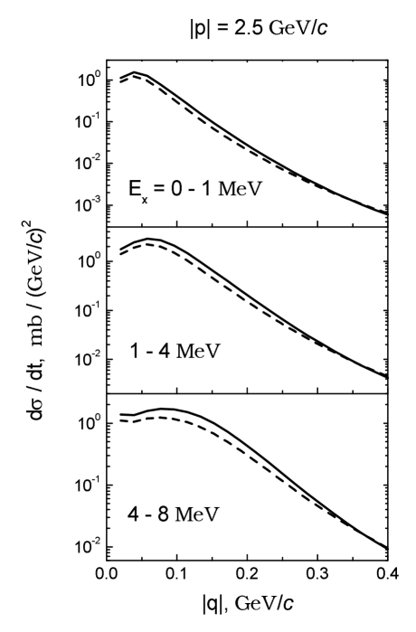
Figure 3: Unpolarized cross section, eq. (40), calculated within the relativistic impulse approximation at a typical COSY initial momentum for several bins of excitation energy of the $pp$ pair. Results of calculations with two parameterizations of the $NN$ charge-exchange amplitude are exhibited (solid curves are obtained with the amplitude from said ; saidpap , the dashed curves from diu ).

In Figs. 3 and 4 the cross section and tensor analyzing power $T_{20}$ for the process (1) are presented. The initial energy corresponds to a typical COSY momentum $|{\mbox{\bf p}}|=2.5$ GeV/c. The solid lines depict results with the elementary amplitude taken from ref. saidpap , whereas the dashed lines are results with the parameterization from ref. diu . As expected, since different parameterizations equally well reproduce the elementary charge-exchange cross section, the unpolarized cross section of the process (1) is not sensitive to parameterizations of the elementary amplitude. An opposite situation occurs when calculating the polarization observables defined in eq. (17) for which the contribution of partial amplitudes is non-diagonal and interferences might be important. This is clearly illustrated in Fig. 4, where the tensor analyzing power (18) exhibits indeed a strong sensitivity to parameterizations of partial amplitudes and practically does not depend upon the chosen bin of the excitation energy. From this picture one may conclude that an experimental investigation of the tensor analyzing power may constrain further parameterizations of the elementary charge-exchange amplitude at high energies.

As already mentioned, the process (1) has been experimentally investigated at SATURN-II kox . Although at such energies the final state interaction cannot be neglected and the simple impulse approximation is too rough, a comparison of data with theoretical results is rather instructive. In Figs. 5 and 6 we present results of calculations of the cross section (40) and tensor analyzing power $T_{20}$ (18) defined by eqs. (32-40) together with available experimental data. The full lines have been obtained with parameterizations of the elementary amplitude from refs. swart ; saidpap , while the dashed lines with the parameterization given in ref. diu . From Fig. 5 it is seen that the impulse approximation qualitatively describes the general shape of the cross section as a function of the transferred momentum $|{\mbox{\bf q}}|$. For low values of $|{\mbox{\bf q}}|$, say up to 0.2 GeV/c, and in the interval of the pair excitation energy $1\leq E_{x}\leq 4$ MeV here is even a good agreement with data, in contrast with other intervals of $E_{x}$ and higher values of $|{\mbox{\bf q}}|$. From this and from the results of non-relativistic calculations wil1 , where final state interaction and higher partial waves have been taken into account, one may conclude that at high values of transferred momentum the effects of final state interaction in the ${}^{1}S_{0}$ state become dominant. At higher excitation energies the interaction effects are not so significant, however here corrections from other partial waves may become important. The same conclusions can be drawn from Fig. 6, where the tensor analyzing power, computed with two parameterizations (as above, the solid lines correspond to ref. swart ; saidpap , dashed curves to ref. diu ), is compared with experimental data. From Fig. 6 it is also obvious that a qualitative agreement with data for the tensor analyzing power may be achieved only by using the elementary charge-exchange amplitude from the partial-wave analysis swart ; saidpap , while the parameterization diu results even in opposite sign for $T_{20}$. This is a direct indication that a more sophisticated partial-wave analysis gives more reliable partial helicity amplitudes. Nevertheless, since such an analysis has been performed for low and intermediate energies (up to few GeV), a further tuning of partial amplitudes (38) at relativistic energies is still desirable. Together with the proper choice of kinematics at high energies (i.e. a kinematical situation where the role of higher partial waves in the final state, e.g., triplet states, is suppressed glagolev ) one may expect that the proposed mechanism will adequately describe reactions of the type (1) and corresponding information may be obtained. Note that in all the above calculations the vector analyzing power is strictly zero.

V One-iteration approximation

As mentioned, for a consistent relativistic analysis of reactions with deuterons and two interacting nucleons in the continuum one should solve the BS equation for both bound state and scattering state within the same interaction kernel. We have found a numerical solution for the deuteron bound state with a realistic one-boson exchange potential solution . The BS equation, after a partial decomposition over a complete set of matrices in the spinor space, has been solved numerically by using an iteration method. We found that the iteration procedure converges rather quickly if the trial function is properly chosen, e.g., if in the BS equation the combination of the type (33) is used as trial functions with non-relativistic solutions of the Schrödinger equation. In such a case, even after the first iteration, the BS solution coincides with the exact one up to relative momentum $p\sim 0.6-0.7$ GeV/c. This circumstance can be used if one needs an approximate solution of the BS equation at not too large momenta $p\leq 0.5-0.7$ GeV/c. This is just our case, since in reaction (1) the relative momentum of the $pp$ pair is expected to be rather small and the scattering part of the amplitude (27) can be obtained from eq. (26) by one iteration, provided the trial function is properly chosen.

V.1 Formalities

To solve eq. (26) we proceed as follow (cf. ref. ourprc ): (i) for simplicity, in the inhomogeneous BS equation we leave only the pseudo-scalar isovector exchange ($\pi$-mesons), (ii) write instead of eq. (26) the mixed BS equation by introducing in both the left hand side and the free term the BS vertices, i.e.

$$G_{P}(p)=G^{0}_{P}(p)-ig^{2}_{\pi NN}\int\frac{d^{4}p^{\prime}}{(2\pi)^{4}}\frac{\gamma_{5}\Psi_{P}(p^{\prime})\gamma_{5}}{(p-p^{\prime})^{2}-\mu_{\pi}^{2}},$$ (44)

(iii) bearing in mind that the BS partial vertices may be obtained from the same spin-angular functions $\Gamma_{\alpha}({\bf p})$, by replacing ${\bf p}\leftrightarrow-{\bf p}$ quad , we write the corresponding partial BS equation

$$G_{{}^{1}\!S_{0}^{++}}(p_{0},|{\bf p}|) = G_{{}^{1}\!S_{0}^{++}}^{0}(p_{0},|{\bf p}|)$$ (45)

$$- ig^{2}_{\pi NN}\int\frac{d^{4}p^{\prime}d\Omega_{p}}{(2\pi)^{4}}\frac{(E_{p}E_{p^{\prime}}-m^{2}+({\bf p\,p}^{\prime}))}{E_{p}E_{p^{\prime}}}\frac{\phi_{1}(p_{0}^{\prime},|{\bf p}^{\prime}|)}{(p-p^{\prime})^{2}-\mu_{\pi}^{2}}.$$

Further by disregarding the dependence upon $p_{0}$ in the meson propagator in eq. (45) and then using the standard representation of propagators via generalized Legendre polynomials $Q_{l}$ and restoring the BS equation in terms of partial amplitudes, one obtains

$$\phi_{{}^{1}\!S_{0}^{++}}(p_{0},|{\mbox{\bf p}}|)=\phi_{{}^{1}\!S_{0}^{++}}^{0}(p_{0},|{\mbox{\bf p}}|)-\frac{g_{\pi NN}^{2}}{4\pi}\frac{1}{\left(\frac{1}{2}{\sqrt{s_{f}}}-E_{p}\right)^{2}-p_{0}^{2}}\times$$

$$\int\limits_{0}^{\infty}\frac{d|{\mbox{\bf p}}^{\prime}|}{2\pi}\,\frac{|{\mbox{\bf p}}^{\prime}|}{|{\mbox{\bf p}}|}\,\frac{1}{E_{p}E_{p^{\prime}}}\left[(E_{p}E_{p^{\prime}}-m^{2})Q_{0}({\tilde{y}}_{\mu})-|{\mbox{\bf p}}||{\mbox{\bf p}}^{\prime}|Q_{1}({\tilde{y}}_{\mu})\right]u_{{}^{1}\!S_{0}}(s_{f},|{\mbox{\bf p}}^{\prime}|),$$ (46)

where ${\tilde{y}}_{\mu}=\displaystyle\frac{{\mbox{\bf p}}^{2}+{\mbox{\bf p}}^{{}^{\prime}2}+\mu^{2}}{2|{\mbox{\bf p}}||{\mbox{\bf p}}^{\prime}|}$. In obtaining (46) the integration over $p_{0}^{\prime}$ has been carried out in the pole ${\tilde{p}}_{0}=\displaystyle\frac{1}{2}{\sqrt{s_{f}}}-E_{p^{\prime}}$ and, similar to eq. (33), we define the BS wave function in the continuum as

$$u_{{}^{1}\!S_{0}}(s_{f},|{\mbox{\bf p}}^{\prime}|)=\frac{g_{{}^{1}\!S_{0}^{++}}({\tilde{p}}_{0},|{\mbox{\bf p}}^{\prime}|)}{{\sqrt{s_{f}}}-2E_{p^{\prime}}}.$$ (47)

Now, if we restrict ourselves to only one iteration in (46) taking the trial function (47) as a non-relativistic solution of the Schrödinger equation, e.g. the Paris wave function $u^{NR}_{{}^{1}S_{0}}(s_{f},|{\mbox{\bf p}}^{\prime}|)$, the BS amplitude is obtained as

$$\phi_{{}^{1}\!S_{0}^{++}}(p_{0},|{\bf p}|)=\phi_{{}^{1}\!S_{0}^{++}}^{0}(p_{0},|{\bf p}|)-\frac{G^{o.i.}(\tilde{p}_{0},|{\bf p}|)}{\left(\frac{1}{2}{\sqrt{s_{f}}}-E_{p}\right)^{2}-p_{0}^{2}},$$ (48)

where the ”one-iteration” BS vertex $G^{o.i.}(\tilde{p}_{0},|{\bf p}|)$ is defined by

$$G^{o.i.}(\tilde{p}_{0},|{\bf p}|) = \frac{1}{\pi}\,\frac{g_{\pi NN}^{2}}{4\pi}\left\{\left[1-\frac{E_{p}}{m}\right]\int\limits_{0}^{\infty}dr\,e^{-\mu r}j_{0}(pr)\,u^{NR}_{{}^{1}\!S_{0}}(r)\right.$$ (49)

$$+ \left.\frac{|{\mbox{\bf p}}|}{mE_{p}}\int\limits_{0}^{\infty}dr\,\frac{u^{NR}_{{}^{1}\!S_{0}}(r)}{r}\,e^{-\mu r}\,(1-\mu r)\,j_{1}(pr)\right\}.$$

From eqs. (48) and (49) one can easily find the non-relativistic analogue of the obtained formulae. The free term in eq. (48) together with the first term in eq. (49) reflect the non-relativistic equation for the ${}^{1}S_{0}$ wave function, while the second term in (49) turns out to be a correction of purely relativistic origin.

V.2 Numerical results

In Figs. 7 and 8 we present results of numerical calculations of the cross section and tensor analyzing power $T_{20}$ given by eqs. (40), (18), (10), (25) and (48-49). The elementary charge-exchange amplitude has been taken from ref. saidpap and the non-relativistic trial function $u^{NR}_{{}^{1}S_{0}}(r)$ as the solution of the Schrödinger equation within the Paris potential paris_cont . The BS $S^{++}$ and $D^{++}$ amplitudes are those from the numerical solution solution obtained with a realistic one-boson exchange interaction. The dashed curves in Figs. 7 and 8 correspond to results within the relativistic impulse approximation, while the solid lines depict results with taking into account the final state interaction in one-iteration approximation. It is seen that in all three energy bins the agreement with data for the cross section is essentially improved. This concerns especially the range $1\leq E_{x}\leq 4$ MeV. For the energy bin close to zero there is still a disagreement with data at low transferred momenta which probably may be related to the fact that in our calculations we have not taken into account the Coulomb interaction within the $pp$ pair. For higher excitation energies ($E_{x}\sim 8$ MeV), other partial waves (e.g. triplet state) in the $pp$ final state contribute and, within the adopted assumptions, one may expect only semi-quantitative agreement with data. From Fig. 7 one may conclude that at low excitation energies the supposed mechanism for the reaction (1) (i.e. charge-exchange subprocess with interaction in ${}^{1}S_{0}$ state of the $pp$ pair in the continuum) seems to be correct. Moreover, from a comparison of the left and right panels in Fig. 7 one may expect that the higher initial energy the larger kinematical region where the mechanism holds. Fig. 8 demonstrates that the tensor analyzing power is less sensitive to final state interaction effects. As a matter of fact, the tensor analyzing power (18), being a ratio of non-diagonal products of partial amplitudes to the diagonal ones, serves as a measure of the quality of parameterization of partial amplitudes and their mutual relative phases. This has been pointed out in a series of publications (see e.g. refs. inclusive ; ourprc ), where a good simultaneous description of cross sections and $T_{20}$ in reactions of the deuteron break-up or elastic scattering of protons, is still lacking. Nevertheless, since in the process (1) the behavior of the partial amplitudes (16), as seen from eq. (25), is mostly governed by the elementary charge-exchange amplitudes, an experimental investigation of the tensor analyzing power $T_{20}$ in reactions of the type (1) can essentially supplement data on the $NN$ charge-exchange amplitudes at high energies.

In Figs. 9 and 10 we present the predicted cross section and tensor analyzing power at high energies relevant for COSY and Dubna accelerator. It is immediately seen that the cross section is substantially decreasing with increasing energy, nevertheless it remains large enough to be experimentally easily accessible. Another peculiarity of the studied process at relativistic energies is that the tensor analyzing power $T_{20}$ does not change the sign remaining positive in a large kinematical region, in contrast to lower energies (cf. Fig. 8). Note again, that in the above calculations the vector polarization of the deuteron is strictly zero.

From the performed analysis one can conclude that there is a kinematical region for the excitation energy, $E_{x}<5$ MeV, and transferred momentum, $|{\bf q}|\leq\,0.3-0.4$ GeV/c (i.e. the COSY cosy_proposal kinematics), for which the mechanism of the reaction (1) is fairly well described within the spectator approach by an elementary $pn$ charge-exchange subprocess, for active nucleons, with detection of the $pp$ pair in the ${}^{1}S_{0}$ final state. Our covariant approach agrees with previous non-relativistic calculations and allows for predictions of the cross sections and polarization observables at intermediate and relativistic energies, in particular, for kinematical conditions which are realized at COSY. The predicted cross sections of the process and the tensor analyzing power $T_{20}$ are large enough to be used, in a large range of initial energies, for determining properties of the polarized deuteron, provided experimentally one simultaneously detects a vanishing vector polarization of deuterons.

VI Summary

In summary, the performed covariant analysis of the reaction $\vec{D}(p,n)pp$ with the two final protons in a ${}^{1}S_{0}$ state allows us to conclude that, as in the non-relativistic limit, such a process can be used as an effective deuteron polarimeter also at relativistic energies, in particular, at the range covered by COSY at Jülich and upgraded Dubna accelerator. Additional information about the elementary charge-exchange amplitude at high energies can be obtained from precision data with known deuteron polarization.

VII Acknowledgments

We thank R. Arndt and I. Strakovsky for providing information about the use of their excellent SAID complex of programs. This work was performed in parts during the visits of S.S.S and L.P.K. in the Forschungszentrum Rossendorf, Institute of Nuclear and Hadron Physics. The support by the program ”Heisenberg-Landau” of JINR-FRG collaboration and the grants BMBF 06DR921, WTZ RUS 98/678 and RFBR 00-15-96737 are gratefully acknowledged.

Appendix A Deuteron state

The BS amplitudes of the deuteron, eq. (21), in the deuteron center of mass explicitly read

$$\Psi^{M}_{S^{++}}(k) = {\cal N}(\hat{k}_{1}+m)\frac{1+\gamma_{0}}{2}\hat{\xi}_{M}(\hat{k}_{2}-m)\psi_{S}(k_{0},|{\mbox{\bf k}}|),$$ (50)

$$\Psi^{M}_{D^{++}}(k) = -\frac{{\cal N}}{\sqrt{2}}(\hat{k}_{1}+m)\frac{1+\gamma_{0}}{2}$$ (51)

$$\times \left(\hat{\xi}_{M}+\frac{3}{2|{\mbox{\bf k}}|^{2}}(\hat{k}_{1}-\hat{k}_{2})(k\xi_{M})\right)(\hat{k}_{2}-m)\psi_{D}(k_{0},|{\mbox{\bf k}}|),$$

where $k_{1,2}$ are on-mass shell 4-vectors,

$$k_{1}=(E,{\mbox{\bf k}}),\quad k_{2}=(E,-{\mbox{\bf k}}),\quad k=(k_{0},{\mbox{\bf k}}),\quad E=\sqrt{{\mbox{\bf k}}^{2}+m^{2}},$$ (52)

and $\psi_{S,D}(k_{0},|{\mbox{\bf k}}|)$ are the partial scalar amplitudes, related to the corresponding partial vertices as

$$\psi_{S,D}(k_{0},|{\mbox{\bf k}}|)=\displaystyle\frac{G_{S,D}(k_{0},|{\mbox{\bf k}}|)}{\left(\displaystyle\frac{M_{D}}{2}-E\right)^{2}-k_{0}^{2}}.$$

In Eqs. (50-51) the normalization factor is ${\cal N}=\displaystyle\frac{1}{\sqrt{8\pi}}\displaystyle\frac{1}{2E(E+m)}$.

Appendix B ${}^{1}S_{0}$ state

Different representations of the BS amplitude ${}^{1}S_{0}$ in the continuum have been studied in details in ref. nashi , where the reader may found the most general expressions for the covariant amplitudes $b_{i}$, eq. (24), in terms of the partial amplitudes $\phi_{j}$ in the center of mass of the $pp$ pair. Since in the present paper we consider only the $++$ component of the $\phi_{i}$, we are left with one invariant function $b$, which is taken to be $b_{4}$. Then the explicit expressions for the kinematical coefficients $C_{1},C_{2},C_{3}$ in eq. (25) can be cast in the form

$$C_{1}=({\mbox{\bf p}}_{p}\cdot{\mbox{\bf k}})\,A_{1}-(E+m)\,(p_{p}^{0}+m)\,A_{2}-({\mbox{\bf q}}\cdot{\mbox{\bf p}}_{p})\,(E+m)\,A_{3}-({\mbox{\bf q}}\cdot{\mbox{\bf k}})\,(p_{p}^{0}+m)\,A_{4},$$

$$C_{2}=\frac{3}{\sqrt{2}(E-m)}\,[\,(E-m)\,A_{1}-(p_{p}^{0}+m)\,A_{2}-((2{\mbox{\bf k}}-{\mbox{\bf q}})\cdot{\mbox{\bf q}})\,A_{3}],$$

$$C_{3}=A_{1}-(E+m)\,A_{3}+(p_{p}^{0}+m)\,A_{4},$$

where

$$A_{1}={\cal K}\,[P_{0}^{\prime}\,(p_{p}^{0}+2m)+({\mbox{\bf q}}\cdot{\mbox{\bf p}}_{p})]-1,$$ (53)

$$A_{2}={\cal K}\,[P_{0}^{\prime}\,(p_{p}^{0}-2m)+({\mbox{\bf q}}\cdot{\mbox{\bf p}}_{p})]-1,$$ (54)

$$A_{3}=-{\cal K}\,(2m-p_{1}^{0}+p_{p}^{0}),$$ (55)

$$A_{4}=-{\cal K}\,(2m+p_{1}^{0}-p_{p}^{0}),$$ (56)

with the invariant coefficient ${\cal K}=\displaystyle\frac{1}{e\sqrt{s_{f}}}$ (see ref. nashi ). The 4-vectors $p_{1}$ and $p_{p}$ are defined by

$$p_{1}=\frac{1}{2}P^{\prime}+k-\frac{1}{2}q=(p_{1}^{0},{\mbox{\bf p}}_{p}),$$

$$p_{p}=(p_{p}^{0},{\mbox{\bf p}}_{p}),\quad p_{p}^{0}=\sqrt{m^{2}+{\mbox{\bf p}}_{p}^{2}},\quad{\mbox{\bf p}}_{p}={\mbox{\bf k}}-{\mbox{\bf q}}.$$

Observe, that $p_{p}$ represents an on-mass shell vector. Note also, that in the relativistic impulse approximation, since $p_{1}^{0}=p_{p}^{0}$, eqs. (53-56) are substantially simplified.

Appendix C Relativistic spin transformations

By definition, a state with given momentum p and helicity $\lambda$ in a frame of reference ${\cal O}$ is that obtained by a Lorenz transformation of a state with given spin projection $s_{z}$ from the rest system ${\cal O}_{rest}$ to ${\cal O}$, i.e.:

$$|{\mbox{\bf p}};\lambda\rangle\equiv|\stackrel{{\scriptstyle 0}}{{p}},s,s_{z}\rangle_{\cal O},$$ (57)

where $\stackrel{{\scriptstyle 0}}{{p}}=(m,0,0,0)$. As usual, a Lorenz transformation $h[{\mbox{\bf p}}]$ is presented by a sequence of two operations: a boost along the $z$ axis, $l_{z}(v)$, where $v$ is the speed of the state in ${\cal O}$, and a rotation from $z$ direction to the direction of p, i.e. ${\cal O}=r^{-1}(\phi,\theta,0)l_{z}^{-1}(v){\cal O}_{rest}$.

Let us suppose now that one has a state $|{\mbox{\bf p}};\lambda\rangle$ given in the frame ${\cal O}$ and one wishes to know how it reads in another frame ${\cal O}^{\prime}$ obtained by a Lorenz transformation $l$ on ${\cal O}$

$$|{\mbox{\bf p}};\lambda\rangle_{{\cal O}^{\prime}}=U(l^{-1})|{\mbox{\bf p}};\lambda\rangle.$$ (58)

From the definition of the helicity states one has

$$U(l^{-1})|{\mbox{\bf p}};\lambda\rangle=U(l^{-1})U(h[({\mbox{\bf p}})])|\stackrel{{\scriptstyle 0}}{{p}};\lambda\rangle,$$ (59)

where $h[{\mbox{\bf p}}]$ is the corresponding Lorenz transformation $\stackrel{{\scriptstyle 0}}{{p}}\to p$. Then multiplying eq. (59) by unity, $U(h[({\mbox{\bf p}}^{\prime})])U^{-1}[h[({\mbox{\bf p}}^{\prime})]=1$, where $h[{\mbox{\bf p}}^{\prime}]$ is the helicity transformation that defines a state $|{\mbox{\bf p}}^{\prime};\lambda\rangle=U(h[({\mbox{\bf p}}^{\prime}])|\stackrel{{\scriptstyle 0}}{{p}},\lambda\rangle$ with ${\mbox{\bf p}}^{\prime}$ being the same vector as obtained by transforming p from ${\cal O}$ to ${\cal O}^{\prime}$, one obtains:

$$U(l^{-1})|{\mbox{\bf p}};\lambda\rangle=U(h[({\mbox{\bf p}}^{\prime}]){\cal R}|\stackrel{{\scriptstyle 0}}{{p}},\lambda\rangle,$$ (60)

where ${\cal R}=U^{-1}[h[({\mbox{\bf p}}^{\prime})]U(l^{-1})U[h({\mbox{\bf p}})]$ is the sequence of transformations $\stackrel{{\scriptstyle 0}}{{p}}\to p\to p^{\prime}\to\stackrel{{\scriptstyle 0}}{{p}}$, i.e. nothing but a rotation. Then,

$$|{\mbox{\bf p}},\lambda\rangle_{{\cal O}^{\prime}}=D^{(s)}_{\lambda\lambda^{\prime}}(\omega)|{\mbox{\bf p}}^{\prime},\lambda^{\prime}\rangle,$$ (61)

where $\omega$ is a set of Euler angles describing the rotation. In case when the Lorenz transformation is a simple boost along the $z$ direction with the speed $\beta$, then $\omega$ is just an angle, describing a rotation about the $Y$ axis,

$$\cos\omega=\cos\theta^{\prime}\cos\theta+\gamma\sin\theta^{\prime}\sin\theta,$$ (62)

with $\gamma=1/\sqrt{1-\beta^{2}}$, and $\theta,\theta^{\prime}$ are the polar angles of p in the systems ${\cal O}$ and ${\cal O}^{\prime}$, respectively. This is known as Wick helicity rotation, contrary to Wigner’s canonical spin rotation. In our case, the relevant $z$ axis is the one along the direction of $({\mbox{\bf k}}+{\mbox{\bf p}})$. Then, obtaining the helicity amplitudes in the laboratory frame we need an additional rotation to change from the helicity basis to the spin projections.

Figure 1: Spectator mechanism for the charge-exchange process $pD\to n(pp)$. The Bethe-Salpeter amplitude for the deuteron bound state and the $pp$ pair in the continuum are denoted as $\Psi$ and $\bar{\Psi}$, respectively. The elementary $pn$ charge-exchange amplitude is symbolically represented by ${\cal A}^{ce}$.

Figure 2: Partial helicity amplitudes of eq. (38) vs. the transferred momentum $|{\bf q}|$ for different parameterizations. Solid curves correspond to the partial wave analysis of said ; saidpap , while the dashed curves are the high energy parameterization given in diu . The amplitudes are dimensionless.

Figure 4: The same as in Fig. 3 but for the tensor analyzing power $T_{20}$ (18).

Figure 5: Comparison of the non-polarized differential cross section eq. (40) within the impulse approximation at non-relativistic initial energies ($|{\mbox{\bf p}}|=0.444$ GeV/c (left panel) and $|{\mbox{\bf p}}|=0.599$ GeV/c (right panel)), with experimental data kox . Solid curves correspond to the elementary charge-exchange amplitude from the partial wave analysis from refs. said ; saidpap , dashed curves use diu .

Figure 6: The same as in Fig. 5 but for the tensor analyzing power $T_{20}$ (18).

Figure 7: Results of calculations of the differential cross section eq. (40) with taking into account the effects of final state interaction in ${}^{1}S_{0}$ state (solid curves). Experimental data are those from SATURN-II kox , the elementary amplitude has been taken from refs. said ; saidpap . The dashed curves depict the results of calculations within the pure impulse approximation (cf. solid curve in Fig. 5).

Figure 8: The same as in Fig. 7 but for the tensor analyzing power (18).

Figure 9: Results of calculations of the differential cross section (40) with taking into account the effects of final state interaction in ${}^{1}S_{0}$ state (solid curves). Kinematical conditions correspond to those proposed in cosy_proposal for experiments at COSY. Elementary amplitude from refs. said ; saidpap . The dashed curves depict results of calculations within the pure impulse approximation (cf. solid curves in Fig.3).

Figure 10: The same as in Fig. 9 but for the tensor analyzing power (18).

References

- (1) L.C. Alexa, et al., Phys. Rev. Lett. 82, 1374 (1999).
- (2) S. Kox, E.J. Beise (spokespersons), TJNAF experiment 94-018 ”Measurement of the Deuteron Polarization at Large Momentum Transvers in Scattering”; http://www.jlab.org/ex_prog; Phys. Rev. Lett. 84, 5053 (2000); Nucl. Phys. A 684, 521 (2001).
- (3) E. Tomasi-Gustafsson, in Proc. of XIV International Seminar On High Energy Physics Problems, Preprint JINR No. E1,2-2000-166 (Dubna, 2000).
- (4) V.I. Komarov (spokesman) et al., COSY proposal #20 updated from 1999, “Exclusive deuteron break-up study with polarized protons and deuterons at COSY”, http://ikpd15.ikp.kfa-juelich.de:8085/doc/Proposals.html.
- (5) R.G. Arnold, C.E. Carlson, F. Gross, Phys. Rev. C 23, 363 (1981).
-
(6)
M.P. Rekalo, I.M. Sitnik, Phys. Lett. B 356, 434 (1995);
L.S. Azhgirei et al., Phys. Lett. B 361, 21 (1995). -
(7)
V.G. Ableev et al., Nucl. Phys. A 393, 491 (1983);
C.F. Perdrisat, V. Punjabi, Phys. Rev. C 42, 1899 (1990);
B. Kühn, C.F. Perdrisat, E.A. Strokovsky, Phys. Lett. B 312, 298 (1994);
A.P. Kobushkin, A.I. Syamtomov, C.F. Perdrisat, V. Punjabi, Phys. Rev. C 50, 2627 (1994);
J. Erö et al., Phys. Rev. C 50, 2687 (1994);
J. Arvieux et al., Nucl. Phys. A 431, 6132 (1984). - (8) A.K. Kacharava et al., Preprint JINR No. E1-96-42 (Dubna, 1996); C.F. Perdrisat (spokesperson) et al., COSY proposal #68.1 ”Proton-to-proton polarization transfer in backward elastic scattering”.
-
(9)
M.P. Rekalo, N.M. Piskunov, I.M. Sitnik,
Few Body Syst. 23, 187 (1998);
Preprint JINR No. E4-96-328 (Dubna, 1996); Phys. At. Nucl. 57, 2089 (1994). -
(10)
V.P. Ladygin, N.B. Ladygina, J. Phys. G 23, 847 (1997);
V.P. Ladygin, Phys. At. Nucl. 60, 1238 (1997). - (11) L.P. Kaptari, B. Kämpfer, S.M. Dorkin, S.S. Semikh, Phys. Rev. C 57, 1097 (1998).
- (12) W. Grübler, P.A. Schmelzbach, V. König, Phys. Rev. C 22, 2243 (1980).
- (13) J. Yonnet et. al., in Proc. of XIII International Seminar On High Energy Physics Problems, Preprint JINR No. E1,2-98-154 (Dubna, 1998).
-
(14)
D.V. Bugg, C. Wilkin, Phys. Lett. B 152, 37 (1985);
D.V. Bugg, C. Wilkin, Nucl. Phys. A 467, 575 (1987). - (15) S. Kox et. al., Nucl. Instrum. Methods A 346, 527 (1994).
-
(16)
Y. Satou, S. Ishida, H. Sakai, H.Okamura, et al.,
Phys. Lett. B 521,
153 (2001);
Phys. Lett. B 314, 279 (1993);
H. Sakai, T. Wakasa, T. Nonaka, H. Okamura et al., Nucl. Phys. A 631, 757 (1998). - (17) T. Motobayashi et al., Phys. Lett. B 233, 69 (1989).
- (18) J. Carbonell, M. Barbaro, C. Wilkin, Nucl. Phys. A 529, 653 (1991).
- (19) S. Kox et. al., Nucl. Phys. A 556, 621 (1993).
-
(20)
D.V. Bugg, A. Hasan, R.L. Shypit, Nucl. Phys. A 477, 546 (1988);
C. Furget et. al., Nucl. Phys. A 631, 747 (1998). - (21) C.Mosbacher, F. Osterfeld, Phys.Rev. C 56 (1997) 2014.
- (22) M. Morlet et. al., Phys. Lett. B 247, 228 (1990).
- (23) B.S. Aladashvili et al., Nucl. Phys. B 86, 461 (1975).
- (24) H.H. Heckman et al., Phys. Lett. 35, 152 (1975).
- (25) L.P. Kaptari, A.I Titov, Sov. J. Nucl. Phys. 39, 612 (1984).
- (26) S.M. Dorkin, L.P. Kaptari, B. Kämpfer, S.S. Semikh, Phys. Atom. Nucl. 65 (2002) 442; Yad. Fiz. 65 (2002) 469.
-
(27)
A.Yu. Umnikov, L.P. Kaptari, F.C Khanna,
Phys. Rev. C 56, 1700 (1997);
A.Yu. Umnikov, L.P. Kaptari, K.Yu. Kazakov, F.C. Khanna, Phys. Lett. B 334, 163 (1994). - (28) A.Yu. Umnikov, Z. Phys. A 357, 333 (1997).
- (29) A. Bouquet, B. Diu, Nuovo Cimento 35A, 157 (1975).
- (30) P.W. Keaton, Jr., J.L. Gammel, G.G. Ohlsen, Ann. Phys. 85, 152 (1974).
- (31) F. Gross, Phys. Rev. 186, 1448 (1969).
- (32) C. Ciofi degli Atti, D. Farrali, A.Yu. Umnikov, L.P. Kaptari, Phys. Rev. C60, 034003 (1999).
- (33) S. Mandelstam, Proc. Roy. Soc. (London) A 233, 123 (1955).
- (34) S.G. Bondarenko, V.V. Burov, M. Beyer, S.M. Dorkin, Phys. Rev. C 58, 3143 (1998).
- (35) J.J. Kubis, Phys. Rev. D 6, 547 (1972).
- (36) L.P. Kaptari, A.Yu. Umnikov, S.G. Bondarenko, K.Yu. Kazakov, F.C. Khanna, B. Kämpfer, Phys. Rev. C 54, 986 (1996).
- (37) G.C. Wick, Phys. Rev. 96, 1124 (1954).
-
(38)
J. Fleischer, J. Tjon, Nucl. Phys. B 84, 375 (1975);
Phys. Rev. D 15, 2537 (1975)
M. Zuilhof, J. Tjon, Phys. Rev. C 22, 2369 (1980). - (39) V.M. Kolybasov, N.Ya. Smorodinskaya, Phys. Lett. B 37, 272 (1971).
- (40) L.P. Kaptari, B. Kämpfer, S.M. Dorkin, S.S. Semikh, Few - Body Systems 27, 189 (1999).
- (41) L.P. Kaptari, B. Kämpfer, S.M. Dorkin, S.S. Semikh, Phys. Lett. B 404, 8 (1997).
- (42) V.G.J. Stoks, R.A.M. Klomp, M.C.M. Rentmeester, J.J. de Swart, Phys. Rev. C 48, 792 (1993).
- (43) R.A. Arndt, I.I. Strakovsky, R.L. Workman, Phys.Rev. C 62 (2000) 034005.
- (44) http://nn-online.sci.kun.nl
- (45) http://gwdac.phys.gwu.edu
- (46) C. Bourrely, E. Leader, J. Soffer, Phys. Rep. 59, 95 (1980).
- (47) M. Lacombe, B. Loiseau, J.M. Richard, R. Vinh Mau et al., Phys. Rev. C 21, 861 (1980)