Magnetic dipole moment of the $\bm{S_{11}}$(1535) from the $\bm{\gamma p\to\gamma\eta p}$ reaction

Abstract

The $\gamma p\to\gamma\eta p$ reaction in the $S_{11}$(1535) resonance region is investigated as a method to access the $S_{11}$(1535) magnetic dipole moment. To study the feasibility, we perform calculations of the $\gamma p\to\gamma\eta p$ process within an effective Lagrangian approach containing both the $S_{11}$ resonant mechanism and a background of non-resonant contributions. Predictions are made for the forthcoming experiments. In particular, we focus on the sensitivity of cross sections and photon asymmetries to the $S_{11}$(1535) magnetic dipole moment.

1 Introduction

The study of the properties of the $S_{11}(1535)$ $N^{*}$ resonance, the lowest lying $J^{P}={\frac{1}{2}}^{-}$ nucleon resonance, provides valuable insight into the nature of QCD in the non-perturbative domain. In particular, the large mass splitting between the nucleon ground state $N(939)$ and its negative parity partner $N^{*}(1535)$ is connected to the spontaneous breaking of the chiral symmetry. Indeed, if the two-flavor chiral symmetry were exact and preserved by the QCD vacuum, QCD would predict parity doublets degenerate in mass [1, 2].

In recent years, new techniques have become available to perform numerical calculations of the properties of nucleon excited states using lattice QCD [3, 4, 5]. In particular, calculations of the mass spectrum of nucleon excited states were performed [3], which implement chiral symmetry at non-zero lattice spacing, by use of domain wall fermions. The recent quenched lattice QCD calculations [3, 4, 5], using different fermion actions, all reproduce quite well the observed large mass splitting between the nucleon and its negative parity partner $N^{*}(1535)$. Furthermore, the next generation of lattice QCD calculations opens up the exciting prospect to study how nucleon and resonance properties change when varying the quark mass parameter from the large quark mass regime, where chiral symmetry is explicitly broken, down to sufficiently small quark mass values, where one can use the chiral symmetry of QCD to perform the extrapolation to the chiral limit [6]. The large quark mass region may be the regime where a naive constituent quark picture could hold, and one may investigate how such a picture breaks down when approaching physical quark masses.

A particularly useful observable to study in this respect is the baryon magnetic dipole moment (MDM), as it has often been questioned and discussed [7, 8, 9] why the naive non-relativistic constituent quark model yields a relatively good agreement with the experimentally known values for the MDMs of the ground state octet baryons. Recently, it has been studied [10, 11] how the proton and neutron MDMs change when extrapolating from large up- and down-quark masses (about 6 - 10 times their physical mass values) where current lattice QCD calculations are performed, down to small quark masses, where the non-analytic behavior in the quark mass can be calculated from the chiral symmetry of QCD. In particular, it has been noticed in Ref. [11] that the apparent success of the non-relativistic constituent quark model in reproducing the observed ratio of proton to neutron MDMs at the physical quark masses is rather coincidental, supporting the finding of Ref. [7]. Therefore, it may be very revealing to extend such a study to the MDMs of nucleon resonances, such as the $\Delta(1232)$ and the $S_{11}(1535)$.

The $\Delta(1232)$ MDMs have been investigated on the lattice at rather large quark masses [12], and very recently the chiral extrapolation of the $\Delta(1232)$ MDMs, including the next-to-leading non-analytic variation with the quark mass, was also studied [13]. As there is a large gap in quark mass to bridge between the present quenched lattice QCD calculations and the chiral limit, it would be extremely helpful to know the resonance MDM for the physical quark mass values, through experiment. Unfortunately, the experimental information on the MDMs beyond the ground state baryon octet is very scarce. With the notable exception of the $\Omega^{-}$ baryon, these higher nucleon resonances decay strongly, and thus have too short lifetimes to measure their MDMs in the conventional way through spin precession measurements.

For the $\Delta^{++}(1232)$, it was therefore proposed to measure its MDM through the $\pi^{+}p\to\gamma\pi^{+}p$ reaction [14], and two experiments were performed [15, 16]. Using different theoretical analyses, the Particle Data Group (PDG) [17] quotes as range of the MDM : $\mu_{\Delta^{++}}=3.7-7.5\,\mu_{N}$, where $\mu_{N}$ is the nuclear magneton. The large uncertainty in the extraction of $\mu_{\Delta^{++}}$ from the data is due to large non-resonant contributions to the $\pi^{+}p\to\gamma\pi^{+}p$ reaction because of bremsstrahlung from the charged pion ($\pi^{+}$) and proton (p). Alternatively, it has been proposed [18] to determine the magnetic moment of the $\Delta^{+}(1232)$ through measurement of the $\gamma p\to\gamma\pi^{0}p$ reaction, thus avoiding bremsstrahlung contributions from the pions. First calculations for this reaction, including besides the $\Delta(1232)$ resonant mechanism [19, 20] also a background of non-resonant contributions, have recently been performed  [21, 22]. Due to the small cross sections of the $\gamma p\to\gamma\pi^{0}p$ reaction, the first experimental data have been obtained only very recently by the A2/TAPS Collaboration at the MAMI accelerator [23]. The pioneering experiment of Ref. [23] sees a clear deviation from the known soft bremsstrahlung processes (for which the final photon is radiated from the external proton lines), and the measured cross sections are in qualitatively good agreement with the calculation of Ref. [21]. The deviation from the soft bremsstrahlung contains a sensitivity to the magnetic dipole strength at the $\Delta(1232)$ resonance position. The experiment of Ref. [23] does not yet allow for a reliable extraction of this quantity, because of limited statistics. However, a dedicated experiment to measure the $\gamma p\to\gamma\pi^{0}p$ reaction is planned at MAMI in the near future [24]. This experiment will use the $4\pi$ Crystal Ball detector and thus increase the count rates by two orders of magnitude. In addition, this forthcoming experiment  [24] will be performed with a polarized photon beam, because the sensitivity of the $\gamma p\to\gamma\pi^{0}p$ reaction to the $\Delta^{+}(1232)$ MDM can be increased substantially when using linearly polarized photons, as has been shown in Ref. [21].

In the present paper, we explore the extension of this technique to access the MDM of the $S_{11}(1535)$ resonance. Since the $S_{11}(1535)$ resonance is known to dominate the $\gamma p\to\eta p$ reaction in the threshold region, the $\gamma p\to\gamma\eta p$ reaction, with a low energy outgoing photon (up to about 100 MeV), seems to be a promising tool to isolate the MDM of the $S_{11}(1535)$ resonance. Such an experiment can be envisaged using the Crystal Barrel@ELSA and in the near future with the Crystal Ball@MAMI, once the higher beam energy of about 1.5 GeV becomes available at MAMI-C.

In Section 2, we provide some model estimates for the $S_{11}(1535)$ MDM. In particular, we present the calculation of the $S_{11}(1535)$ MDM in the constituent quark model and contrast it with the value taken in the picture of the $S_{11}(1535)$ as a $(K\Sigma)$ quasi-bound (molecular) state, as has been proposed in Ref. [25].

We then develop in Section 3 an effective Lagrangian model for the $\gamma p\to\gamma\eta p$ reaction in the $S_{11}(1535)$ region, which is obtained by coupling a photon in a gauge invariant way to an analogous model for the $\gamma p\to\eta p$ reaction. The model contains both the $S_{11}(1535)$ resonance contribution and a background of non-resonant processes.

In Section 4, we discuss the model-independent link between the $\gamma p\to\eta p$ process and the $\gamma p\to\gamma\eta p$ process in the limit where the outgoing photon energy approaches zero. We present a low energy theorem, which provides a strong constraint for both the experiment and the theoretical description of the $\gamma p\to\gamma\eta p$ reaction.

In Section 5, we then use the developed effective Lagrangian model as a tool to study the feasibility of an experiment to measure the $\gamma p\to\gamma\eta p$ reaction. In particular, we investigate the sensitivity of the $\gamma p\to\gamma\eta p$ cross sections and photon asymmetries to the $S_{11}(1535)$ MDM. The final section summarizes our findings.

2 Model calculations for the $\bm{S_{11}(1535)}$ magnetic moment

In this section, we calculate the results for the MDM of the $S_{11}(1535)$ in the framework of the constituent quark model, and within the picture where the $S_{11}(1535)$ is dynamically generated as a $(K\Sigma)$ quasi-bound state, as first proposed in Ref. [25].

2.1 Magnetic moments in the constituent quark model

In the nonrelativistic SU(6) constituent quark model, the lowest-lying negative-parity nucleon resonances are $|N^{2}P_{1/2}\rangle$ and $|N^{4}P_{1/2}\rangle$, where the usual spectroscopic notations ${}^{2}P_{1/2}$ and ${}^{4}P_{1/2}$ are used to indicate their total quark spin $S=1/2,\,3/2$ ($2S+1=2,\,4$), orbital angular momentum $L=1$ ($P$-wave), and total angular momentum $J=1/2$. In contrast, the ground-state baryon octet (e.g., $N$, $\Lambda$, $\Sigma$) and decuplet (e.g., $\Delta$) have the same $S$-wave spatial wavefunctions with $L=0$, and thus $J=S$. The wavefunctions of the $|N^{2}P_{1/2}\rangle$ and $|N^{4}P_{1/2}\rangle$ states are given explicitly as

$$|N^{2}P_{1/2}\rangle=\frac{1}{\sqrt{2}}\sum_{m_{l}m_{s}}\langle\,1\,\tfrac{1}{2}\ m_{l}\,m_{s}\,|\,\tfrac{1}{2}\,\tfrac{1}{2}\,\rangle$$ (1)

$$\,\times\,\biggl{\{}\psi^{\rho}_{1m_{l}}\Bigl{[}\tfrac{1}{\sqrt{2}}\bigl{(}\chi^{\lambda}_{m_{s}}\,\phi^{\rho}+\chi^{\rho}_{m_{s}}\,\phi^{\lambda}\bigr{)}\Bigr{]}+\psi^{\lambda}_{1m_{l}}\Bigl{[}\tfrac{1}{\sqrt{2}}\bigl{(}\chi^{\rho}_{m_{s}}\,\phi^{\rho}-\chi^{\lambda}_{m_{s}}\,\phi^{\lambda}\bigr{)}\Bigr{]}\biggr{\}}\,,$$

$$|N^{4}P_{1/2}\rangle=\frac{1}{\sqrt{2}}\sum_{m_{l}m_{s}}\langle\,1\,\tfrac{3}{2}\,m_{l}\ m_{s}\,|\,\tfrac{1}{2}\,\tfrac{1}{2}\,\rangle\Bigl{[}\,\psi^{\rho}_{1m_{l}}\,\chi^{s}_{m_{s}}\,\phi^{\rho}+\,\psi^{\lambda}_{1m_{l}}\,\chi^{s}_{m_{s}}\,\phi^{\lambda}\,\Bigr{]}\,,$$ (2)

where $\psi$, $\chi$, and $\phi$ denote the spatial, spin, and flavor wavefunctions. The superscripts $s$ or $\rho$ ($\lambda$) of these wavefunctions indicate that they are totally symmetric among three quarks, or odd (even) under the exchange of the first two quarks. Further details can be found in Ref. [26].

However, the observed lowest-lying negative-parity nucleon resonances are the $S_{11}(1535)$ and $S_{11}(1650)$, obtained as configuration mixtures of the $|N^{2}P_{1/2}\rangle$ and $|N^{4}P_{1/2}\rangle$ SU(6) states,

$$|\,S_{11}(1535)\,\rangle = |\,N^{2}P_{1/2}\,\rangle\cos\vartheta-|\,N^{4}P_{1/2}\,\rangle\sin\vartheta\,,$$ (3)

$$|\,S_{11}(1650)\,\rangle = |\,N^{2}P_{1/2}\,\rangle\sin\vartheta+|\,N^{4}P_{1/2}\,\rangle\cos\vartheta\,,$$

where $\vartheta$ denotes the mixing angle.

In a constituent quark model, the magnetic dipole moments of $qqq$ baryons consist of contributions from both quark spin and orbital angular momentum, i.e. $\bm{\mu}=\bm{\mu^{S}}+\bm{\mu^{L}}$ with

$$\bm{\mu^{S}} = \sum_{i}\bm{\mu^{s}}_{i}=\sum_{i}\frac{Q_{i}}{m_{i}}\,\bm{s}_{i}\,,$$ (4)

$$\bm{\mu^{L}} = \sum_{i}\bm{\mu^{l}}_{i}=\sum_{i}\frac{Q_{i}}{2m_{i}}\,\bm{l}_{i}\,,$$ (5)

where the index $i$ sums over three quarks.

In Appendix A, we present the calculation of the spin and orbital contributions to the magnetic dipole moments for the states $|N^{2}P_{1/2}\rangle$ and $|N^{4}P_{1/2}\rangle$ with $J_{z}=+1/2$. The results are given by :

$$\mu(N^{2}P_{1/2}{}^{+}) = \langle\,N^{2}P_{1/2}{}^{+}\,|\,\mu_{z}\,|\,N^{2}P_{1/2}{}^{+}\,\rangle$$ (6)

$$= \tfrac{1}{9}\,(2\mu_{u}+\mu_{d})=\,\tfrac{1}{3}\;\mu_{N}\,,$$

$$\mu(N^{2}P_{1/2}{}^{\,0\,}) = \langle\,N^{2}P_{1/2}{}^{\,0\,}\,|\,\mu_{z}\,|\,N^{2}P_{1/2}{}^{\,0\,}\,\rangle$$ (7)

$$= \tfrac{1}{9}\,(2\mu_{d}+\mu_{u})=\ 0\,,$$

$$\mu(N^{4}P_{1/2}{}^{+}) = \langle\,N^{4}P_{1/2}{}^{+}\,|\,\mu_{z}\,|\,N^{4}P_{1/2}{}^{+}\,\rangle$$ (8)

$$= \tfrac{4}{9}\,(2\mu_{u}+\mu_{d})=\,\tfrac{5}{3}\;\mu_{N}\,,$$

$$\mu(N^{4}P_{1/2}{}^{\,0\,}) = \langle\,N^{4}P_{1/2}{}^{\,0\,}\,|\,\mu_{z}\,|\,N^{4}P_{1/2}{}^{\,0\,}\,\rangle$$ (9)

$$= \tfrac{4}{9}\,(2\mu_{d}+\mu_{u})=-\tfrac{1}{3}\;\mu_{N}\,,$$

where $\mu_{z}=\mu^{S}_{z}+\mu^{L}_{z}$, and the superscripts + and 0 denote the charge of the resonance state. Here we assume the constituent quarks as Dirac point particles and approximated $m_{u}=m_{d}=\tfrac{1}{3}\,m_{N}$. Using the relation $\mu=Q/2m$, we obtain $\mu_{u}=Q_{u}/2m_{u}=2\,\mu_{N}$ and $\mu_{d}=Q_{d}/2m_{d}=-\mu_{N}$, which are used to obtain the values in Eqs. (6)-(9).

In addition, there are the cross terms for $\mu^{S}_{z}$ which are obtained from mixing the $|N^{2}P_{1/2}\rangle$ and $|N^{4}P_{1/2}\rangle$ states,

$$\langle\,N^{4}P_{1/2}{}^{+}\,|\,\mu^{S}_{z}\,|\,N^{2}P_{1/2}{}^{+}\,\rangle=\langle\,N^{2}P_{1/2}{}^{+}\,|\,\mu^{S}_{z}\,|\,N^{4}P_{1/2}{}^{+}\,\rangle$$

$$= \tfrac{4}{9}\,(\mu_{u}-\mu_{d})=\tfrac{4}{\;3\;}\;\mu_{N}\,,$$

$$\langle\,N^{4}P_{1/2}{}^{\,0\,}\,|\,\mu^{S}_{z}\,|\,N^{2}P_{1/2}{}^{\,0\,}\,\rangle=\langle\,N^{2}P_{1/2}{}^{\,0\,}\,|\,\mu^{S}_{z}\,|\,N^{4}P_{1/2}{}^{\,0\,}\,\rangle$$

$$= \tfrac{4}{9}\,(\mu_{d}-\mu_{u})=-\tfrac{4}{3}\;\mu_{N}\,.$$ (11)

On the other hand, there are no cross terms for $\mu^{L}_{z}$ because $|N^{2}P_{1/2}\rangle$ and $|N^{4}P_{1/2}\rangle$ have orthogonal quark spin states which are not affected by $\mu^{L}_{z}$.

Now the magnetic moments of the $S_{11}(1535)$ and $S_{11}(1650)$ resonances can be expressed in terms of the magnetic moments of the $|N^{2}P_{1/2}\rangle$ and $|N^{4}P_{1/2}\rangle$ states and the cross terms,

$$\mu(S_{11}(1535)) = \mu(N^{2}P_{1/2})\cos^{2}\vartheta+\mu(N^{4}P_{1/2})\sin^{2}\vartheta$$

$$- 2\,\langle\,N^{2}P_{1/2}\,|\,\mu^{S}_{z}\,|\,N^{4}P_{1/2}\,\rangle\sin\vartheta\cos\vartheta\,,$$

$$\mu(S_{11}(1650)) = \mu(N^{2}P_{1/2})\sin^{2}\vartheta+\mu(N^{4}P_{1/2})\cos^{2}\vartheta$$

$$+ 2\,\langle\,N^{2}P_{1/2}\,|\,\mu^{S}_{z}\,|\,N^{4}P_{1/2}\,\rangle\sin\vartheta\cos\vartheta\,.$$

The value of the mixing angle $\vartheta$ depends on the quark interaction. Assuming a hyperfine interaction between the quarks, Isgur and Karl [26] predicted a mixing angle $\vartheta=\tan^{-1}{(\sqrt{5}-1)/2}\simeq-31.7^{\circ}$, which is close to the empirical mixing angle $\vartheta\simeq-32^{\circ}$ found in Ref. [27]. Using the value $\vartheta=-31.7^{\circ}$ in Eqs. (2.1) and (2.1), we obtain

$$\mu_{S_{11}^{+}(1535)} = 1.89\;\mu_{N}\quad\mathrm{and}\quad\mu_{S_{11}^{0}(1535)}=-1.28\;\mu_{N}\,,$$

$$\mu_{S_{11}^{+}(1650)} = 0.11\;\mu_{N}\quad\mathrm{and}\quad\mu_{S_{11}^{0}(1650)}=0.95\;\mu_{N}\,,$$

which agrees with the result by the Genova group [28]. Very similar results can also be obtained when the interactions of the $S_{11}$ resonances coupling to the $\pi N$ and $\eta N$ channels are explicitly considered [29].

2.2 Magnetic moment of $S_{11}(1535)$ as a $(K\Sigma)$ quasi-bound state

It has been proposed in Ref. [25] that the $S_{11}(1535)$ can be considered as a $(K\Sigma)$ quasi-bound state of mesons and baryons. Using an SU(3) effective chiral Lagrangian and iterating the derived coupled-channel potentials to infinite orders, the $S_{11}(1535)$ resonance can be generated dynamically. This finding has also been verified within the chiral unitary approach [31, 32]. Especially, in Ref. [32] it is found that the coupling of the $S_{11}(1535)$ to the $\eta N$ channel is nearly as large as the one to the $K\Sigma$ channel.

In a simplified picture, we regard the $S_{11}(1535)$ as a $(K\Sigma)$ quasi-bound state. Then the $S_{11}(1535)$ charge states can be written as :

$$|\,S^{+}_{11}(1535)\,\rangle \,=\, \sqrt{\frac{1}{3}}\,(K^{+}\,\Sigma^{0})\,+\,\sqrt{\frac{2}{3}}\,(K^{0}\,\Sigma^{+})\,,$$

$$|\,S^{0}_{11}(1535)\,\rangle \,=\, \sqrt{\frac{2}{3}}\,(K^{+}\,\Sigma^{-})\,-\,\sqrt{\frac{1}{3}}\,(K^{0}\,\Sigma^{0})\,.$$ (14)

From Eq. (14), it then follows that the magnetic moment of both $S_{11}(1535)$ charge states can be expressed in terms of the hyperon magnetic moments,

$$\mu_{S_{11}^{+}(1535)} \,=\, \frac{1}{3}\,\mu_{\Sigma^{0}}\,+\,\frac{2}{3}\,\mu_{\Sigma^{+}}\,,$$

$$\mu_{S_{11}^{0}(1535)} \,=\, \frac{2}{3}\,\mu_{\Sigma^{-}}\,+\,\frac{1}{3}\,\mu_{\Sigma^{0}}\,.$$ (15)

Using the experimental values for the $\Sigma^{+}$ and $\Sigma^{-}$ magnetic moments, and approximating the unknown $\Sigma^{0}$ magnetic moment by the average of the $\Sigma^{+}$ and $\Sigma^{-}$ magnetic moments, one obtains for the $S_{11}(1535)$ magnetic moments in the $(K\Sigma)$ molecule picture the values :

$$\mu_{S_{11}^{+}(1535)} \,=\, 1.86\;\mu_{N}\,,$$

$$\mu_{S_{11}^{0}(1535)} \,=\, -0.56\;\mu_{N}\,.$$ (16)

We like to stress that the calculation given here for the MDM of the $S_{11}(1535)$ as a $(K\Sigma)$ quasi-bound state is only a very simple exercise of the MDM for a dynamically generated resonance, and a full calculation within a coupled-channel framework remains to be done. In this respect, the magnetic moment of the $\Lambda(1405)$, which is in the same lowest energy $J^{P}={\frac{1}{2}}^{-}$ baryon octet as the $S_{11}(1535)$, has recently been evaluated in Ref. [33] using unitarized chiral perturbation theory. In this approach the $\Lambda(1405)$ is dynamically generated. It would be very worthwhile to also perform such a calculation for the MDM of the $S_{11}(1535)$ resonance.

3 Effective Lagrangian model

In this section we develop an effective Lagrangian model for the $\gamma p\to\gamma\eta p$ reaction in the $S_{11}(1535)$ resonance region, which will subsequently be used as a tool to investigate the sensitivity to the $S_{11}(1535)$ MDM.

In the $\gamma p\to\gamma\eta p$ process, a photon ($k$, $\lambda$) hits a proton target ($p_{N}$, $s_{N}$); in the final state, a photon ($k^{\prime}$, $\lambda^{\prime}$), an $\eta$ meson ($q$), and a proton ($p^{\prime}_{N}$, $s^{\prime}_{N}$) are observed. Here $k$, $k^{\prime}$, $p_{N}$, $p^{\prime}_{N}$, and $q$ are the four-momentum for the respective particles, $\lambda$ and $\lambda^{\prime}$ denote the photon helicity, and $s_{N}$ and $s^{\prime}_{N}$ are the proton spin projection.

For convenience, our results for the experimental observables will be expressed in the center-of-mass (c.m.) frame of the initial $\gamma p$ system. The kinematics of the $\gamma p\to\gamma\eta p$ reaction can be described by five variables. First, we choose the energies $E_{\gamma}^{\mathrm{cm}}$ and $E^{\prime\mathrm{cm}}_{\gamma}$ of the initial and outgoing photon, respectively. The other three variables are the polar and azimuthal angles $\theta_{\gamma}^{\mathrm{cm}}$, $\phi_{\gamma}^{\mathrm{cm}}$ of the final photon, and $\theta_{\eta}^{\mathrm{cm}}$ the polar angle of the eta meson. They are defined by choosing the plane which contains the initial particles and the final $\eta$ to be the $xz-$plane with $\bm{k}$ pointing in the $z$-direction, and thus $\phi_{\eta}^{\mathrm{cm}}\equiv 0$.

The unpolarized five-fold differential cross section for the $\gamma p\to\gamma\eta p$ reaction, which is differential with respect to the outgoing photon energy and angles as well as the eta meson angles in the c.m. system, is given by

$$\frac{d\sigma}{dE^{\prime\mathrm{cm}}_{\gamma}\,d\Omega_{\gamma}^{\mathrm{cm}}\,d\Omega_{\eta}^{\mathrm{cm}}}\; = \;\frac{1}{(2\pi)^{5}}\,{\frac{1}{32\sqrt{s}}}\,\frac{E^{\prime\mathrm{cm}}_{\gamma}}{E^{\mathrm{cm}}_{\gamma}}\,\frac{|\,\bm{q}\,|^{2}}{|\,\bm{q}\,|(E^{\prime}_{p}+\omega_{q})+E^{\prime\mathrm{cm}}\omega_{q}\cos\theta_{\gamma^{\prime}\eta}}\,$$ (17)

$$\times \left(\,\frac{1}{4}\sum_{\lambda}\sum_{s_{N}}\sum_{\lambda^{\prime}}\sum_{s_{N}^{\prime}}|\,\varepsilon_{\mu}(k,\lambda)\,\varepsilon_{\nu}^{*}(k^{\prime},\lambda^{\prime})\,{\mathcal{M}}^{\nu\mu}\,|^{2}\,\right)\,,$$

where $\omega_{q}$ and $\bm{q}$ are the energy and momentum of the eta meson, $E^{\prime}_{p}$ is the final proton energy, $\theta_{\gamma^{\prime}\eta}$ the c.m. angle between the outgoing photon and the eta, and $\varepsilon_{\mu}(k,\lambda)$ and $\varepsilon_{\nu}^{*}(k^{\prime},\lambda^{\prime})$ are the polarization vectors of the incoming and outgoing photons, respectively. Furthermore, ${\mathcal{M}}^{\nu\mu}$ is a tensor for the $\gamma p\to\gamma\eta p$ process, which will be calculated next within an effective Lagrangian model.

To develop a model for the $\gamma p\to\gamma\eta p$ reaction, we start from an effective Lagrangian model for the $\eta$ photoproduction reaction $\gamma p\to\eta p$, whose parameters are determined by a fit to the experimental data. The fixed parameters are subsequently used to calculate the $\gamma p\to\gamma\eta p$ process. The dominant contributions for $\eta$ photoproduction in the $S_{11}(1535)$ region are shown in Fig. 1. These include, in addition to the resonance contribution, the nucleon Born terms and the $t$-channel vector meson exchanges as the nonresonant background. Besides the dominant $S_{11}(1535)$ nucleon resonance, we also include the $S_{11}(1650)$ since its contribution in the $S_{11}(1535)$ region is not negligible. Other nucleon resonances are neglected at this stage since their contributions to the $\eta$ photoproduction cross sections in the $S_{11}(1535)$ region are small.

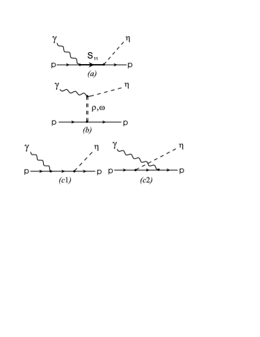
Figure 1: Diagrams for the $\gamma p\rightarrow\eta p$ reaction in the $S_{11}(1535)$ region : $S_{11}$ resonance excitation (a), vector meson exchange (b), and Born diagrams (c1,c2).

To extend our description to the $\gamma p\rightarrow\gamma\eta p$ reaction, we couple a photon in a gauge invariant way to all charged particles in Fig. 1. The resulting diagrams are shown in Fig. 2, where the $\gamma$-$S_{11}$-$S_{11}$ vertex in diagram (a2) contains contribution from the magnetic moments of the $S_{11}$ resonances. Here we assume that the anomalous MDM of the ${S_{11}^{+}(1650)}$ vanishes, because it has only a very small effect in the $S_{11}(1535)$ region and its predicted value from the quark model is small (see Sec. 2.1). Therefore, in comparison with the $\gamma p\to\eta p$ process, the only new parameter entering in the description of the $\gamma p\rightarrow\gamma\eta p$ process is the $S_{11}^{+}(1535)$ anomalous magnetic moment $\kappa_{S_{11}^{+}(1535)}$. In the following, we discuss the $S_{11}$ resonance as well as the background contributions to the $\gamma p\rightarrow\gamma\eta p$ reaction.

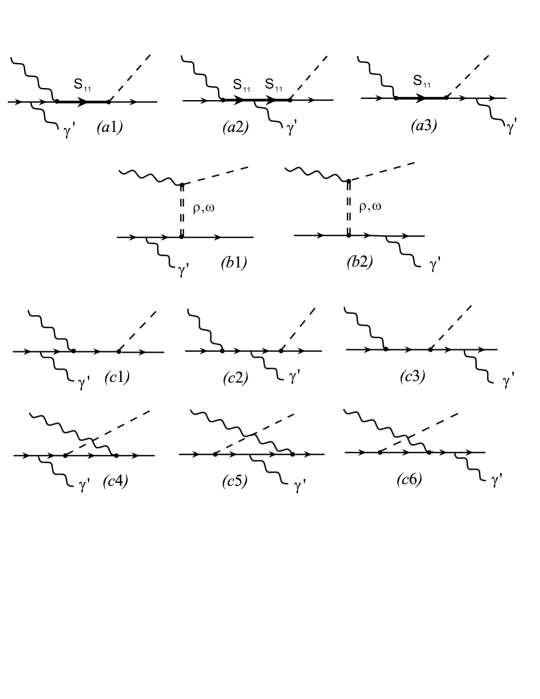
Figure 2: Diagrams considered in the calculation of the $\gamma p\rightarrow\gamma\eta p$ reaction in the $S_{11}(1535)$ region, obtained by gauge invariant coupling of a photon to the diagrams of Fig. 1 : $S_{11}$ resonance diagrams (a1-a3), vector-meson exchange diagrams (b1-b2), and Born diagrams (c1-c6).

3.1 $S_{11}(1535)$ resonance propagator

As the $S_{11}(1535)$ resonance is a spin-1/2 particle, its Feynman propagator is given by :

$$G_{R}(p)=\frac{1}{p/-M_{R}}\,,$$ (18)

where $p$ is the four-momentum and $M_{R}$ the mass of the $S_{11}$(1535). To take account of the finite width of the $S_{11}$ resonance, we follow the procedure of Refs. [34, 35] by using a complex pole description for the resonance excitation. This amounts to the replacement

$$M_{R}\,\longrightarrow\,M_{R}-\frac{i}{2}\,\Gamma_{R}\,$$ (19)

in the propagator of Eq. (18). This ‘complex mass scheme’ guarantees electromagnetic gauge invariance. In contrast, the use of a Breit-Wigner propagator with an energy-dependent width will violate gauge invariance when applied to the $S_{11}$ contribution for the $\gamma p\rightarrow\gamma\eta p$ reaction. By fitting the $\gamma p\rightarrow\eta p$ data in the $S_{11}(1535)$ region, we can determine the complex pole of the $S_{11}(1535)$. The fit results are shown in Fig. 3. Limiting our fit to the data near the $S_{11}(1535)$ peak in the range $E_{\gamma}^{\mathrm{lab}}=730-880$ MeV, we obtain $(M_{R},~{}\Gamma_{R})$ = (1490, 154) MeV, which will be used in our calculation for the $\gamma p\rightarrow\gamma\eta p$ process. In comparison, the value given by the PDG [17] is (1505, 170) MeV. However, using the PDG value the agreement with the photoproduction data is less satisfactory.

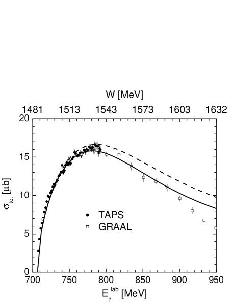
Figure 3: Total cross section for the $\gamma p\rightarrow\eta p$. The solid line is the full result, and the dashed line indicates the contribution from the $S_{11}(1535)$. The data are from TAPS [36] and GRAAL [37].

3.2 $S_{11}(1535)$ resonance amplitudes

The interaction Lagrangians relevant for the resonance contribution ($R=S_{11}$) in the $\gamma p\rightarrow\gamma\eta p$ process are

$$\mathcal{L}_{\gamma RR} = -e\,\bar{\psi}_{R}\left[\,e_{R}\gamma_{\mu}A^{\mu}-\tfrac{\kappa_{R}}{2M_{R}}\sigma_{\mu\nu}\partial^{\nu}A^{\mu}\right]\psi_{R}\,,$$

$$\mathcal{L}_{\gamma NR} = -\tfrac{e}{2(M_{N}+M_{R})}\,\bar{\psi}_{R}\,\kappa_{NR}\,\gamma_{5}\,\sigma_{\mu\nu}\,\psi_{N}F^{\mu\nu}+\mathrm{h.c.}\,,$$

$$\mathcal{L}_{\eta NR} = -\,i\,g_{\eta NR}\,\bar{\psi}_{N}\,\psi_{R}\,\phi_{\eta}+\mathrm{h.c.}\,,$$ (20)

where $g_{\eta NR}$ is the pseudoscalar coupling for the $\eta NR$ vertex, $e_{R}$ and $\kappa_{R}$ the resonance charge and the anomalous magnetic dipole moment, $\kappa_{NR}$ the $N\rightarrow R$ transition magnetic coupling, and $F^{\mu\nu}=\partial^{\mu}A^{\nu}-\partial^{\nu}A^{\mu}$.

Using these effective Lagrangians, we can derive the amplitudes for the $S_{11}$ resonance contributions in Fig. 1(a) and Fig. 2(a1-a3). The amplitude for the $S_{11}$(1535) resonance contribution to the $\gamma p\to\eta p$ process, corresponding to Fig. 1(a), is given by

$$\varepsilon_{\mu}(k,\lambda)\,{\mathcal{M}}^{\mu}_{a}(\gamma p\to\eta p)\,$$ (21)

$$= \,i\,\tfrac{e\,g_{\eta NR}}{M_{N}+M_{R}}\,\varepsilon_{\mu}(k,\lambda)\,k_{\alpha}\bar{N}(p^{\prime}_{N},s^{\prime}_{N})\,G_{R}(p_{R})\,\kappa_{pR}\,\gamma_{5}\,\sigma^{\mu\alpha}\,N(p_{N},s_{N})\,,$$

where $G_{R}$ is the $S_{11}$ propagator given by Eqs. (18) and (19).

Starting from Eq. (21) to the $\gamma p\to\eta p$ process, we now construct the corresponding $S_{11}$ contribution to the $\gamma p\to\gamma\eta p$ process. This is obtained by coupling a photon in a gauge invariant way to all charged particles in Fig. 1(a). First we obtain the diagrams with a photon attached to an external proton [Figs. 2(a1) and 2(a3)], described by the usual Dirac and Pauli currents with $\kappa_{p}=1.79$ for the proton anomalous MDM. The contributions of these diagrams to the tensor ${\mathcal{M}}^{\nu\mu}$ of Eq. (17) are given by

$${\mathcal{M}}^{\nu\mu}_{a1}(\gamma p\to\gamma\eta p)$$ (23)

$$= \,i\,\tfrac{e^{2}g_{\eta NR}}{M_{N}+M_{R}}\,k_{\alpha}\,\bar{N}(p^{\prime}_{N},s^{\prime}_{N})\,G_{R}(p^{\prime}_{R})\,\kappa_{pR}\,\gamma_{5}\,\sigma^{\mu\alpha}$$

$$\times\;S_{N}(p_{N}-k^{\prime})\left[\gamma^{\nu}-\kappa_{p}\,i\sigma^{\nu\beta}\tfrac{k^{\prime}_{\beta}}{2M_{N}}\right]N(p_{N},s_{N})\,,$$

$${\mathcal{M}}^{\nu\mu}_{a3}(\gamma p\to\gamma\eta p)$$

$$= \,i\,\tfrac{e^{2}g_{\eta NR}}{M_{N}+M_{R}}\,k_{\alpha}\,\bar{N}(p^{\prime}_{N},s^{\prime}_{N})\left[\gamma^{\nu}-\kappa_{p}\,i\sigma^{\nu\beta}\tfrac{k^{\prime}_{\beta}}{2M_{N}}\right]$$

$$\times\;S_{N}(p^{\prime}_{N}+k^{\prime})\,G_{R}(p_{R})\,\kappa_{pR}\,\gamma_{5}\,\sigma^{\mu\alpha}\,N(p_{N},s_{N})\,,$$

where $p^{\prime}_{R}$ and $p_{R}$ correspond to the four-momenta of the $S_{11}$ resonance in Fig. 2(a1) and 2(a3). In the soft-photon limit ($k^{\prime}\to 0$), the coupling of the photon to the external lines gives the only contribution. However, at finite energy for the emitted photon, gauge invariance also requires the diagram with a photon attached to the intermediate $S_{11}$ resonance [Fig. 2(a2)], which corresponds to the tensor,

$${\mathcal{M}}^{\nu\mu}_{a2}(\gamma p\to\gamma\eta p)$$ (24)

$$= \,i\,\tfrac{e^{2}g_{\eta NR}}{M_{N}+M_{R}}\,k_{\alpha}\,\bar{N}(p^{\prime}_{N},s^{\prime}_{N})\,G_{R}(p^{\prime}_{R})\,\Gamma_{\gamma RR}^{\,\nu}\,G_{R}(p_{R})$$

$$\times\;\kappa_{pR}\,\gamma_{5}\,\sigma^{\mu\alpha}\,N(p_{N},s_{N})\,,$$

with $G_{R}(p_{R})$ and $G_{R}(p^{\prime}_{R})$ the $S_{11}$ propagators before and after emitting the photon in Fig. 2(a2), and the $\gamma RR$ vertex

$$\Gamma_{\gamma RR}^{\,\nu}\,=\,\gamma^{\nu}\,-\,i\,\kappa_{R}\,\sigma^{\nu\beta}\,\tfrac{k^{\prime}_{\beta}}{2M_{R}}\,,$$ (25)

containing the photon coupling to the charge of a spin 1/2 field of a Dirac particle [34] as well as the $S_{11}$ Pauli current proportional to $\kappa_{R}$.

The vertex for a point spin-1/2 particle follows from the requirement of gauge invariance. Indeed, only the sum of the three diagrams (a1, a2, a3) in Fig. 2 is gauge-invariant, which is expressed through the electromagnetic Ward identity relating the $\gamma RR$ vertex with the $S_{11}$ propagator,

$$\left(p^{\prime}_{R}-p_{R}\right)_{\nu}\,G(p^{\prime}_{R})\;\Gamma_{\gamma RR}^{\,\nu}\;G(p_{R})\,=\,G(p_{R})\,-\,G(p^{\prime}_{R})\,.$$ (26)

To include the finite width of the $S_{11}$, the ‘complex mass scheme’ was advocated in Ref. [34], i.e., the replacement of $M_{R}$ by the complex mass of Eq. (19). In doing so, it is easily checked that the Ward identity of Eq. (26) still holds. On the other hand, when using Breit-Wigner propagators, and replacing $M_{R}^{2}$ in the denominator of Eq. (18) by $M_{R}^{2}\,-\,i\,M_{R}\,\Gamma_{R}(W)$, with $\Gamma_{R}(W)$ an energy dependent width, one immediately sees that the ${S_{11}}$ propagators before and after the emission of the photon have different widths (except for the soft-photon limit $k^{\prime}\to 0$, where the contribution of diagram Fig. 2(a2) vanishes relative to those of Fig. 2(a1) and (a3)). Therefore, when using energy-dependent widths at finite energy of the emitted photon, it is not possible to maintain the Ward identity of Eq. (26) with the vertex of Eq. (25).

3.3 Background contributions

The effective Lagrangians relevant to the background contribution in the $\gamma p\rightarrow\gamma\eta p$ process are

$$\mathcal{L}_{\gamma NN} = -e\,\bar{\psi}_{N}\left[\,\hat{e}_{N}\gamma_{\mu}A^{\mu}-\tfrac{\kappa_{N}}{2M_{N}}\sigma_{\mu\nu}\partial^{\nu}A^{\mu}\right]\psi_{N}\,,$$

$$\mathcal{L}_{\eta NN} = -i\,g_{\eta NN}\,\bar{\psi}_{N}\,\gamma_{5}\,\psi_{N}\,\phi_{\eta}\,,$$

$${\mathcal{L}}_{\gamma\eta V} = \tfrac{e\lambda_{\gamma\eta V}}{m_{\eta}}\,\varepsilon_{\mu\nu\rho\sigma}\,(\partial^{\mu}A^{\nu})\,\phi_{\eta}\,(\partial^{\rho}V^{\sigma})\,,$$

$${\mathcal{L}}_{VNN} = g_{VNN}{\bar{\psi}_{N}}\left(\gamma_{\mu}V^{\mu}+\tfrac{\kappa_{V}}{2m_{N}}\sigma_{\mu\nu}\partial^{\nu}V^{\mu}\right)\,\psi_{N}\,,$$ (27)

where $V$ denotes $\rho$ and $\omega$ vector meson fields, and the pseudoscalar coupling $g_{\eta NN}$ is used in our calculation. With these effective Lagrangians, it is straightforward to derive the amplitudes corresponding to the diagrams of Fig. 1(b) and (c1,c2) as well as Fig. 2(b1,b2) and (c1-c6).

For the $\eta NN$ coupling in Eq. (27), we determine its value by fitting the photoproduction data and obtain $g_{\eta NN}^{2}/4\pi=0.05$. For the vector meson couplings, we use the values from Ref. [38]. There are uncertainties associated with the $g_{\eta NN}$ and vector meson couplings, and it could affect the correct extraction of the $S_{11}(1535)$ MDM. However, the background contributions, which contain the Born terms and vector meson exchanges, do not exceed $1\%$ of the $\gamma p\to\eta p$ and $\gamma p\to\gamma\eta p$ cross sections in the $S_{11}(1535)$ energy region considered here. Therefore, we believe that these uncertainties will not significantly affect the extraction of the $S_{11}(1535)$ MDM.

4 Soft photon limit

In the soft photon limit ($k^{\prime}\rightarrow 0$), gauge invariance provides a model-independent relation between the cross sections for the $\gamma p\rightarrow\gamma\eta p$ and $\gamma p\rightarrow\eta p$ processes. In this section, we formulate this low energy theorem. The expression we derive applies to the production of any neutral meson $M$, and we therefore refer more generally to the $\gamma p\rightarrow\gamma Mp$ reaction in this section. In particular, it also applies to the $\gamma p\rightarrow\gamma\pi^{0}p$ reaction as studied in Ref. [21].

All variables in this section are expressed in the c.m. frame of the initial $\gamma p$ system. In the soft photon limit, the momentum and energy of the outgoing photon vanishes, and the $\gamma p\rightarrow\gamma Mp$ reaction is dominated by the bremsstrahlung process from the initial and final protons. In this limit, when integrating the five-fold differential cross sections for the $\gamma p\rightarrow\gamma Mp$ process over the outgoing photon angles, we obtain (the details are given in Appendix B)

$$\frac{d\sigma}{dE^{\prime\mathrm{cm}}_{\gamma}d\Omega^{\mathrm{cm}}_{M}}\longrightarrow\frac{1}{E^{\prime\mathrm{cm}}_{\gamma}}\frac{e^{2}}{2\pi^{2}}\,W(v)\left(\frac{d\sigma}{d\Omega_{M}}\right)^{\!\mathrm{cm}}\quad\mathrm{as}\ k^{\prime}\rightarrow 0\,.$$ (28)

Here $(d\sigma/d\Omega_{M})^{\!\mathrm{cm}}$ is the differential cross section for the $\gamma p\rightarrow Mp$ process, and we define an angular weight-function

$$W(v)\equiv-1+\left(\frac{v^{2}+1}{2v}\right)\ln\left(\frac{v+1}{v-1}\right)\,,$$ (29)

where $v\equiv\sqrt{1+\frac{4M_{N}^{2}}{-t}}$ with $t=(k-q)^{2}$ and $M_{N}$ the nucleon mass.

If we integrate the cross section of Eq. (28) also over the meson angles, the result is

$$\frac{d\sigma}{dE^{\prime\mathrm{cm}}_{\gamma}} \equiv \int d\Omega^{\mathrm{cm}}_{M}\frac{d\sigma}{dE^{\prime\mathrm{cm}}_{\gamma}d\Omega^{\mathrm{cm}}_{M}}\,,$$

$$\longrightarrow \frac{1}{E^{\prime\mathrm{cm}}_{\gamma}}\cdot\bar{\sigma}_{M}\quad\mathrm{as}\ k^{\prime}\rightarrow 0\,,$$

with a “weight-averaged” total cross section,

$$\bar{\sigma}_{M}\equiv\frac{e^{2}}{2\pi^{2}}\int d\Omega^{\mathrm{cm}}_{M}\,W(v)\left(\frac{d\sigma}{d\Omega_{M}}\right)^{\!\mathrm{cm}}\,.$$ (31)

Figure 4: Angular weight-function $W(v)$ of Eq. (29) in the soft-photon formula for the $\gamma p\rightarrow\gamma\eta p$ (solid curve) and $\gamma p\rightarrow\gamma\pi^{0}p$ (dashed curve) processes, as function of the meson angle $\theta_{M}^{cm}$.

We show the angular weight-function $W(v)$ in Fig. 4 for both the $\gamma p\rightarrow\gamma\eta p$ and the $\gamma p\rightarrow\gamma\pi^{0}p$ processes. If the meson is emitted in the forward direction with respect to the initial photon direction, there appears a destructive interference between the bremsstrahlung from the initial and final nucleons, whereas for a meson emitted in the backward direction both bremsstrahlung sub-processes add constructively.

The low energy theorem of Eq. (4) provides a check for both theoretical model calculations and experimental measurements, because the ratio

$$R\,\equiv\,E^{\prime\mathrm{cm}}_{\gamma}\cdot(d\sigma/dE^{\prime\mathrm{cm}}_{\gamma})/\bar{\sigma}_{M},$$ (32)

with $d\sigma/dE^{\prime\mathrm{cm}}_{\gamma}$ for $\gamma p\rightarrow\gamma Mp$ and $\bar{\sigma}_{M}$ for $\gamma p\rightarrow Mp$, approaches unity when $k^{\prime}\rightarrow 0$.

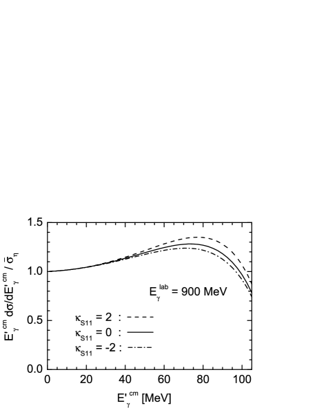
Figure 5: Outgoing photon energy dependence of the ratio $R$, defined in Eq. (32), for the $\gamma p\rightarrow\gamma\eta p$ reaction at $E_{\gamma}^{\mathrm{lab}}=900$ MeV.

In Fig. 5, we show the ratio $R$ constructed from our theoretical calculations of the $\gamma p\rightarrow\gamma\eta p$ and $\gamma p\rightarrow\eta p$ reactions. We indeed observe that $R$ approaches unity when $k^{\prime}\rightarrow 0$. For $k^{\prime}\simeq 20$ MeV, this ratio is still within 5% of the soft photon limit. Upon increasing the outgoing photon energy further, one starts to see clear deviations (of the order of 30%) from the soft photon limit. These deviations allow one to extract new resonance information from the $\gamma p\rightarrow\gamma\eta p$ reaction, which will be studied in the next section.

5 Results for $\bm{\gamma\,p\to\gamma\,\eta\,p}$ observables

In this section, we use our effective Lagrangian model as a tool to study the feasibility of an experiment to measure the $\gamma p\to\gamma\eta p$ reaction. In particular, we present our results for the $\gamma p\to\gamma\eta p$ cross sections and photon asymmetries for different values of $\kappa_{S_{11}(1535)}$ in the range of the estimates made in Section 2, i.e., between $-2$ to $+2$ (in units of $\mu_{N}$), to illustrate the sensitivity with respect to the $S_{11}(1535)$ MDM.

Figure 6: Outgoing photon energy dependence of the cross section $d\sigma/dE^{\prime\mathrm{cm}}_{\gamma}$ (integrated over photon and eta angles) for the $\gamma p\rightarrow\gamma\eta p$ reaction at $E_{\gamma}^{\mathrm{lab}}=900$ MeV.

In Fig. 6, we show the outgoing photon energy dependence of the cross section $d\sigma/dE^{\prime\mathrm{cm}}_{\gamma}$ for the $\gamma p\rightarrow\gamma\eta p$ reaction integrated over the photon and eta angles for fixed $E_{\gamma}^{\mathrm{lab}}=900$ MeV. The cross section at low energies $E^{\prime\mathrm{cm}}_{\gamma}$ exhibits the characteristic bremsstrahlung behavior, but displays clear deviations from such a behavior when going to higher outgoing photon energies (see also Fig. 5). To give an idea about the feasibility to measure the $\gamma p\rightarrow\gamma\eta p$ cross section, it is worthwhile to make the comparison with the $\gamma p\to\gamma\pi^{0}p$ reaction in the $\Delta(1232)$ region, which has already been measured [23]. At zero outgoing photon energy, the cross section for radiative eta production can be estimated from the $\gamma p\rightarrow\eta p$ cross section. On the other hand, the maximum value of the $\gamma p\rightarrow\eta p$ cross section at the $S_{11}(1535)$ position is about 5 % of the $\gamma p\rightarrow\pi^{0}p$ cross section at the $\Delta(1232)$ position. However, at an outgoing photon energy of about 100 MeV, which is the region where it is sensitive to the MDM of the resonance, our estimate for the $\gamma p\to\gamma\eta p$ reaction at $E_{\gamma}^{\mathrm{lab}}=900$ MeV yields count rates that are about 10–15 % of the measured value of Ref. [23] in case of the $\gamma p\to\gamma\pi^{0}p$ reaction at $E_{\gamma}^{\mathrm{lab}}=450$ MeV, which turns out to be much more favorable than the 5 % found in the soft photon limit.

Figure 7: Outgoing photon energy dependence of the $E^{\prime\mathrm{cm}}\cdot d^{3}\sigma/dE^{\prime\mathrm{cm}}_{\gamma}d\Omega^{\mathrm{cm}}_{\eta}$ for the $\gamma p\rightarrow\gamma\eta p$ reaction at $E_{\gamma}^{\mathrm{lab}}=900$ MeV.

One can increase the sensitivity of the $\gamma p\rightarrow\gamma\eta p$ reaction to the $S_{11}(1535)$ MDM by measuring differential cross sections in specific kinematical regions. In Fig. 7, we show the cross section, in the c.m. frame of the initial $\gamma p$ system, for different values of the $\eta$ angle upon integration over all photon directions at $E_{\gamma}^{\mathrm{lab}}=900$ MeV. At the lower energies, one sees a strong forward-backward asymmetry, which was discussed before in Fig. 4, yielding substantially larger cross sections for backward $\eta$ c.m. angles. However, at $E^{\prime\mathrm{cm}}_{\gamma}\approx 100$ MeV, the cross sections become comparable for all angles and exhibit a 20% change when $\kappa_{S_{11}(1535)}$ is varied between $-2$ to $+2$.

Figure 8: Outgoing photon energy dependence of $E^{\prime\mathrm{cm}}\cdot d^{5}\sigma/dE^{\prime\mathrm{cm}}_{\gamma}d\Omega^{\mathrm{cm}}_{\gamma}d\Omega_{\eta}^{\mathrm{cm}}$ and photon asymmetry $\Sigma$ of the $\gamma p\rightarrow\gamma\eta p$ reaction for fixed polar angles $\theta_{\eta}^{\mathrm{cm}}=90^{\circ}$ and $\theta_{\gamma}^{\mathrm{cm}}=45^{\circ}$, and varying azimuthal angle $\phi_{\gamma}^{\mathrm{cm}}=0^{\circ},\;90^{\circ},\;180^{\circ}$ (from left to right) at $E_{\gamma}^{\mathrm{lab}}=900$ MeV.

One can further increase the sensitivity by measuring cross sections at particular angular regions of the emitted $\eta$ and $\gamma$. As an example, we show in Fig. 8 the five-fold c.m. differential cross section $d^{5}\sigma/dE^{\prime\mathrm{cm}}_{\gamma}d\Omega_{\gamma}^{\mathrm{cm}}d\Omega_{\eta}^{\mathrm{cm}}$ and the photon asymmetry $\Sigma$ at $E_{\gamma}^{\mathrm{lab}}=900$ MeV for the polar angles $\theta_{\eta}^{\mathrm{cm}}=90^{\circ}$ and $\theta_{\gamma}^{\mathrm{cm}}=45^{\circ}$, and for three values of the azimuthal angle $\phi_{\gamma}^{\mathrm{cm}}=0^{\circ},\;90^{\circ},\ {\rm{and}}\ 180^{\circ}$ (note that the $\eta$ is emitted in the plane, i.e., $\phi_{\eta}^{\mathrm{cm}}\equiv 0^{\circ}$). We notice that the photon asymmetries reach values of about 10% around $E^{\prime\mathrm{cm}}_{\gamma}=100$ MeV, and show a strong dependence on the out-of-plane angle of the emitted photon. One also finds that the sensitivity of the photon asymmetry to the value of $\kappa_{S_{11}(1535)}$ is quite sizeable.

6 Summary and conclusions

In this paper we investigated the $\gamma p\to\gamma\eta p$ reaction in the $S_{11}$(1535) resonance region as a tool to access the $S_{11}$(1535) magnetic dipole moment (MDM). We performed calculations of the $\gamma p\to\gamma\eta p$ process using an effective Lagrangian approach, which contains the $S_{11}(1535)$ and $S_{11}(1650)$ resonant mechanism as well as a background of non-resonant contributions. As a starting point, the effective Lagrangian formalism is first applied to the $\gamma p\to\eta p$ reaction. When extending the calculation to the $\gamma p\to\gamma\eta p$ process, a photon is coupled to all charged particles in the $\gamma p\to\eta p$ process, and the coupling is constrained by gauge invariance. In particular, to take account of the finite width of the $S_{11}$ resonance, a complex mass scheme rather than a Breit-Wigner propagator with energy-dependent widths, has been used to maintain the Ward identity.

We presented our results for the $\gamma p\to\gamma\eta p$ process using both unpolarized and polarized photon beams. In particular, we focused on the sensitivity of cross sections and photon asymmetries to the $S_{11}$(1535) anomalous MDM. We derived a low–energy theorem relating the cross sections for the $\gamma p\to\eta p$ and $\gamma p\to\gamma\eta p$ processes in the soft-photon limit, which provides a useful check for both theoretical calculations and experimental measurements.

We first showed the unpolarized cross section integrated over the full photon and $\eta$ angles. At low energies this cross section is dominated by the bremsstrahlung contribution, which is consistent with our check in the soft-photon limit. The sensitivity of the unpolarized integrated cross section to $\kappa_{S_{11}(1535)}$ is found to be small, but can be increased by measuring differential cross sections at particular angular ranges. For the differential cross section $d^{3}\sigma/dE^{\prime\mathrm{cm}}_{\gamma}d\Omega_{\eta}^{\mathrm{cm}}$ integrated over the photon angles (but not the $\eta$ angles), and the five-fold differential cross section $d^{5}\sigma/dE^{\prime\mathrm{cm}}_{\gamma}d\Omega^{\mathrm{cm}}_{\gamma}d\Omega_{\eta}^{\mathrm{cm}}$, we found that the change when varying $\kappa_{S_{11}(1535)}$ between $-2$ to $+2$ is at the 20%–25% level. One can further increase the sensitivity by measuring cross sections using a linearly polarized photon beam. Indeed, our results clearly show that the sensitivity of the photon asymmetry to $\kappa_{S_{11}(1535)}$ is quite sizeable.

One inspiring motivation to study the MDMs of the $S_{11}(1535)$ resonance is to clarify the nature of this resonance—whether it is a traditional $qqq$ state, or dynamically generated from meson-baryon interactions. In the framework of the SU(6) quark model, the $S_{11}(1535)$ and $S_{11}(1650)$ resonances are configuration mixtures of two SU(6) states with excited orbital wavefunctions. Calculating both the quark spin and orbital angular momentum contribution for the MDM, as well as the cross terms due to the configuration mixing, we obtained the MDM values for the $S_{11}(1535)$ resonance. In comparison, we also presented a simple MDM calculation, where the $S_{11}$(1535) is dynamically generated and described as a ($K\Sigma$) molecule. Of course, further predictions of $S_{11}(1535)$ MDMs from other baryon resonance calculations would be most welcome, since through this reaction we can investigate the MDMs of orbitally excited nucleon resonances for the first time by an experiment. Although challenging, such investigations seem now feasible at ELSA and MAMI. These planned experiments will provide an interesting test for every baryon structure calculation, and give insight into the nature of the parity partner of the nucleon.

Appendix A Quark model calculation

To perform a calculation in a constituent quark model with harmonic wave functions, it is convenient to work with Jacobi coordinates, which are defined in terms of the three quark positions $\bm{r_{i}}$,

$$\bm{R} = \tfrac{1}{\;3\;}\,(\bm{r_{1}}+\bm{r_{2}}+\bm{r_{3}})\,,$$ (33)

$$\bm{\rho} = \tfrac{1}{\sqrt{2}}\,(\bm{r_{1}}-\bm{r_{2}})\,,$$

$$\bm{\lambda} = \tfrac{1}{\sqrt{6}}\,(\bm{r_{1}}+\bm{r_{2}}-2\bm{r_{3}})\,.$$

Their inversion relations are

$$\bm{r_{1}} = \bm{R}+\tfrac{1}{\sqrt{2}}\,\bm{\rho}+\tfrac{1}{\sqrt{6}}\,\bm{\lambda}\,,$$ (34)

$$\bm{r_{2}} = \bm{R}-\tfrac{1}{\sqrt{2}}\,\bm{\rho}+\tfrac{1}{\sqrt{6}}\,\bm{\lambda}\,,$$

$$\bm{r_{3}} = \bm{R}-\sqrt{\tfrac{2}{3}}\,\bm{\lambda}\,.$$

We usually calculate in the center-of-mass system of the three quarks in a baryon, i.e., $\bm{R}\equiv 0$.

In a constituent quark model, the MDM of a baryon consists of contributions from both quark spin and orbital angular momentum,

$$\bm{\mu} = \bm{\mu^{S}}+\bm{\mu^{L}}\,,$$ (35)

$$\bm{\mu^{S}} = \sum_{i}\bm{\mu^{s}}_{i}=\sum_{i}\frac{Q_{i}}{m_{i}}\,\bm{s}_{i}\,,$$ (36)

$$\bm{\mu^{L}} = \sum_{i}\bm{\mu^{l}}_{i}=\sum_{i}\frac{Q_{i}}{2m_{i}}\,\bm{l}_{i}\,,$$

$$= \sum_{i}\frac{Q_{i}}{2m_{i}}\,\bm{r}_{i}\times{\bm{p}}_{i}\,,$$

$$= \frac{Q_{1}+Q_{2}}{4m}\,\bm{l_{\rho}}+\Bigl{(}\frac{Q_{1}+Q_{2}}{12m}+\frac{Q_{3}}{3m^{\prime}}\Bigr{)}\,\bm{l_{\lambda}}+\frac{Q_{1}-Q_{2}}{4\sqrt{3}m}\,\bigl{(}\bm{\rho}\times{\bm{p_{\lambda}}}+\bm{\lambda}\times{\bm{p_{\rho}}}\bigr{)}\,,$$

where $Q_{i}$ denotes the charge of the $i$th quark, the index $i$ sums over three quarks, and $\bm{l_{\rho}}=\bm{\rho}\times{\bm{p_{\rho}}}$, $\bm{l_{\lambda}}=\bm{\lambda}\times{\bm{p_{\lambda}}}$.

The calculation for the quark spin part of baryon MDMs is straightforward. But the calculation for the orbital angular momentum part is much less familiar, since it vanishes for ground state octet and decuplet baryons, which have no orbital excitation. To calculate the matrix elements of $\mu^{L}_{z}$ with wavefunctions of Eq. (1), we need to operate on spatial wavefunctions $\psi^{\rho,\lambda}_{1m}$ with $z$-components of $\bm{l_{\lambda}}$, $\bm{l_{\rho}}$, $\bm{\rho}\times{\bm{p_{\lambda}}}$, and $\bm{\lambda}\times{\bm{p_{\rho}}}$. We list in the following the properties where $\mu^{L}_{z}$ acts on spatial wavefunctions $\psi_{1m}$,

$$\left.\begin{array}[]{rclcrcl}l_{\rho z}\,\psi^{\rho}_{1m}&=&m\,\psi^{\rho}_{1m}\,,&&l_{\rho z}\,\psi^{\lambda}_{1m}&=&0\,,\\[4.30554pt] l_{\lambda z}\,\psi^{\lambda}_{1m}&=&m\,\psi^{\lambda}_{1m}\,,&&l_{\lambda z}\,\psi^{\rho}_{1m}&=&0\,,\\[4.30554pt] (\bm{\rho}\times\bm{p_{\lambda}})_{z}\,\psi^{\lambda}_{1m}&=&m\,\psi^{\rho}_{1m}\,,&&(\bm{\rho}\times\bm{p_{\lambda}})_{z}\,\psi^{\rho}_{1m}&=&0\,,\\[4.30554pt] (\bm{\lambda}\times\bm{p_{\rho}})_{z}\,\psi^{\rho}_{1m}&=&m\,\psi^{\lambda}_{1m}\,,&&(\bm{\lambda}\times\bm{p_{\rho}})_{z}\,\psi^{\lambda}_{1m}&=&0\,.\end{array}\right.$$ (38)

In the case of a symmetric $qqq$ state $|\,(qqq)_{s}\,\rangle$, the calculation of $\bm{\mu^{L}}$ can be simplified as

$$\langle\,(qqq)_{s}\,|\,\bm{\mu^{L}}\,|\,(qqq)_{s}\,\rangle=\langle\,(qqq)_{s}\,|\,\frac{Q_{3}}{m_{3}}\,\bm{l_{\lambda}}\,|\,(qqq)_{s}\,\rangle\,.$$ (39)

In the Tables 1-4, we list the matrix elements for quark spin and orbital angular momentum contributions of the MDMs for the states $|\,N^{2}P_{1/2}\,\rangle$ and $|\,N^{4}P_{1/2}\,\rangle$ with $J_{z}=+1/2$.

Table 1: Matrix elements for $\langle\,N^{2S+1}P_{1/2}{}^{+}\,|\,\mu^{S}_{z}\,|\,N^{2S+1}P_{1/2}{}^{+}\,\rangle$

$\mu^{S}_{z}$	$|\,N^{2}P_{1/2}{}^{+}\,\rangle$	$|\,N^{4}P_{1/2}{}^{+}\,\rangle$
$\langle\,N^{2}P_{1/2}{}^{+}\,|$	$-\frac{1}{9}\,(2\mu_{u}+\mu_{d})$	$\frac{4}{9}\,(\mu_{u}-\mu_{d})$
$\langle\,N^{4}P_{1/2}{}^{+}\,|$	$\frac{4}{9}\,(\mu_{u}-\mu_{d})$	$\frac{5}{9}\,(2\mu_{u}+\mu_{d})$

Table 2: Matrix elements for $\langle\,N^{2S+1}P_{1/2}{}^{0}\,|\,\mu^{S}_{z}\,|\,N^{2S+1}P_{1/2}{}^{0}\,\rangle$

$\mu^{S}_{z}$	$|\,N^{2}P_{1/2}{}^{0}\,\rangle$	$|\,N^{4}P_{1/2}{}^{0}\,\rangle$
$\langle\,N^{2}P_{1/2}{}^{+}\,|$	$-\frac{1}{9}\,(2\mu_{d}+\mu_{u})$	$\frac{4}{9}\,(\mu_{d}-\mu_{u})$
$\langle\,N^{4}P_{1/2}{}^{+}\,|$	$\frac{4}{9}\,(\mu_{d}-\mu_{u})$	$\frac{5}{9}\,(2\mu_{d}+\mu_{u})$

Table 3: Matrix elements for $\langle\,N^{2S+1}P_{1/2}{}^{+}\,|\,\mu^{L}_{z}\,|\,N^{2S+1}P_{1/2}{}^{+}\,\rangle$

$\mu^{L}_{z}$	$|\,N^{2}P_{1/2}{}^{+}\,\rangle$	$|\,N^{4}P_{1/2}{}^{+}\,\rangle$
$\langle\,N^{2}P_{1/2}{}^{+}\,|$	$\tfrac{1}{9}\bigl{(}2\tfrac{Q_{u}}{m_{u}}+\tfrac{Q_{d}}{m_{d}}\bigr{)}$	0
$\langle\,N^{4}P_{1/2}{}^{+}\,|$	0	$-\tfrac{1}{18}\bigl{(}\tfrac{Q_{u}}{m_{u}}+2\tfrac{Q_{d}}{m_{d}}\bigr{)}$

Table 4: Matrix elements for $\langle\,N^{2S+1}P_{1/2}{}^{0}\,|\,\mu^{L}_{z}\,|\,N^{2S+1}P_{1/2}{}^{0}\,\rangle$

$\mu^{L}_{z}$	$|\,N^{2}P_{1/2}{}^{0}\,\rangle$	$|\,N^{4}P_{1/2}{}^{0}\,\rangle$
$\langle\,N^{2}P_{1/2}{}^{0}\,|$	$\tfrac{1}{9}\bigl{(}2\tfrac{Q_{d}}{m_{d}}+\tfrac{Q_{u}}{m_{u}}\bigr{)}$	0
$\langle\,N^{4}P_{1/2}{}^{0}\,|$	0	$-\tfrac{1}{18}\bigl{(}\tfrac{Q_{d}}{m_{d}}+2\tfrac{Q_{u}}{m_{u}}\bigr{)}$

Appendix B Derivation of the low energy theorem relating the $\bm{\gamma p\to\gamma Mp}$ and $\bm{\gamma p\to Mp}$ processes

In the limit $k^{\prime}\to 0$, the $\gamma p\rightarrow\gamma Mp$ reaction is exactly described by the bremsstrahlung process from the initial and final protons. This yields the five-fold differential c.m. cross section

$$\frac{d\sigma}{dE^{\prime\mathrm{cm}}_{\gamma}d\Omega^{\mathrm{cm}}_{M}d\Omega^{\mathrm{cm}}_{\gamma}}$$

$$\longrightarrow \left(\frac{d\sigma}{d\Omega_{M}}\right)^{\!\mathrm{cm}}\,\cdot\,\frac{e^{2}}{16\pi^{3}}\,E^{\prime\mathrm{cm}}_{\gamma}\,\cdot\,\sum_{\lambda_{\gamma}}\left|\,\frac{p^{\prime}_{N}\cdot\varepsilon(k^{\prime},\lambda_{\gamma})}{p^{\prime}_{N}\cdot k^{\prime}}\;-\;\frac{p_{N}\cdot\varepsilon(k^{\prime},\lambda_{\gamma})}{p_{N}\cdot k^{\prime}}\,\right|^{2},$$

as $k^{\prime}\rightarrow 0$. In Eq. (B), $(d\sigma/d\Omega_{M})^{\mathrm{cm}}$ is the c.m. cross section for the $\gamma p\rightarrow Mp$ process, $\lambda_{\gamma}=\pm 1$ is the soft photon polarization, and $\varepsilon$ its polarization vector. We calculate the RHS of Eq. (B), by performing the sum over the photon polarizations, and integrating over the photon angles. This gives the result :

$$\frac{d\sigma}{dE^{\prime\mathrm{cm}}_{\gamma}d\Omega^{\mathrm{cm}}_{M}}\longrightarrow\left(\frac{d\sigma}{d\Omega_{M}}\right)^{\!\mathrm{cm}}\,\cdot\,\frac{e^{2}}{16\pi^{3}}\,E^{\prime\mathrm{cm}}_{\gamma}\,\cdot\;I\,,$$ (41)

where we introduced the photon angular integral $I$ as :

$$I\,\equiv\,\int d\Omega^{\mathrm{cm}}_{\gamma}\,\left[\,\frac{2\,p_{N}\cdot p^{\prime}_{N}}{(p_{N}\cdot k^{\prime})\,(p^{\prime}_{N}\cdot k^{\prime})}\,-\,\frac{M^{2}}{(p_{N}\cdot k^{\prime})^{2}}\,-\,\frac{M^{2}}{(p^{\prime}_{N}\cdot k^{\prime})^{2}}\,\right].$$ (42)

In Eq. (42), the second and third terms arise from the contribution of bremsstrahlung from the same proton, whereas the first term stems from the interference between the bremsstrahlung from the initial and final protons.

We next work out the photon angular integral of Eq. (42). It turns out to be useful to introduce the initial and final nucleon velocities $\bm{\beta_{N}}\equiv\bm{p_{N}}/E_{N}$ and $\bm{\beta^{\prime}_{N}}\equiv\bm{p^{\prime}_{N}}/E^{\prime}_{N}$, and a Feynman parametrization in the first term of Eq. (42), which brings the two propagator factors to the same denominator. This leads to the expression :

$$I\,= \,\frac{2\pi}{(E^{\prime\mathrm{cm}}_{\gamma})^{2}}\cdot\left\{(1-\bm{\beta_{N}}\cdot\bm{\beta^{\prime}_{N}})\,\int_{-1}^{+1}dy\,\int_{-1}^{+1}dx\,\frac{1}{(1-\beta_{y}\,x)^{2}}\right.$$

$$\ \left.\,-\,(1-\beta_{N}^{2})\int_{-1}^{+1}dx\,\frac{1}{(1-\beta_{N}\,x)^{2}}\,-\,(1-\beta^{\prime 2}_{N})\int_{-1}^{+1}dx\,\frac{1}{(1-\beta^{\prime}_{N}\,x)^{2}}\right\},$$

where $\beta_{N}$, $\beta^{\prime}_{N}$, and $\beta_{y}$ are the magnitudes of $\bm{\beta_{N}}$, $\bm{\beta^{\prime}_{N}}$, and $\bm{\beta_{y}}$, which are related by

$$\bm{\beta_{y}}\,\equiv\,\bm{\beta_{N}}\,\frac{1}{2}(1+y)\;+\;\bm{\beta^{\prime}_{N}}\,\frac{1}{2}(1-y)\,.$$ (44)

The $x$-integrals in Eq. (B) can be worked out using

$$\int_{-1}^{+1}dx\,\frac{1}{(1-\beta\,x)^{2}}\,=\,\frac{2}{1-\beta^{2}}\,,$$ (45)

which yields for Eq. (B) the result :

$$I\,=\,\frac{2\pi}{(E^{\prime\mathrm{cm}}_{\gamma})^{2}}\,\cdot\left\{-4\,+\,2\,(1-\bm{\beta_{N}}\cdot\bm{\beta^{\prime}_{N}})\,\int_{-1}^{+1}dy\,\frac{1}{(1-\beta_{y}^{2})}\right\}.$$ (46)

By defining the variable $v\equiv\sqrt{1+\frac{4M_{N}^{2}}{-t}}$, with $t=(k-p_{M})^{2}=(p^{\prime}_{N}-p_{N})^{2}$, we express

$$(1-\bm{\beta_{N}}\cdot\bm{\beta^{\prime}_{N}})\,=\,(1-\beta_{N}^{2})^{1/2}\,\cdot\,(1-{\beta^{\prime}_{N}}^{2})^{1/2}\,\cdot\,\left(\frac{v^{2}+1}{v^{2}-1}\right),$$ (47)

and after a little algebra we can work out the remaining integral using :

$$\int_{-1}^{+1}dy\,\frac{1}{(1-\beta_{y}^{2})}\,=\,\frac{1}{(1-\beta_{N}^{2})^{1/2}\,\cdot\,(1-\beta^{\prime 2}_{N})^{1/2}}\,\cdot\,\left(\frac{v^{2}-1}{2v}\right)\,2\,\ln\left(\frac{v+1}{v-1}\right).$$ (48)

Combining Eqs. (46-48), we obtain the result for the photon angular integral $I$,

$$I\,=\,\frac{2\pi}{(E^{\prime\mathrm{cm}}_{\gamma})^{2}}\,\cdot 4\cdot\left\{-1\,+\,\left(\frac{v^{2}+1}{2v}\right)\,\ln\left(\frac{v+1}{v-1}\right)\right\}.$$ (49)

Using Eq. (49), the soft photon limit for the cross section of Eq. (41) then leads to the result of Eq. (28).

References

- [1] C. DeTar and T. Kunihiro, Phys. Rev. D 39 (1989) 2805.
- [2] D. Jido, M. Oka and A. Hosaka, Prog. Theor. Phys. 106 (2001) 873.
- [3] S. Sasaki, T. Blum and S. Ohta, Phys. Rev. D 65 (2002) 074503.
- [4] M. Göckeler et al., Phys. Lett. B 532 (2002) 63.
- [5] W. Melnitchouk et al., hep-lat/0202022.
- [6] A.W. Thomas, in Proceedings of the 20th International Symposium On Lattice Field Theory (LATTICE 2002), to be published in Nucl. Phys. B, Proceedings Supplement; hep-lat/0208023.
- [7] G. Morpurgo, Phys. Rev. D 46 (1992) 4068.
- [8] T.P. Cheng and L.-F. Li, Phys. Rev. Lett. 80 (1998) 2789.
- [9] G. Dillon and G. Morpurgo, hep-ph/0211256.
- [10] D.B. Leinweber, D.H. Lu and A.W. Thomas, Phys. Rev. D 60 (1999) 034014.
- [11] D.B. Leinweber, A.W. Thomas, and R.D. Young, Phys. Rev. Lett. 86 (2001) 5011.
- [12] D.B. Leinweber, T. Draper, and R.M. Woloshyn, Phys. Rev. D 46 (1992) 3067.
- [13] I.C. Cloet, D.B. Leinweber, and A.W. Thomas, hep-lat/0302008.
- [14] L.A. Kondratyuk und L.A. Ponomarov, Yad. Fiz. 7 (1968) 11 [Sov. J. Nucl. Phys. 7 (1968) 82].
- [15] B.M.K. Nefkens et al., Phys. Rev. D 18 (1978) 3911.
- [16] A. Bosshard et al., Phys. Rev. D 44 (1991) 1962.
- [17] K. Hagiwara et al. (Particle Data Group), Phys. Rev. D 66 (2002) 010001.
- [18] M.M. Giannini, in Proceedings of the Workshop Perspectives on Nuclear Physics at Intermediate Energies, ICTP Trieste, Italy, 1983 (World Scientific, Singapore, 1984); and D. Drechsel, in MAMI funding proposal to DFG, SFB 201 (1984-86), p. 56.
- [19] A.I. Machavariani, A. Faessler, and A.J. Buchmann, Nucl. Phys. A646 (1999) 231; Nucl. Phys. A686 (2001) 601 (E).
- [20] D. Drechsel, M. Vanderhaeghen, M.M. Giannini, and E. Santopinto, Phys. Lett. B 484 (2000) 236.
- [21] D. Drechsel and M. Vanderhaeghen, Phys. Rev. C 64 (2001) 065202.
- [22] A.I. Machavariani and A. Faessler, nucl-th/0202060.
- [23] M. Kotulla et al. (A2/TAPS Collaboration), Phys. Rev. Lett. 89 (2002) 272001.
- [24] MAMI experiment 2002, spokespersons R. Beck and B. Nefkens.
- [25] N. Kaiser, P.B. Siegel, and W. Weise, Phys. Lett. B 362 (1995) 23.
- [26] N. Isgur and G. Karl, Phys. Lett. B 72 (1977) 109.
- [27] A.J.G. Hey, P.J. Litchfield, and R.J. Cashmore, Nucl. Phys. B95 (1975) 516.
- [28] M.M. Giannini and E. Santopinto, private communication.
- [29] M. Arima, K. Shimizu, and K. Yazaki, Nucl. Phys. A543 (1992) 613.
- [30] N. Kaiser, T. Waas, and W. Weise, Nucl. Phys. A612 (1997) 297.
- [31] J. Nieves and E. Ruiz Arriola, Phys. Rev. D 64 (2001) 116008.
- [32] T. Inoue, E. Oset and M.J. Vicente Vacas, Phys. Rev. C 65 (2002) 035204.
- [33] D. Jido, A. Hosaka, J.C. Nacher, E. Oset, and A. Ramos, Phys. Rev. C 66 (2002) 025203.
- [34] M. El Amiri, G. López Castro, and J. Pestieau, Nucl. Phys. A543 (1992) 673.
- [35] G. López Castro and A. Mariano, Nucl. Phys. A697 (2002) 440.
- [36] B. Krusche et al., Phys. Rev. Lett. 74 (1995) 3736.
- [37] F. Renard et al. (GRAAL Collaboration), Phys. Lett. B 528 (2002) 215.
- [38] W.-T. Chiang, S.N. Yang, L. Tiator, and D. Drechsel, Nucl. Phys. A700 (2002) 429.