$Q$-boson interferometry and generalized Wigner function

Abstract

Bose-Einstein correlations of two identically charged $Q$-bosons are derived considering these particles to be confined in finite volumes. Boundary effects on single $Q$-boson spectrum are also studied. We illustrate the effects on the spectrum and on the two-$Q$-boson correlation function by means of two toy models. We also derive a generalized expression for the Wigner function depending on the deformation parameter $Q$, which is reduced to its original functional form in the limit of $Q\rightarrow 1$.

I Introduction

Two-boson interferometry has for a long time been linked to high energy heavy-ion collisions as one of the tools to probe the existence of a new phase of matter of strongly interaction particles, the quark-gluon plasma (QGP), at high temperature and high baryon density[1, 2]. The hope of discovering the QGP in high energy heavy-ion collisions is to some extent connected to the possibility of measuring the geometrical sizes of the emission region of secondary particles. And that is the connection point, i.e., so-called Hanbury-Brown-Twiss (HBT) interferometry[3, 4] method, originally proposed in the 50’s for measuring stellar radii. This method has been largely studied over the last twenty years, and has extensively been developed and improved ever since[5].

In a previous paper[6], we have studied boundary effects on the single-particle distribution and on the two-particle correlation function, motivated by the need to consider more realistic finite systems, and by the idea suggested in Ref.[7]. In that reference, it was shown that in heavy-ion collisions the pion system could be thought as a liquid of quasi-pions subjected to a surface tension. Naturally, it would be expected that this surface tension would affect the spectrum distribution, which was shown in Ref.[6, 8, 9, 10, 11, 12]. As pion interferometry is sensitive to the geometrical size of the emission region as well as to the underlying dynamics, we would expect that the boundary would also affect the correlation function, which was indeed demonstrated in Ref.[6].

Some time ago, on the other hand, the concept of quons was suggested[13] in association to a deformation parameter, $Q$, which was viewed as an effective parameter able to encapsulate many essential features of complex dynamics of different systems. (We call the attention to the notation adopted throughout the paper. We use capital $Q$ to refer to the bosons under study here for avoiding confusion with the relative momentum of the bosonic pairs, $q=p_{1}-p_{2}$, commonly used in interferometry and adopted here as well). Effectively, the way it works is by reducing the complexity of the interacting systems under study into simpler relations, nevertheless at the expense of deforming their commutation relations, and thus making these more complicated. This is known as $Q$-deformed algebras, an approach which has been widely studied in statistical physics[14] and also in heavy-ion collisions[15]. Particularly interesting is the approach in Ref.[16], where it was shown that the composite nature of the particles (pseudo-scalar mesons) under study could result into $Q$-deformed structures linked to the deformation parameter $Q$. In that reference this parameter is then interpreted as a measure of effects coming from the internal degrees of freedom of composite particles (mesons, in our case), being the value of $Q$ dependent on the degree of overlap of the extended structure of the particles in the medium. Being so, the $Q$-parameter could be related to the power of probing lenses, for mimicking the effects of internal constituents of the bosons. In this case, and for high enough magnification, the bosonic behavior of the $Q$-bosons could be blurred by the fermionic effect of their internal constituents, which would result in decreasing the value of $Q$. We will see that our results are also compatible with this interpretation.

In view of our previous study of confined pions subjected to finite size boundaries, and of the $Q$-boson approach mentioned above, we realized it would be very interesting to analyze its effects on the two-identical Q-boson correlation function. Besides, adding this extra degree of freedom extends and generalizes our previous approach. Along these lines, Ref.[15, 17] turned out to be of special interest to our investigation. However, in those references the approach was focused on the intercept, $\lambda$, of the two-particle correlation function at zero momentum difference, (i.e., $\lambda=C(q=0,K)-1)$, and restricted to single modes only. All the possible consequences on the effective geometrical information, which are generally even more interesting, were completely neglected. In this paper we develop full $Q$-boson two-particle interferometric relations and simultaneously study the additional effects caused by the finite size boundary on the $Q$-boson spectrum and on the two-$Q$-boson correlation function.

The plan of this paper is as follows: in section II, we derive the $Q$-boson single-inclusive distribution, as well as the two-$Q$-boson correlation function, considering a density matrix suited for describing charged identical $Q$-boson correlation effects. In section III, the boundary effects on the two-$Q$-boson correlation and single particle spectrum distribution are illustrated by means of two simple specific examples. The conclusions are discussed in section IV. Finally, we discuss two complementary topics in Appendices I and II. In the first one, we discuss the limit $Q\rightarrow 0$ in detail. In Appendix II, we re-derive the relations for the single- and two-particle distributions, as well as the generalized version of the Wigner function for another type of $Q-$boson[15, 17], different than the one discussed in the body of the paper.

II Spectrum and Two-$Q$-boson correlation function

In this section, we derive general relations for describing the single- as well as the two-particle inclusive distributions, which would be suited for describing charged $Q$-bosons bounded in a finite volume. For doing this, we extend the hypotheses assumed in Ref.[6] to the pions considered here as a $Q$-boson system. Essentially, these could be summarized as follows: the effects of interaction among the $Q$-bosons could be modeled by considering that they move in an attractive mean field potential, which extends over the whole system. In the two-(quasi)particle case, this implies that they would not suffer any other effects besides the mean field attraction and the identical particle symmetrization. The effect due to the fermionic (constituents) internal degrees of freedom, along the lines suggested in Ref.[16], if any, would be represented by the effective deformation parameter Q. In the present analysis, as assumed before in Ref. [6], the pions represented by $Q$-bosons are considered to be quasi-bound in the system, with the surface tension[7] acting as a reflecting boundary. The $Q$-boson wave function could then be considered as vanishing outside this boundary. Once more, we assume that these particles become free when their average separation is larger than their interaction range and we consider this transition to happen very rapidly, in such a way that the momentum distribution of the $Q$-bosons could be essentially governed by their momentum distribution just before they freeze out. We then study the modifications on the observed $Q$-boson momentum distribution caused by the presence of this boundary. On the other hand, we know that interferometry is sensitive to the geometrical size of the emission region as well as to the underlying dynamics, and, we would expect that the boundary would also affect the correlation function, similarly as it affected the pions in [6]. However, as we shall see later, there is a significant difference in the present case: the parameter $\lambda$, i.e., the intercept (at ${\bf q=0}$) of the two-particle correlation function, will be considerably different as compared to the case of a normal (i.e., in the limit of $Q\rightarrow 1$) pion, but will be recovered in the appropriate limit.

For deriving the relations that allow to describe the single- and two-particle inclusive distributions, we start by assuming that the $Q$-boson creation operator in coordinate space can be expressed by [6]

$$\hat{\psi}^{\dagger}({\bf x})=\sum_{l}\hat{a}^{\dagger}_{l}\psi^{*}_{l}({\bf x}),$$ (1)

where $a^{\dagger}_{l}$ is the creation operator for creating a $Q$-boson in a quantum state characterized by a quantum number $l$. Then, $\psi_{l}({\bf x})$ is one of eigenfunctions belonging to a localized complete set, which satisfies the orthonormality condition

$$\int d{\bf x}\psi^{*}_{l}({\bf x})\psi_{l^{\prime}}({\bf x})=\delta_{l,l^{\prime}},$$ (2)

and completeness relation

$$\sum_{l}\psi^{*}_{l}({\bf x})\psi_{l}({\bf y})=\delta({\bf x}-{\bf y}).$$ (3)

Similarly, the $Q$-boson annihilation operator in coordinate space can be written as

$$\hat{\psi}({\bf x})=\sum_{l}\hat{a}_{l}\psi_{l}({\bf x}).$$ (4)

In momentum space, the corresponding $Q$-boson creation operator, $\hat{\psi}^{\dagger}({\bf p})$, and annihilation operator, $\hat{\psi}({\bf p})$, can be expressed, respectively, as

$$\hat{\psi}^{\dagger}({\bf p})=\sum_{l}\hat{a}^{\dagger}_{l}\tilde{\psi}^{*}_{l}({\bf p})$$ (5)

and

$$\hat{\psi}({\bf p})=\sum_{l}\hat{a}_{l}\tilde{\psi}_{l}({\bf p}),$$ (6)

where

$$\tilde{\psi}_{l}({\bf p})=\frac{1}{(2\pi)^{3/2}}\int\psi_{l}({\bf x})e^{i{\bf p}\cdot{\bf x}}d{\bf x}.$$ (7)

The $Q$-bosons are then defined by means of the algebra satisfied by their creation and annihilation operators, i.e., [17]

$$a_{l}a_{l^{\prime}}^{\dagger}-Q^{\delta_{l,l^{\prime}}}a_{l^{\prime}}^{\dagger}a_{l}=\delta_{l,l^{\prime}}$$ (8)

$$[a_{l},a_{l^{\prime}}]=[a_{l}^{\dagger},a_{l^{\prime}}^{\dagger}]=0,$$ (9)

$$[\hat{N}_{l},a_{l^{\prime}}]=-\delta_{l,l^{\prime}}a_{l}$$ (10)

$$[\hat{N}_{l},a_{l^{\prime}}^{\dagger}]=\delta_{l,l^{\prime}}a_{l}^{\dagger},$$ (11)

$$[\hat{N}_{l},\hat{N}_{l^{\prime}}]=0,$$ (12)

(13)

Here $Q$ is a (C-number) parameter, assumed to be within the interval $[-1,1]$, and $\hat{N}_{l}$ is the number operator, which can be expressed as

$$\hat{N}_{l}=\sum_{s=1}^{\infty}\frac{(1-Q)^{s}}{(1-Q^{s})}(a_{l}^{\dagger})^{s}(a_{l})^{s}.$$ (14)

It can be easily verified that, for $Q=1$, the normal bosonic limit is recovered, i.e., the particles then obey the regular bosonic commutation relations, as it would be expected.

We write the density matrix operator for our $Q$-bosonic system as

$$\hat{\rho} = \exp\left[-\frac{1}{T}(\hat{H}-\mu\hat{N})\right]=\prod_{l}\rho_{l},$$ (15)

$$\rho_{l} = \exp\left[-\frac{1}{T}(\hat{H}_{l}-\mu\hat{N}_{l})\right]\;\;,$$ (16)

where

$$\hat{H}=\sum_{l}\hat{H}_{l};\;\;\;\;\hat{H}_{l}=E_{l}\hat{N}_{l};\;\;\;\;\hat{N}=\sum_{l}\hat{N}_{l}\;\;,$$ (17)

are the Hamiltonian and number operators, respectively; T is the temperature.

The corresponding normalization is explicitly included in the definition of the expectation value of observables as, for instance, for an operator $\hat{A}$

$$\langle\hat{A}\rangle=\frac{tr\{\hat{\rho}\hat{A}\}}{tr\{\hat{\rho}\}}\;\;.$$ (18)

With the above definitions, it is easy to verify that

$$tr(\rho_{l})=\sum_{n}{{}_{\l}}\!{\langle}n|\rho_{\l}|n\rangle_{\l}=\frac{1}{1-\exp[-\frac{1}{T}(E_{l}-\mu)]}\;,$$ (19)

where

$$|n\rangle_{\l}=\frac{1}{\sqrt{[n]!}}(a_{\l}^{\dagger})^{n}|0\rangle\;\;;\;\;[n]=\frac{1-Q^{n}}{1-Q}.$$ (20)

From the above equations, we can compute the expectation values

$$\langle a_{l}^{\dagger}a_{l}\rangle=\frac{1}{\exp[\frac{1}{T}(E_{l}-\mu)]-Q}\;,$$ (21)

and

$$\langle a_{l}^{\dagger}a_{l}^{\dagger}a_{l}a_{l}\rangle=\frac{1+Q}{\{e^{\frac{1}{T}(E_{l}-\mu)}-Q\}\{e^{\frac{1}{T}(E_{l}-\mu)}-Q^{2}\}}\;.$$ (22)

Then, the single $Q$-boson distribution can be written as

$$P_{1}({\bf p}) = \langle\hat{\psi}^{\dagger}({\bf p})\hat{\psi}({\bf p})\rangle$$ (23)

$$= \sum_{l}\sum_{l^{\prime}}\tilde{\psi}_{l}^{*}{(\bf p)}\tilde{\psi}_{l^{\prime}}{(\bf p)}\langle\hat{a}^{\dagger}_{l}\hat{a}_{l^{\prime}}\rangle\;\;.$$ (24)

The expectation value $\langle\hat{a}^{\dagger}_{l}\hat{a}_{l^{\prime}}\rangle$ is related to the occupation probability of a single-particle state $l$, $N_{l}$, by the following relation

$$\langle\hat{a}^{\dagger}_{l}\hat{a}_{l^{\prime}}\rangle=\delta_{l,l^{\prime}}N_{l}\;\;.$$ (25)

For a $Q$-bosonic system in equilibrium at a temperature $T$ and chemical potential $\mu$, $N_{l}$ is represented by the modified Bose-Einstein distribution

$$N_{l}=\frac{1}{\exp{\left[\frac{1}{T}(E_{l}-\mu)\right]}-Q}\;\;.$$ (26)

By inserting Eq. (25) and (26) into (24), we obtain the single-particle spectrum for one $Q$-boson species as

$$P_{1}({\bf p})=\sum_{l}N_{l}\tilde{\psi}^{*}_{l}({\bf p})\tilde{\psi}_{l}({\bf p})\;.$$ (27)

Similarly, the two-$Q$-boson distribution function can be written as

$$P_{2}({\bf p_{1},p_{2}}) = \langle\hat{\psi}^{\dagger}({\bf p_{1}})\hat{\psi}^{\dagger}({\bf p_{2}})\hat{\psi}({\bf p_{1}})\hat{\psi}({\bf p_{2}})\rangle$$ (28)

$$= \sum_{l_{1},l_{2},l_{3},l_{4}}\tilde{\psi}_{l_{1}}^{*}({\bf p_{1}})\tilde{\psi}_{l_{2}}^{*}({\bf p_{2}})\tilde{\psi}_{l_{3}}({\bf p_{1}})\tilde{\psi}_{l_{4}}({\bf p_{2}})$$ (30)

$$\langle\hat{a}^{\dagger}_{l_{1}}\hat{a}^{\dagger}_{l_{2}}\hat{a}_{l_{3}}\hat{a}_{l_{4}}\rangle$$

$$= \sum_{l_{1},l_{2},l_{3},l_{4}}\tilde{\psi}_{l_{1}}^{*}({\bf p_{1}})\tilde{\psi}_{l_{2}}^{*}({\bf p_{2}})\tilde{\psi}_{l_{3}}({\bf p_{1}})\tilde{\psi}_{l_{4}}({\bf p_{2}})$$ (34)

$$\left[\langle\hat{a}^{\dagger}_{l_{1}}\hat{a}_{l_{3}}\rangle\langle\hat{a}^{\dagger}_{l_{2}}\hat{a}_{l_{4}}\rangle_{l_{1}\neq l_{2}}\right.$$

$$+\langle\hat{a}^{\dagger}_{l_{1}}\hat{a}_{l_{4}}\rangle\langle\hat{a}^{\dagger}_{l_{2}}\hat{a}_{l_{3}}\rangle_{l_{1}\neq l_{2}}$$

$$\left.+\langle\hat{a}^{\dagger}_{l_{1}}\hat{a}^{\dagger}_{l_{2}}\hat{a}_{l_{3}}\hat{a}_{l_{4}}\rangle_{l_{1}=l_{2}=l_{3}=l_{4}}\right]$$

$$= P_{1}({\bf p_{1}})P_{1}({\bf p_{2}})+|\sum_{l}N_{l}\tilde{\psi}_{l}^{*}({\bf p_{1}})\tilde{\psi}_{l}({\bf p_{2}})|^{2}$$ (37)

$$+\sum_{l}\tilde{\psi}_{l}^{*}({\bf p_{1}})\tilde{\psi}_{l}^{*}({\bf p_{2}})\tilde{\psi}_{l}({\bf p_{1}})\tilde{\psi}_{l}({\bf p_{2}})\times$$

$$[\langle\hat{a}^{\dagger}_{l}\hat{a}^{\dagger}_{l}\hat{a}_{l}\hat{a}_{l}\rangle-2\langle\hat{a}^{\dagger}_{l}\hat{a}_{l}\rangle^{2}]$$

Using Eq.(21) and (22), we finally have

$$P_{2}({\bf p_{1},p_{2}}) = P_{1}({\bf p_{1}})P_{1}({\bf p_{2}})+|\sum_{l}N_{l}\tilde{\psi}_{l}^{*}({\bf p_{1}})\tilde{\psi}_{l}({\bf p_{2}})|^{2}$$ (40)

$$-\sum_{l}\tilde{\psi}_{l}^{*}({\bf p_{1}})\tilde{\psi}_{l}^{*}({\bf p_{2}})\tilde{\psi}_{l}({\bf p_{1}})\tilde{\psi}_{l}({\bf p_{2}})\times$$

$$(1-Q)\cdot N_{l}^{2}\frac{\exp[\frac{1}{T}(E_{l}-\mu)]+Q}{\exp[\frac{1}{T}(E_{l}-\mu)]-Q^{2}}$$

The two-particle correlation can then be written as

$$C_{2}({\bf p_{1},p_{2}})=\frac{P_{2}({\bf p_{1},p_{2}})}{P_{1}({\bf p_{1}})P_{1}({\bf p_{2}})}=$$ (41)

$$=1+\left\{\sum_{l}N_{l}|\tilde{\psi}_{l}({\bf p_{1}})|^{2}\sum_{l}N_{l}|\tilde{\psi}_{l}({\bf p_{2}})|^{2}\right\}^{-1}\times$$ (42)

$$\;\;\;\sum_{l,l^{\prime}}\;\ N_{l}N_{l^{\prime}}\tilde{\psi}_{l}^{*}({\bf p_{1}})\tilde{\psi}_{l^{\prime}}^{*}({\bf p_{2}})\tilde{\psi}_{l}({\bf p_{2}})\tilde{\psi}_{l^{\prime}}({\bf p_{1}})\times$$ (43)

$$\left\{1-\delta_{l,l^{\prime}}(1-Q)\cdot\frac{\exp(\frac{1}{T}(E_{l}-\mu))+Q}{\exp(\frac{1}{T}(E_{l}-\mu))-Q^{2}}\right\}\;\;.$$ (44)

(45)

It is interesting to note that, for Q=1, we regain the results in Ref[6]. Moreover, for Q=0, we also get identical results as shown in the Appendix A of that reference, corresponding to classical Boltzmann distribution, for either single or multi-modes. Nevertheless, the naively expected classical limit of $C_{2}({\bf p_{1},p_{2}})\rightarrow 1$ is recovered for single mode only, independently on the values of ${\bf p_{1}}$ and ${\bf p_{2}}$.

In analogy to the common practice in bosonic interferometry, it is natural to introduce the intercept parameter, $\lambda$, by means of the relation $\lambda=C({\bf q=0},{\bf K})-1)$ i.e., as the intercept of the two-particle correlation function from which the classical limit is subtracted (this procedure, however, has no relation to the historical interpretation of $\lambda$ as a parameter signaling either total chaoticity or partial coherence of the emitting source).

From Eq. (45), it is straightforward to show that, when ${\bf q}={\bf p_{1}}-{\bf p_{2}}=0$, and, consequently, ${\bf K}=\frac{1}{2}({\bf p_{1}}+{\bf p_{2}})={\bf p_{1}}={\bf p_{2}}$

$$C_{2}({\bf K,K})=2-\frac{1}{\sum_{l}N_{l}|\tilde{\psi}_{l}({\bf K})|^{2}\sum_{l}N_{l}|\tilde{\psi}_{l}({\bf K})|^{2}}\times$$ (46)

$$[\;(1-Q)\sum_{l}\tilde{\psi}_{l}^{*}({\bf K})\tilde{\psi}_{l}^{*}({\bf K})\tilde{\psi}_{l}({\bf K})\tilde{\psi}_{l}({\bf K})\cdot N_{l}^{2}$$ (47)

$$\times\frac{\exp(\frac{1}{T}(E_{l}-\mu))+Q}{\exp(\frac{1}{T}(E_{l}-\mu))-Q^{2}}\;]\;.$$ (48)

We see that, for $Q=1$, we regain the ideal result for the bosonic intercept at the zero momentum difference, ${\bf q}={\bf p_{1}}-{\bf p_{2}}=0$, i.e., $C_{2}({\bf K,K})=2$. On the other hand, for $Q=0$ we again recover the naively expected Boltzmann result, $C_{2}({\bf K,K})=1$ for single modes only, and in particular for ${\bf p_{1}}={\bf p_{2}}=K$, as discussed above. For multi-modes, however, it is not recovered, since there is some remnant communication among $Q$-bosons approaching the classical limit in this case, also verified in the result presented in the appendix mentioned above.

From Eq.(48) the intercept of the correlation function, $\lambda$, can be immediately identified as

$$\lambda({\bf K})=C_{2}({\bf K},{\bf K})-1=1-$$ (49)

$$\frac{(1-Q)}{\sum_{l}N_{l}|\tilde{\psi}_{l}({\bf K})|^{2}\sum_{l}N_{l}|\tilde{\psi}_{l}({\bf K})|^{2}}\times[\;\sum_{l}\tilde{\psi}_{l}^{*}({\bf K})\tilde{\psi}_{l}^{*}({\bf K})$$ (50)

$$\times\tilde{\psi}_{l}({\bf K})\tilde{\psi}_{l}({\bf K})\cdot N_{l}^{2}\left(\frac{\exp(\frac{1}{T}(E_{l}-\mu))+Q}{\exp(\frac{1}{T}(E_{l}-\mu))-Q^{2}}\right)\;]\;.$$ (51)

We see that the intercept decreases with decreasing $Q$, being always smaller than unity for $0\leq Q\leq 1$. On the other hand, it is interesting to point that the definition for the intercept parameter given by Eq. (51) differs from the one in Ref.[15, 17], mainly, but not only, because it is there defined exclusively for a single mode. In that reference, comparison is made with experimental points for $\lambda$, which has always been in the limit $0\leq\lambda\leq 1$. We could proceed similarly within our model as well, by comparing Eq. (51) to the experimental points. Nevertheless, we prefer not to do so because it is well-known that other factors, such as resonances, dynamical and multi-particle effects, as well as kinematical cuts, could also cause the intercept to drop into that interval.

The above derivation can also be reformulated within the Wigner function approach. For doing this, we develop the product of four wave-functions $\psi^{(*)}$ in Eq. (45) into the product of the corresponding Fourier transforms, leading to

$$\tilde{\psi}_{l}^{*}({\bf p_{1}})\tilde{\psi}_{l^{\prime}}^{*}({\bf p_{2}})\tilde{\psi}_{l}({\bf p_{2}})\tilde{\psi}_{l^{\prime}}({\bf p_{1}})=$$ (52)

$$=\int\frac{d^{3}r_{1}}{(2\pi)^{3/2}}e^{-i{\bf p_{1}}.{\bf r_{1}}}\psi_{l}^{*}({\bf r_{1}})\int\frac{d^{3}r_{2}}{(2\pi)^{3/2}}e^{-i{\bf p_{2}}.{\bf r_{2}}}\psi_{l}^{*}({\bf r_{2}})\times$$ (53)

$$\int\frac{d^{3}r^{\prime}_{2}}{(2\pi)^{3/2}}e^{i{\bf p_{2}}.{\bf r^{\prime}_{2}}}\psi_{l^{\prime}}({\bf r^{\prime}_{2}})\int\frac{d^{3}r^{\prime}_{1}}{(2\pi)^{3/2}}e^{i{\bf p_{1}}.{\bf r^{\prime}_{1}}}\psi_{l^{\prime}}({\bf r^{\prime}_{1}})$$ (54)

$$=\!\int d^{3}x\;e^{-i{\bf q}.{\bf x}}\int\frac{d^{3}\Delta x}{(2\pi)^{3}}\;e^{-i{\bf K}.{\bf\Delta x}}\psi_{l}^{*}({\bf x}\!+\!\frac{\bf\Delta x}{2})\psi_{l}({\bf x}\!-\!\frac{\bf\Delta x}{2})$$ (55)

$$\times\int d^{3}y\;e^{i{\bf q}.{\bf y}}\int\frac{d^{3}\Delta y}{(2\pi)^{3}}\;e^{i{\bf K}.\Delta{\bf y}}\psi_{l^{\prime}}^{*}({\bf y}\!-\!\frac{\bf\Delta y}{2})\psi_{l^{\prime}}({\bf R}\!+\!\frac{\bf\Delta y}{2}),$$ (56)

(57)

where we have defined ${\bf K=(p_{1}+p_{2})}/2$ as the two-$Q$-boson average momentum, and ${\bf q=p_{1}-p_{2}}$ as their relative momentum. For writing the last equality, we have also changed variables as follows: ${\bf r_{1}}-{\bf r_{2}}=\Delta{\bf x}\;;\;{\bf r_{1}}+{\bf r_{2}}=2{\bf x}\;;\;{\bf r^{\prime}_{1}}-{\bf r^{\prime}_{2}}=\Delta{\bf y}\;;\;{\bf r^{\prime}_{1}}+{\bf r^{\prime}_{2}}=2{\bf y}$.

Then we can define the Wigner function associated to the state $l$ as

$$g_{l}({\bf x},{\bf K})=\int\frac{d^{3}\Delta x}{(2\pi)^{3}}\;e^{-i{\bf K}.{\bf\Delta x}}\psi_{l}^{*}({\bf x}+\frac{\bf\Delta x}{2})\psi_{l}({\bf x}-\frac{\bf\Delta x}{2})\;.$$ (58)

We can proceed analogously to define the equivalent function for the integration in ${\bf y}$ and ${\bf\Delta y}$, remembering that $g_{l}({\bf x},{\bf K})=g_{l}^{*}({\bf x},{\bf K})$. Then, denoting by

$$g({\bf x},{\bf K})=\sum_{l}N_{l}\;g_{l},$$

we can finally define the generalized Wigner function of the problem as

$$g({\bf x},{\bf K};{\bf y},{\bf K})=g({\bf x},{\bf K})g({\bf y},{\bf K})\;-\;(1-Q)$$ (60)

$$\sum_{l}\left\{N_{l}^{2}\left[\frac{\exp(\frac{1}{T}(E_{l}-\mu))+Q}{\exp(\frac{1}{T}(E_{l}-\mu))-Q^{2}}\right]g_{l}({\bf x},{\bf K})\;g_{l}({\bf y},{\bf K})\right\}.$$

(61)

We see that, for $Q=1$, the above expression is reduced to the usual result of the original Wigner function, i.e., $g({\bf x},{\bf K};{\bf y},{\bf K})=g({\bf x},{\bf K})g({\bf y},{\bf K})$. On the other hand, for $Q=0$, Eq. (61) is identically zero for single modes only, as it would be expect in the limit of Boltzmann statistics. Nevertheless, in the multi-mode case, as already shown in Eq. (48), there seems to be some sort of residual correlation among $Q$-bosons even in the classical limit. Aiming at better understanding this limit we further explore the $Q\rightarrow 0$ case in the Appendix I.

By means of this Wigner function, the two-$Q$-boson correlation function can be rewritten as

$$C_{2}({\bf p_{1},p_{2}})=1+\frac{\int\int e^{-i{\bf q}.({\bf x}-{\bf y})}g({\bf x},{\bf K};{\bf y},{\bf K})d{\bf x}d{\bf y}}{\int g({\bf x},{\bf p_{1}})d{\bf x}\int g({\bf y},{\bf p_{2}})d{\bf y}}$$ (62)

The above generalized Wigner function, $g({\bf x,K})$, can be interpreted as the probability of finding a $Q$-boson at a point x with momentum K. Differently from previous formulations[18, 19, 20] we see that, if pions are treated as $Q$-bosons under certain regimes, there is now an additional term in Eq. (61). The modified two-particle Wigner function no longer can be reduced to the Fourier transform of the product of two single-particle Wigner functions, but acquires an extra term depending on $Q$ in a non-trivial way. As a consequence, for $0\leq Q\leq 1$, we can anticipate that the correlation function would be narrower and the intercept parameter, $\lambda$, would drop below unity. We will illustrate more clearly the effects of the deformation parameter, $Q$, on the correlation function and on the intercept parameter in the next section, by means of two toy models.

In summary, we could say that, maybe under certain circumstances, pions produced in heavy-ion collisions could be treated as free particles. Nevertheless, and as motivated in the beginning of the present section, in many others, the interactions of pions among themselves and with other particles produced in relativistic heavy-ion collisions may not be negligible. In these cases, similar to what has been suggested in Ref.[17, 15], what it is proposed here is to mimic those interactions by considering pions as $Q$-bosons. In particular, the interpretation of $Q$ as an effective parameter reflecting the fermionic constituents[16] of the $Q$-bosons is appealing. Mainly if we consider that unconfined degrees of freedom could be produced in high energy heavy ion collisions and manifest themselves as $Q$-bosons in the pre-bosonic stages In this sense, they would be regarded as memory traces from those pre-confined stages, just before the boson emission.

III Two-$Q$-boson correlation from a finite volume

A Toy model

To explore the effects of the deformation parameter $Q$ and of the boundary on the single- and two-$Q$-boson distribution functions, we assume that they are confined in a one-dimension box, $[0,L]$, for simplicity. The three-dimensional extension should be straightforward. It can be easily checked that the corresponding wave-function in the 1-D case is given by

$$\psi_{k}(x)=\sqrt{\frac{2}{L}}\sin k\cdot x,$$ (63)

with

$$k\cdot L=n\pi,n=1,2,3...~{}~{}~{}~{}~{}.$$ (64)

Then, the corresponding Fourier transform, $\tilde{\psi}_{k}(p)$, can be expressed as

$$\tilde{\psi}_{k}(p) = \frac{1}{(2\pi)^{1/2}}\frac{1}{\sqrt{2L}}[\frac{\exp(i(k-p)L)-1}{p-k}-$$ (66)

$$\frac{\exp(-i(k+p)L)-1}{p+k}],$$

or, equivalently, its square modulus would be written as

$$|\tilde{\psi}_{k}(p)|^{2} = \frac{1}{\pi L}[\frac{\sin^{2}\frac{(p-k)L}{2}}{(p-k)^{2}}+\frac{\sin^{2}\frac{(p+k)L}{2}}{(p+k)^{2}}$$ (68)

$$+\frac{2\sin(\frac{(k-p)L}{2})2\sin(\frac{(k-p)L}{2})}{(p-k)(p+k)}\cos(kL)].$$

On the other hand, if we recall the definition of the delta function

$$\delta(x)=\lim_{L\rightarrow\infty}\frac{1}{\pi}\frac{\sin(x\cdot L)}{x},$$ (69)

it is easily verified that, when $L\rightarrow\infty$, we have

$$P_{1}(p)=\frac{L}{2\pi}N_{p}=\frac{L}{2\pi}\frac{1}{\exp(\frac{E_{p}-\mu}{T})-Q}.$$ (70)

That is, in the limit of an infinite 1-D box, we obtain a modified Bose-Einstein distribution, where the deformation parameter $Q$ replaces the unity factor, characteristic of BE statistics. In the finite box case, however, the spectrum should change more drastically, due to quantum effects, which we already showed in Ref.[6]. Moreover, in the present case, we have both the finite size and the deformation parameter effects combined. To illustrate this, we show in Fig.1, the single spectrum distribution for two different box sizes. In that plot, as in all the others that follow, we have chosen a null chemical potential, i.e., $\mu=0$, for simplicity. For comparison, the Bose-Einstein spectrum distribution, as well as the corresponding modified form given by Eq. (70), are also shown. It is interesting to note that for finite systems and decreasing values of the $Q$ parameter, the width of single $Q$-boson distribution becomes broader, causing the maximum of the distribution to drop and the tail to rise, due to the conservation of the number of particles. The drop of the maximum for the same value of the momentum but for a smaller value of Q would correspond to a weaker bosonic behavior of the particles when compared to the $Q\longrightarrow 1$ limit, leading to a lower occupancy for small values of the momenta. The effect is more pronounced for increasing size of the emission region. On the other hand, decreasing the values of the deformation parameter $Q$ has a similar effect as to decreasing the source emission size (see Ref.[6]), which is consistent with the uncertainty principle since, as the volume of the system decreases, the uncertainty in the pion coordinate decreases accordingly, causing larger fluctuations in the pion momentum distribution, which then becomes broader.

It is interesting to check how our result would compare with the interpretation given in Ref.[16], for which $Q$ could be viewed as an effective parameter reflecting the internal degrees of freedom of the bosons. In that reference, the deformation parameter $Q$ is related to the ratio of the bosonic volume ($L^{3}$) to the system volume ($V$) by $Q^{2}\approx 1-L^{3}/V$, where $L$ is the boson’s RMS radius. The ratio is then correlated to the degree of bosonic overlap. Although we do not consider here the bosons as extended objects, we still could try and see if that picture is compatible with our study. Let us first consider that the bosons have a fixed size. We then compare the above relation for two values of the system volume (where $V_{2}>V_{1}$), associating a value of $Q$ to each case. It is very simple to see that $Q_{2}=\sqrt{1-\frac{V_{1}}{V_{2}}(1-Q_{1}^{2})}$, i.e., an increase in the volume would result in a smaller deformation parameter, reflecting a smaller overlapping of the bosons and their constituents. In other words, for a fixed bosonic size and if we enlarge the volume that contains the bosons, the resolution decreases, implying that $Q$ increases, i.e., gets closer to the boson statistics case for which $Q=1$. Let us take another approach, by considering $Q$ fixed and studying what happens for increasing volumes. In this case, a system of $Q$-bosons in a volume $V_{1}$ would be associated to a $L_{1}^{3}/V_{1}$ and another one, in similar conditions but with a volume $V_{2}>V_{1}$, would have $L_{2}^{3}/V_{2}$. In order to keep $Q$ the same, the ratio has to be kept the same, which means that $L_{2}>L_{1}$. This could be interpreted as if we had higher resolution of the internal degrees of freedom in the second case (i.e., the boson with bigger $L$ would have the effect of its internal constituents more sharply probed). Consequently, for the same value of $Q$, we would expect that the larger the system is, more sensitive it would be to fixed value of Q. This is precisely what we can see in Fig.1, since the effect is more pronounced for $L=8$ fm than it is for $L=4$ fm.

We have seen that the deformation parameter has a significant effect on the spectrum of the bosons. We discuss next what this implies to the interferometry of two-identical $Q$-bosons. In Fig. 2, the correlation functions for two values of the mean momentum $K$ are shown for different deformed parameter, $Q$, as a function of the pair relative momentum, $|{\bf q}|$. For $Q=1$, as already shown in Ref.[6], we see that, as the mean momentum increases, the source radius increases accordingly, due to the fact that contributions from small momenta come from smaller quantum states $l$ which, in turn, corresponds to larger spread in coordinate space. Similar behavior in the radius is seen as $Q$ decreases below unity.

Another interesting point concerns the way the parameter $Q$ changes the intercept parameter, $\lambda$, of the two-$Q$-boson correlation function. The effects on $\lambda$ are more pronounced as smaller values of $K$ are considered, which is natural, as for large values of the average momentum, the quantum effects become less relevant. From Eq.(51), we can see that, for increasing $K$, the dominant factors come from the larger $l$ states which, on the other hand, give smaller contribution to the two-$Q$-boson correlation, due to the factor $N_{\lambda}$, which decreases for increasing $K$, as can be seen from Eq. (14). Consequently, this makes the intercept parameter to vary more slowly for increasing values of $K$. This is illustrated in Fig. 3, where $\lambda$ is shown as a function of $Q$ for different values of the mean momentum and for different source radii. Again, we note that as the source radius becomes bigger, the $Q$ effects on the intercept parameter become less significant, since in this case the quantum effects are smaller. In the plot, we only shown the variation of $\lambda$ for $Q$ in the interval $[0,1]$, corresponding to $\lambda\leq 1$ . Of course, if $Q$ is larger than one, as one could expected from Eq.(51), the value of $\lambda$ could be bigger than one. Also if the value of $Q$ is negative, $\lambda$ could be less than zero. However, we are treating here bosons with a modified commutation relation. Since such unexpected behavior for the intercept parameter was never observed experimentally, for any type of bosons, we do not consider this case here. In other words, our analysis refers basically to the interval, $0\leq Q\leq 1$. Nevertheless, we should keep in mind that the intercept parameter of the two identically charged $Q$-bosons could be bigger than one or less than zero, for some specific values of $Q$.

Although not shown in Fig. 3, the limit $Q\rightarrow 0$ deserves a closer analysis. As we briefly discussed in Section II, the naive classical limit $C_{2}({\bf p_{1},p_{2}})\rightarrow 1$ is recovered only for single modes. The multi-mode case is analyzed in detail in Appendix I but we summarize the main results here. We start with the limit $Q\rightarrow 0$, for which the first of the commutation relations for equal modes in Eq.(13) is reduced to $aa^{+}=1$. Nevertheless, we demonstrate in the Appendix I that it is not only the commutation relations that matter when discussing the behavior of the intercept parameter, $\lambda$. The density matrix seems to play an essential role, at least for the type of Q-boson we analyze here. In this case, with the density as defined in Eq.(17), we get $\lambda\rightarrow 0$ for very small system sizes (and $Q=0$), recovering what would be naively expected for classical particles. In the opposite limit, i.e., for very large systems, we get a constant $N_{k}$, resulting in $\lambda\rightarrow 1/3$.

The above limits could suggest that we get different results depending on the wave function and boundary conditions, reflecting the dependence on the dimensions of the system and, consequently, on $E_{K}$, since the particular $\rho_{k}$ we chose contains an explicit dependence on the energy of the state. However, we also demonstrate in Appendix I that, if we had chosen a different density matrix than the one in Eq.(17), for instance, $\rho_{k}=$ const., the wave function would not play any role, since we have $N_{k}=$const., and there is no energy dependence in this case. As a result, we get $\lambda\rightarrow 1/3$, independently on the system size and $E_{K}$. Although we do not show in Fig. 3 the limit $\lambda(K=0)$, we can still check the consistency of the results plotted there with the analysis we have just made. For that, we should look into the smallest value of momentum shown in that plot, i.e., $K=0.3$ GeV/c. Then, according to our analysis in the Appendix I, the value of the intercept parameter for small systems would tend to approach the limit $\lambda\rightarrow 0$, whereas for large ones, it should approach $\lambda\rightarrow 1/3$. Adapted to our plot, this would mean that $\lambda(L=4fm)<\lambda(L=8fm)$ for $Q=0$ and $K=0.3$ GeV/c, which is precisely what is seen in Fig. 3. We can also verify that this result is more general, since the same feature is again reproduced in Fig. 6, as we shall see in the next subsection.

Furthermore, if we return to the expression of the generalized Wigner function, Eq. (61), we see that the usual Wigner function is recovered (last term vanishes) for $Q=0$ but, again, for single modes only. For multi-modes, however, the Wigner function is modified, even for $Q=0$. This result seems to indicate the existence of some kind of residual correlations among the particles in the system i.e., an extra communication among the particles of different states, beside the commutation relation defined among particles in the same state.

Along the lines discussed above, only recently we became aware of a Monte Carlo event generator by Wilk et al., which makes an attempt to improve Bose-Einstein correlations in numerical modeling. It would be very interesting to run their simulation and check for consistency with our numerical calculation of the correlation function, $C_{2}(p_{1},p_{2})$ and of the intercept parameter, $\lambda(K)$, mainly regarding the multi-particle effects.

B $Q$-bosons are confined inside a sphere

In this section, we consider the that the pions produced in high energy heavy-ion collisions, treated here as the hypothetical $Q$-bosons, could be bounded in a sphere up to the time immediately preceding the freeze-out of the system. This is conceived in such a way that their distribution functions are essentially the ones they had while confined. Analogously to the procedure developed in [6], the pion wave function in this case should be determined by the solution of the Klein-Gordon equation, i.e.,

$$\left[\Delta+k^{2}\right]\psi({\bf r})=0\;\;,$$ (71)

where $k^{2}=E^{2}-m^{2}$ is the momentum of the pion. On writing the above equation, we have assumed confinement, i.e., the potential felt by the pion inside the sphere is zero, while outside it is infinite. The boundary condition to be respected by the solution is

$$\psi({\bf r})|_{r=R}=0\;\;,$$ (72)

where $R$ is the radius of the sphere at freeze-out time.

The normalized wave function corresponding to the solution of the above equation can easily be written as

$$\psi_{klm}({\bf r}) = \frac{1}{RJ_{l+\frac{3}{2}}(kR)}\sqrt{\frac{2}{r}}Y_{lm}(\theta,\phi)J_{l+\frac{1}{2}}(kr)~{}~{}~{}~{}(r<R),$$ (73)

$$= 0~{}~{}~{}~{}~{}~{}~{}~{}~{}~{}~{}~{}~{}~{}~{}~{}~{}~{}~{}~{}~{}~{}~{}~{}~{}~{}~{}~{}~{}~{}~{}~{}~{}~{}~{}~{}~{}~{}~{}~{}~{}~{}~{}~{}~{}~{}~{}(r\geq R).$$ (74)

The momentum of the bounded particle, $k$, can be determined as the solution of the equation

$$J_{l+\frac{1}{2}}(kR)=0\;\;.$$ (76)

Inserting Eq. (LABEL:psiklm1) into Eq. (7), we can determine the Fourier transform of the confined solution of a pion inside the sphere, as a function of the momentum p, as [6]

$$\tilde{\psi}_{klm}({\bf p})=\sqrt{\frac{2}{p}}i^{l}Y_{lm}(\hat{p})\left[\frac{-k}{p^{2}-k^{2}}\right]J_{l+\frac{1}{2}}(pR)\;\;.$$ (77)

In terms of Eq. (26) and (27), the single-inclusive distribution function can be written as

$$P_{1}({\bf p}) = \sum_{klm}N_{klm}\tilde{\psi}_{klm}^{*}({\bf p})\tilde{\psi}_{klm}({\bf p})$$ (78)

$$= \sum_{k,l}\frac{1}{\exp{(\frac{E_{kl}-\mu}{T})}-Q}\left(\frac{2l+1}{2\pi p}\right)\left(\frac{kJ_{l+\frac{1}{2}}(pR)}{p^{2}-k^{2}}\right)^{2},$$ (79)

In the limit $R\rightarrow\infty$, the single particle spectrum, can then written as

$$P_{1}({\bf p})=\frac{1}{\exp{(\frac{E_{p}-\mu}{T})}-Q}\left[\frac{V}{(2\pi)^{3}}\right]\;\;,$$ (81)

where $V=\frac{4\pi}{3}R^{3}$ is the volume of the sphere. We see from Eq. (81) that the modified Bose-Einstein distribution is recovered in the limit of very large volumes.

In Fig. 4, the normalized single-particle distribution is plotted as a function of $|{\bf p}|$. We clearly see that, due to the boundary effects, the maximum value of $|{\bf p}|$ in the spectrum decreases for decreasing volumes, being always smaller than the case corresponding to the $R\rightarrow\infty$ limit. On the other hand, this is similar to the result obtained with the previous example of the 1-D box, and the confinement does not seem to cause a significant effect on the spectrum.

We can write the expectation value of the product of two $Q$-boson creation operators in momentum space as before, resulting in

$$\langle\hat{\psi}^{\dagger}({\bf p_{1}})\hat{\psi}({\bf p_{2}})\rangle=\sum_{klm}\frac{\tilde{\psi}^{*}_{klm}({\bf p_{1}})\tilde{\psi}_{klm}({\bf p_{2}})}{\exp{\left(\frac{E_{kl}-\mu}{T}\right)}-Q}$$ (82)

$$= \sum_{klm}\frac{1}{\exp{\left(\frac{E_{kl}-\mu}{T}\right)}-Q}\times$$ (85)

$$\sqrt{\frac{2}{p_{1}}}(-i)^{l}Y_{lm}^{*}(\hat{p}_{1})\left[\frac{-k}{p_{1}^{2}-k^{2}}\right]J_{l+\frac{1}{2}}(p_{1}R)$$

$$\sqrt{\frac{2}{p_{2}}}(i)^{l}Y_{lm}^{*}(\hat{p}_{2})\left[\frac{-k}{p_{2}^{2}-k^{2}}\right]J_{l+\frac{1}{2}}(p_{2}R)$$

$$= \sum_{kl}\frac{1}{\exp{\left(\frac{E_{kl}-\mu}{T}\right)}-Q}\sqrt{\frac{4}{p_{1}p_{2}}}$$ (88)

$$\frac{k^{2}}{(p_{1}^{2}-k^{2})(p_{2}^{2}-k^{2})}J_{l+\frac{1}{2}}(p_{1}R)$$

$$J_{l+\frac{1}{2}}(p_{2}R)\left(\frac{2l+1}{4\pi}\right)P_{l}(\hat{p}_{1}\cdot\hat{p}_{2})\;\;.$$

The two-pion interferometry correlation function can then be estimated by inserting the expressions (LABEL:P1sph1) and (88), into Eq. (45). We see from the above results that, in general, this function depends on the angle between ${\bf p_{1}}$ and ${\bf p_{2}}$, similarly to what was discussed in [6]. For the sake of simplicity, however, we will also consider here ${\bf p_{1}}$ parallel to ${\bf p_{2}}$, implying that $P_{l}(\hat{{\bf p}}_{1}\cdot\hat{{\bf p}}_{2}=\pm 1)=(\pm 1)^{l}$. The results for two-pion interferometry corresponding to two different values of the pair average momentum ${\bf K=(p_{1}+p_{2})}/2$, but fixed temperature, are shown in Fig. 5. For $Q=1$ we can see that, as the pair average momentum, $K$, increases, the apparent source radius becomes bigger, which reproduces the result obtained in Ref. [6]. However, considering $K=0.3$ GeV/c, if we compare the cases corresponding to $Q=1$ and $Q=0.5$, respectively, we see that the resulting correlation function becomes narrower and the intercept parameter, $\lambda$, drops below its previous unit value. On the other hand, if we now keep this value of $Q=0.5$ but consider $K=0.5$ GeV/c, the width is even narrower, but the intercept is higher than that corresponding to $K=0.3$ GeV/c, although it still is below one. This due to the fact that for smaller momentum pairs, the quantum effects are stronger, as in the previous toy model studied in Fig. 2. The effect comes from the contribution of the third term in two-$Q$-boson interferometry formula, in Eq. (45). We could understand these results by noting that pions with larger momentum come from larger quantum $l$ states which, in turn, correspond to a smaller spread in coordinate space. Due to the weight factor in Eq. (45), of modified Bose-Einstein form, larger quantum states will give a smaller contribution to the source distribution, causing the effective source radius to appear larger. On the other hand, this behavior is interesting if we compare to results corresponding to expanding systems. In this last case, the probed part of the system decreases with increasing average momentum[22, 23]. Naturally, our present approach does not consider the effects of expansion and the enlargement of the system’s apparent dimensions with increasing K, seen in Figure 5, has its origin in the strong sensitivity to the dynamical matrix. In Ref.[24], the combined effects of a finite boundary and an expanding system were considered together. What they observed was an opposite effect, i.e., the effective source radius extracted from two-pion interferometry would decrease as $K$ increases. However, for small values of the momentum $K$, it seems that the boundary effects are dominant over the expansion effects.

In Fig. 6, we plot the intercept parameter $\lambda$ vs. $Q$ for different values of momenta and source radii. We see that the similarity to the results in Fig. 3 is evident: $\lambda$ becomes bigger as either the total momentum of the pair, $K$, or the source radii, $R$, increases, reaching values significantly below one for sufficiently small values of either one of those variables. This is expected, since the quantum effects are more prominent for smaller momenta. Again, the comments relating these results to the speculation in Ref.[16] apply here, as in the previous example.

In summary, by comparing the interferometric results corresponding to the two toy models, we see that a general behavior is roughly reproduced in both cases. First, Figures 1 and 4 show that the results for the normalized spectra are very similar, the maximum of the curves dropping with decreasing values of $Q$, followed by the rise of the respective tails, this being related to the conservation of the number of particles. Second, the width of the correlation functions, as seen in Figures 2 and 5, seems to decrease for increasing values of $Q$. Besides, we see from the Figures 3 and 6 that the $Q$-boson effects cause the intercept parameter, $\lambda$, to drop below unity. This clearly demonstrates that treating pions as $Q$-boson indeed alter the two-pion interferometry. Besides, we saw in our examples that it also modifies and generalizes the form of two particles Wigner function. Nevertheless, we also saw that the effects for the bounded case are less pronounced as compared to the unbounded one, at least for the set of parameters adopted in the calculation.

IV Conclusions

In this paper, we derive spectrum and correlation function relations by adopting the density matrix given in Eq.(16), suitable for describing charged $Q$-bosons. The finite volume effects on the $Q$-boson spectrum were then studied in Figures 1 and 4, for two specific examples, leading to similar results as in Ref.[6, 8, 10, 11], for $Q=1$. We find that the small momentum region is depleted for the modified Bose-Einstein distribution with respect to case when $Q\rightarrow 1$. The effects on two equally charged $Q$-boson correlation function were also analyzed here. The results in Figures 2 and 5 show that the correlation function shrinks for increasing average pair momentum, corresponding to an increase of its inverse width[6]. We also observe that its intercept drops for decreasing $Q$. In other words, it was shown in Figures 3 and 6 that the intercept parameter, $\lambda$, decreases for increasing $Q$, for the same values of the average transverse momentum and source radius. On the other hand, $\lambda$ becomes larger when either the mean momentum of two-$Q$-boson or the source radius increases. This result reflects a strong sensitivity to the dynamical matrix, through the modified Bose-Einstein weight factor. For $Q=1$, previous pion interferometry results are regained, as well as the Boltzmann-type distribution for $Q=0$, as can be verified in Ref. [6].

We have also derived a generalized version of the two-boson Wigner function, allowing to treat the case of two $Q$-bosons. This result is particularly important because it shows that, in more general situations, the Wigner function is distorted with respect to its decoupled form, i.e., $g({\bf x},{\bf K};{\bf y},{\bf K})=g({\bf x},{\bf K})g({\bf y},{\bf K})$. The extra terms it acquires, as shown in Eq. (61) (see also Eq. (154) in the Appendix II), reflect non-trivial interactions among the $Q$-bosons. This generalization, however, is reduced to its well-known form in the limit $Q\rightarrow 1$, as it should.

We also analyzed in the current work how our results compare with the interpretation given in Ref.[16], for which $Q$ could be viewed as an effective parameter reflecting the internal degrees of freedom of the bosons. If we consider a fixed value for the deformation parameter, $Q$, and compare results for increasing volumes, our result would be compatible with that interpretation. To summarize the comparison we could say that, for increasing volumes and keeping the same value of $Q$, we would have to increase the resolution, i.e., the sensitivity of the probe to the internal degrees of freedom of the boson. Consequently, for the same value of $Q$, we would expect that the larger the system is, more sensitive it would be to this parameter. This is precisely what we can see in Fig.1, since the effect is more pronounced for $L=8$fm than it is for $L=4$fm.

The derivation analyzed here has several common features with the one in Ref.[15, 17] but here we adopt a entirely different approach, focusing in what seems to us the most important part of an interferometric analysis, i.e., the correlation functions themselves. We also analyze the effects on the spectra and on the intercept parameter, $\lambda$, but, again, our result is more general than in that reference, since it is there restricted to single modes.

Another remark concerns the relation of the parameter $\lambda$ and its possible interpretation as a partial coherence of the emitting source for values below unity, as commonly found in the literature on boson interferometry. It is well-known that many effects, such as resonances, dynamical and multi-particle effects, as well as kinematical cuts, could also contribute to yield values of so-called chaoticity or coherence parameter below unity, although those effects have no relation to partial coherence of the source. Similarly, the behavior we discussed of the intercept parameter $\lambda$, when considering decreasing values of the deformation $Q$, are not related to the way the source emit those bosons. The effects discussed here are meant to show that they also could cause a deviation from the idealized picture. Moreover, for keeping the analysis simple, we are not taking all the above effects into account in our study. For this reason, we preferred to not compare our results with experimental data, and thus did not introduce any quantitative analysis of this picture.

Also, for completeness, we derive in the Appendix II, the equations associated to the so-called type-B $Q$-boson interferometry[15, 17], corresponding to slightly different commutation relations. The derived relations for the single- and two-particle distributions are in Eq.(148), and Eq. (152), respectively. Also for this case, we propose a generalized form for the Wigner function, as can be seen in Eq.(154).

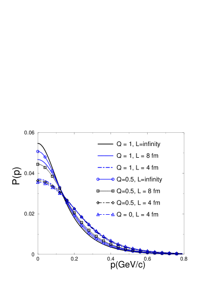
FIG. 1.: (Color online) The normalized spectrum (in arbitrary units) vs. momentum $|$p$|$ (in GeV/c) is shown. The input temperature is $T=0.14$ GeV and the chemical potential is $\mu=0$. The solid line corresponds to the modified Bose-Einstein distribution, i.e., to the limit $R\rightarrow\infty$. The dotted and dashed lines correspond, respectively, to $L=8$ fm and $L=4$ fm. The thicker lines refer to $Q=1.0$ and the thinner ones to $Q=0.5$.

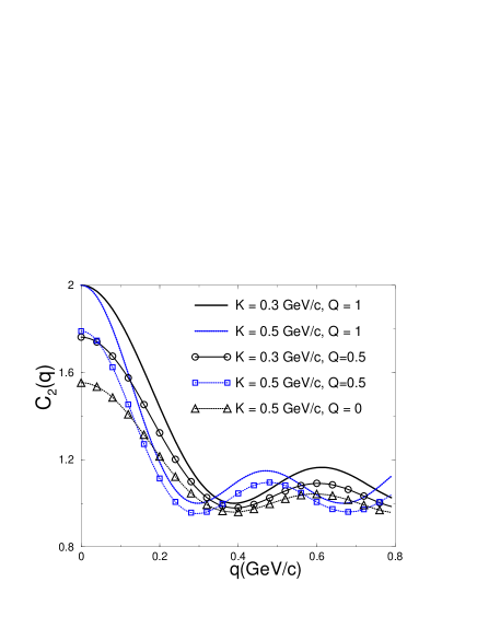
FIG. 2.: (Color online) Two-pion correlation vs. momentum difference $|$q$|$ (in GeV/c). The input temperature is $T=0.14$ GeV and the chemical potential is $\mu=0$. The solid line corresponds to mean momentum $K=0.3$ GeV/c and dashed one to $K=0.5$ GeV/c. The thicker lines refer to the case of $Q=1.0$ and the thinner one to $Q=0.5$. The box size is $L=4$ fm.

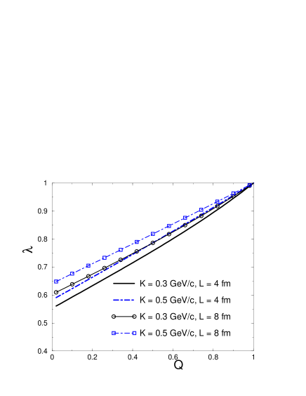
FIG. 3.: (Color online) The intercept parameter, $\lambda$, is shown vs. $Q$, the deformation parameter. The input temperature is $T=0.14$ GeV and the chemical potential is $\mu=0$. The solid line corresponds to mean momentum $K=0.3$ GeV/c and dashed one to the case $K=0.5$ GeV/c. The thicker lines refer to the case $L=4$ fm and the thinner ones to $L=8$ fm.

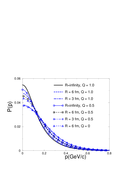
FIG. 4.: (Color online) The normalized spectrum (in arbitrary units) vs. momentum $|$p$|$ (in GeV/c) is shown. The input temperature is $T=0.12$ GeV and the chemical potential is $\mu=0$. The solid line corresponds to the case $R=3$ fm, the dotted one to the case $R=6$ fm, and the dashed line corresponds to the case, $R=\infty$. The thicker lines refer to $Q=1.0$ and the thinner ones to$Q=0.5$.

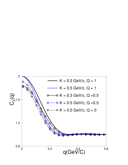
FIG. 5.: (Color online) Two-pion correlation vs. momentum difference $|{\bf q}|$ (in GeV/c) is shown. The input temperature is $T=0.12$ GeV and the chemical potential is $\mu=0$. The solid line corresponds to mean momentum $K=0.3$ GeV/c and the dashed one, to the case $K=0.5$ GeV/c. The thicker lines refer to the case of $Q=1.0$ and the thinner ones to $Q=0.5$. The sphere size is $R=3$ fm.

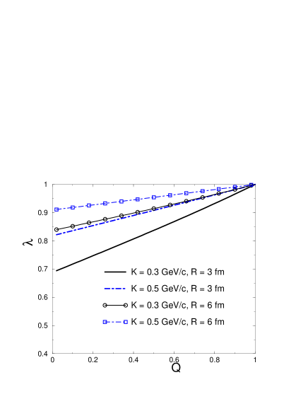
FIG. 6.: (Color online) The intercept parameter, $\lambda$, is shown vs. the deformation $Q$. The input temperature is $T=0.12$ GeV and the chemical potential is $\mu=0$. The solid line corresponds to mean momentum $K=0.3$ GeV/c and dashed one to the case $K=0.5$ GeV/c. The thicker lines refer to the case $R=3$ fm and the thinner ones to $R=6$ fm.

APPENDIX I

We here analyze the $Q=0$ limit in more detail. We can see its implications on the expectation values, directly from Eq.(21)-(22), on the correlation function, from Eq.(45), and on the intercept parameter, $\lambda$, from Eq.(51), by simply imposing the limit $Q=0$. Alternatively, we can start with our definitions in Eq.(13), and thus simultaneously test our results. Lets also go back to the definition in Eq.(20). For Q=0 we see that

$$[n]=\;\;\left\{\begin{array}[]{l}\mbox{ 1 $\rightarrow$ $n\neq 0$}\\ \mbox{ 0 $\rightarrow$ $n=0$}\end{array}\right\}\;.$$ (89)

Thus, $[n]!=1$ in both the above cases. Consequently, instead of Eq.(20), we have

$$|n\rangle_{{}_{l}}=(a_{\l}^{\dagger})^{n}|0\rangle\;.$$ (90)

If we apply to the above equation the annihilation and creation operators, we have

$$a_{\l}|n\rangle_{{}_{l}}=a_{\l}(a_{\l}^{\dagger})^{n}|0\rangle=|n-1\rangle\;;\;a_{\l}^{\dagger}|n\rangle_{{}_{l}}=|n+1\rangle\;,$$ (91)

which follow from the first commutation relations in Eq. (13) and from the condition $a_{\l}|0\rangle=0$. The other commutation relations remain unchanged in this limit.

Let us now estimate the trace of the density matrix, $tr(\rho_{l})$. From Eq.(16) and (17), we have

$$tr(\rho_{l}) = \sum_{n}{{}_{{}_{l}}\!\langle}n|\rho_{l}|n\rangle_{{}_{l}}=\sum_{n=0}^{\infty}\sum_{m=0}^{\infty}[-\frac{1}{T}(E_{l}-\mu)n]^{m}\frac{1}{m!}=$$ (92)

$$= \sum_{n=0}^{\infty}e^{-\frac{1}{T}(E_{l}-\mu)n}=\frac{1}{1-\exp[-\frac{1}{T}(E_{l}-\mu)]}\;\;.$$ (93)

For estimating the limits of Eq.(21) and (22) for $Q\rightarrow 0$ along the lines above, we have to estimate the traces $tr(a^{\dagger}_{l}a_{l}\rho_{l})$ and $tr(a^{\dagger}_{l}a^{\dagger}_{l}a_{l}a_{l}\rho_{l})$, as follows

$$tr(a^{\dagger}_{l}a_{l}\rho_{l}) = \sum_{n}{{}_{{}_{l}}\!\langle}n|a^{\dagger}_{l}a_{l}\rho_{l}|n\rangle_{{}_{l}}=$$ (94)

$$= \sum_{n=0}^{\infty}\sum_{m=0}^{\infty}{{}_{{}_{l}}\!\langle}n|a^{\dagger}_{l}a_{l}[-\frac{(E_{l}-\mu)}{T}]^{m}\frac{N_{l}}{m!}|n\rangle_{{}_{l}}=$$ (95)

$$= \sum_{n=1}\sum_{m}[-\frac{1}{T}(E_{l}-\mu)n]^{m}\frac{1}{m!}{{}_{l}}\!\langle n-1|n-1\rangle_{{}_{l}}$$ (96)

$$= \sum_{n=0}e^{-\frac{1}{T}(E_{l}-\mu)n}-1=$$ (97)

$$= \frac{e^{-\frac{1}{T}(E_{l}-\mu)}}{1-\exp[-\frac{1}{T}(E_{l}-\mu)]}\;\;.$$ (98)

$$tr(a^{\dagger}_{l}a^{\dagger}_{l}a_{l}a_{l}\rho_{l})=\sum_{n}{{}_{{}_{l}}\!\langle}n|a^{\dagger}_{l}a^{\dagger}_{l}a_{l}a_{l}\rho_{l}|n\rangle_{{}_{l}}=$$ (99)

$$= \sum_{n=0}^{\infty}\sum_{m=0}^{\infty}{{}_{{}_{l}}\!\langle}n|a^{\dagger}_{l}a^{\dagger}_{l}a_{l}a_{l}[-\frac{1}{T}(E_{l}-\mu)]^{m}\frac{N_{l}}{m!}|n\rangle_{{}_{l}}=$$ (100)

$$= \sum_{n=1}^{\infty}\sum_{m=0}^{\infty}[-\frac{1}{T}(E_{l}-\mu)n]^{m}\frac{1}{m!}{{}_{{}_{l}}\!\langle}n-1|a^{\dagger}_{l}a_{l}|n-1\rangle_{{}_{l}}=$$ (101)

$$= \sum_{n=2}^{\infty}\sum_{m=0}^{\infty}[-\frac{1}{T}(E_{l}-\mu)n]^{m}\frac{1}{m!}{{}_{{}_{l}}\!\langle}n-2|n-2\rangle_{{}_{l}}=$$ (102)

$$= \sum_{n=0}^{\infty}e^{-\frac{1}{T}(E_{l}-\mu)n}-e^{-\frac{1}{T}(E_{l}-\mu)}-1=\frac{e^{-\frac{2}{T}(E_{l}-\mu)]}}{1-e^{-\frac{1}{T}(E_{l}-\mu)}}.$$ (103)

From the above results and our definition in Eq.(18), it follows immediately that

$$\langle a_{l}^{\dagger}a_{l}\rangle=e^{-\frac{1}{T}(E_{l}-\mu)}=N_{l}\;,$$ (105)

and

$$\langle a_{l}^{\dagger}a_{l}^{\dagger}a_{l}a_{l}\rangle=e^{-\frac{2}{T}(E_{l}-\mu)}\;.$$ (106)

It is then straightforward to conclude that both results coincide with the ones in Eq.(21) and (22), reinforcing the correctness of our results.

The purpose of the above derivation goes beyond what we have just discussed, it is also helpful for discussing more deeply the peculiar limit of $Q\rightarrow 0$. As we have already pointed out in the body of the manuscript, we recover the expected classical result in that limit for single modes only. In other words, only for single modes we have, for $q=p_{1}-p_{2}=0$ (and, consequently, $K=p_{1}=p_{2}$)

$$\lim_{Q\rightarrow 0}C_{2}(K,K)=2\;\;\;;\;\;\;\lim_{Q\rightarrow 0}\lambda(K)=0.$$

In this case, we also recover the well-known form of the Wigner function, i.e.

$$\lim_{Q\rightarrow 0}g_{l}({\bf x},{\bf K})=g({\bf x},{\bf K})g({\bf y},{\bf K}).$$

Nevertheless, when multi-modes are taken into account, the behavior of the above quantities change considerably. For better illustrating this fact, it is convenient to adopt a specific example. Let us choose our toy model in section III.A, for simplicity, restricting ourselves to the $Q=0$ case. In general, $\lambda=\lambda(q=p_{1}-p_{2}=0)=\lambda(K=p_{1}=p_{2})$ but, for simplifying our analytical study, we restrict our analysis to $\lambda(K=0)$. In this case, we see that the square modulus of the wave-function in momentum space can be written as

$$|\tilde{\psi}_{k}(0)|^{2}=\frac{2\sin^{2}(kL/2)}{\pi Lk^{2}}[1-\cos(kL)];kL=n\pi(n=1,2...),$$ (107)

from which we see that only odd values of $n$, i.e., $n=2m-1$ can contribute, resulting in

$$|\tilde{\psi}_{k}(0)|^{2}=\left\{\begin{array}[]{l}\mbox{ $\frac{4L}{(2m-1)^{2}\pi^{3}}$ (m=1,2,...)}\\ \mbox{ }\\ \mbox{ ~{} 0 ~{}(n even)}\end{array}\right.$$ (111)

Then, for writing the chaoticity parameter in the limit of $Q=0$ for the toy model, we rewrite Eq.(51) for this particular case, as

$$\lambda({\bf K})=1-\frac{\sum_{l}\;N_{l}^{2}\;|\tilde{\psi}_{l}({\bf K})|^{4}}{(\sum_{l}N_{l}|\tilde{\psi}_{l}({\bf K})|^{2})(\sum_{l}N_{l}|\tilde{\psi}_{l}({\bf K})|^{2})}\;.$$ (112)

We have then to estimate the sums separately, as follows

$$\sum_{l}N_{l}|\tilde{\psi}_{l}({\bf K})|^{2}=\sum_{l}e^{-\frac{E_{l}}{T}}|\tilde{\psi}_{l}({\bf K})|^{2}\;.$$ (113)

$$\sum_{l}\;N_{l}^{2}\;|\tilde{\psi}_{l}({\bf K})|^{4}=\sum_{l}\;e^{-\frac{2E_{l}}{T}}\;|\tilde{\psi}_{l}({\bf K})|^{4}\;.$$ (114)

For estimating the above sums, it is more convenient to consider appropriate limits for the size of the 1-dimensional box. Let us first assume the limit of very small sizes, i.e., $L\rightarrow 0$. In this case, $E_{l}\approx n\pi/L$, we denote as

$$\left\{\begin{array}[]{l}\mbox{$x=e^{-\frac{E_{1}}{T}}\ll 1$ ($n=1$)}\\ \mbox{ }\\ \mbox{$E_{2m-1}=(2m-1)\pi/L=(2m-1)E_{1}$}\end{array}\right\}\Rightarrow$$ (118)

$$N_{2m-1}=x^{2m-1}$$ (119)

Consequently, the sums for ${\bf K}=0$ can be written as

$$\sum_{m}N_{m}|\tilde{\psi}_{m}({\bf 0})|^{2} = \sum_{m}x^{2m-1}\frac{4L}{\pi^{3}}\frac{1}{(2m-1)^{2}}=$$ (120)

$$= \frac{4L}{\pi^{3}}\sum_{m}\frac{x^{2m-1}}{(2m-1)^{2}}\;.$$ (121)

$$\sum_{m}\;N_{2m-1}^{2}\;|\tilde{\psi}_{2m-1}(0)|^{4} = \sum_{m}\;x^{2(2m-1)}\;\frac{16L^{2}}{(2m-1)^{4}\pi^{6}}=$$ (122)

$$= \frac{16L^{2}}{\pi^{6}}\sum_{m}\frac{x^{2(2m-1)}}{(2m-1)^{4}}\;.$$ (123)

If we then bring Eq.(121) and Eq. (123) into Eq. (112), we get

$$\lim_{L\rightarrow 0(x\rightarrow 0)}\lambda({\bf K=0})=1-\frac{\sum_{m}\frac{x^{2(2m-1)}}{(2m-1)^{4}}}{\left\{\sum_{m}\frac{x^{2m-1}}{(2m-1)^{2}}\right\}^{2}}=$$ (124)

$$= 1-\lim_{L\rightarrow 0(x\rightarrow 0)}\frac{x^{2}(1+\frac{x^{4}}{3^{4}}+\frac{x^{8}}{5^{4}}+\frac{x^{12}}{7^{4}}+...)}{x^{2}(1+2\frac{x^{2}}{3^{2}}+\frac{x^{4}}{3^{4}}+2\frac{x^{4}}{5^{2}}+...)}=1-1=0,$$ (125)

and thus, the expected limit for classical particles is recovered for $Q=0$, when $L\rightarrow 0$.

In the opposite limit of $L\rightarrow\infty$, however, we can see that $k=(2m-1)\pi/L\rightarrow 0$, which implies that $E_{k}\rightarrow m_{\pi}$. Consequently, $N_{k}\rightarrow N_{0}$ = const. In this case

$$\lim_{L\rightarrow 0(x\rightarrow 0)}\lambda({\bf K=0}) = 1-\frac{\sum_{m}\frac{N_{0}^{2}16L^{2}}{\pi^{6}(2m-1)^{4}}}{\left\{\sum_{m}\frac{N_{0}4L}{\pi^{3}(2m-1)^{2}}\right\}^{2}}=$$ (127)

$$= 1-\frac{\frac{\pi^{4}}{96}}{\left\{\frac{\pi^{2}}{8}\right\}^{2}}=1-\frac{2}{3}=\frac{1}{3}\;.$$ (128)

From the result in Eq.(LABEL:chaotoy2) we see that, for the particular density matrix we chose in Eq.(17), the intercept parameter, $\lambda({\bf K}=0)$, can still have the expected value for bosonic interferometry in the classical limit, i.e., $\lambda({\bf K}=0)=0$, even for multi-modes, due to the combined effects of the density of states, $N_{k}$, and of the wave-functions, $\tilde{\psi}_{l}({\bf K}=0)$. However, in the second case, we see from Eq.(128), that $\lim_{L\rightarrow\infty}\lambda({\bf K}=0)=1/3$. This is reflecting the relation between $L$ and $k$ coming from the shape of the wave function and boundary conditions in a finite system, as in Eq.(107). Moreover, the difference among the two limits reflects the particular choice of the density matrix. In order to demonstrate this, we choose a much simpler example than in Eq.(17). For instance, let us choose $\rho_{k}=$ const., and proceed analogously as before. In this case, instead of Eq.(105) and (106), we would have

$$\langle a_{l}^{\dagger}a_{l}\rangle=1=N_{l}\;\;;\;\;\langle a_{l}^{\dagger}a_{l}^{\dagger}a_{l}a_{l}\rangle=1\;,$$ (129)

As a consequence, we get for the sums in Eq.(113), (114) and Eq.(128)

$$\left\{\begin{array}[]{l}\mbox{ $\sum_{l}|\tilde{\psi}_{l}(0)|^{2}=\frac{4L}{\pi^{3}}$ }\\ \mbox{ }\\ \mbox{ $\sum_{l}|\tilde{\psi}_{l}(0)|^{4}=\frac{16L^{2}}{\pi^{6}}$ }\end{array}\right\}\Rightarrow$$ (133)

$$\;\;\lambda({\bf K=0})=1-\frac{\frac{16N_{0}^{2}L^{2}\pi^{4}}{96\pi^{6}}}{\left\{\frac{4N_{0}L\pi^{2}}{8\pi^{3}}\right\}^{2}}=1-\frac{2}{3}=\frac{1}{3}$$ (134)

From what we just saw above, we could say that, if we choose a different type of density matrix, i.e., $\rho_{k}$ = const., for instance, the wave function does not seem to play any role, since we get $N_{k}$=const. Consequently, for this much simpler density matrix, we see that we get $\lambda\rightarrow 1/3$, independently on the energy of the states, $E_{k}$, and on the size of the 1-dimensional box, $L$.

APPENDIX II

For completeness, we will also derive below the so-called type-B $Q$-boson interferometry formulation, as defined in Ref.[17]. For type-B $Q$-boson, the operators $b_{i}$ and $b_{j}$ satisfy the following commutation relations

$$b_{l}b_{l^{\prime}}^{\dagger}-Q^{\delta_{l,l^{\prime}}}b_{l^{\prime}}^{\dagger}b_{l}=\delta_{l,l^{\prime}}Q^{-N_{l}}$$ (135)

$$b_{l}b_{l^{\prime}}^{\dagger}-Q^{-\delta_{l,l^{\prime}}}b_{l^{\prime}}^{\dagger}b_{l}=\delta_{l,l^{\prime}}Q^{N_{l}}$$ (136)

$$[b_{l},b_{l^{\prime}}]=[b_{l}^{\dagger},b_{l^{\prime}}^{\dagger}]=0,$$ (137)

$$[\hat{N}_{l},b_{l^{\prime}}]=-\delta_{l,l^{\prime}}b_{l}$$ (138)

$$[\hat{N}_{l},b_{l^{\prime}}^{\dagger}]=\delta_{l,l^{\prime}}b_{l}^{\dagger},$$ (139)

$$[\hat{N}_{l},\hat{N}_{l^{\prime}}]=0.$$ (140)

In the above relations $Q$ is a parameter, which can be assumed within $[-1,1]$. If we define it, following Ref.[17], as $Q=e^{i\theta}$ ($0\leq\theta<2\pi$) or, equivalently, $\cos(\theta)=\frac{1}{2}(Q+Q^{-1})$, then

$$\langle b_{l}^{\dagger}b_{l}\rangle=$$ (141)

$$= \frac{\exp(\frac{1}{T}(E_{l}-\mu))-1.}{\exp(\frac{2}{T}(E_{l}-\mu))-2\cos(\theta)\exp(\frac{1}{T}(E_{l}-\mu)+1}=$$ (142)

$$= \frac{\exp[\frac{-1}{2T}(E_{l}-\mu)]\sinh[\frac{1}{2T}(E_{l}-\mu)]}{\cosh[\frac{1}{T}(E_{l}-\mu)]-\cos(\theta)}$$ (143)

and

$$\langle b_{l}^{\dagger}b_{l}^{\dagger}b_{l}b_{l}\rangle=$$ (144)

$$= \frac{2\cos(\theta)}{\exp(\frac{2}{T}(E_{l}-\mu))-2\cos(2\theta)\exp(\frac{1}{T}(E_{l}-\mu)+1}$$ (145)

$$= \frac{\cos(\theta)\exp[\frac{-1}{T}(E_{l}-\mu)]}{\cosh[\frac{1}{T}(E_{l}-\mu)]-\cos(2\theta)}\;.$$ (146)

As before, the expectation value $\langle\hat{b}^{\dagger}_{l}\hat{b}_{l^{\prime}}\rangle$ is related to the occupation probability of the single-particle state $l$, $N^{(b)}_{l}$, by a similar relation, i.e.,

$$\langle\hat{b}^{\dagger}_{l}\hat{b}_{l^{\prime}}\rangle=\delta_{l,l^{\prime}}N^{(b)}_{l}\;\;.$$ (147)

Then similar to the derivation of Eq.(16) and Eq.(20),we have

$$P_{1}({\bf p})=\sum_{l}\langle b_{l}^{\dagger}b_{l}\rangle\tilde{\psi}_{l}^{*}({\bf p})\tilde{\psi}_{l}({\bf p})$$ (148)

and

$$P_{2}({\bf p_{1},p_{2}})=P_{1}({\bf p_{1}})P_{1}({\bf p_{2}})+|\sum_{l}\tilde{\psi}_{l}^{*}({\bf p_{1}})\tilde{\psi}_{l}({\bf p_{2}})|^{2}$$ (149)

$$+\sum_{l}\tilde{\psi}_{l}^{*}({\bf p_{1}})\tilde{\psi}_{l}^{*}({\bf p_{2}})\tilde{\psi}_{l}({\bf p_{1}})\tilde{\psi}_{l}({\bf p_{2}})[\langle b_{l}^{\dagger}b_{l}^{\dagger}b_{l}b_{l}\rangle-2\langle b_{l}^{\dagger}b_{l}\rangle]$$ (150)

$$=P_{1}({\bf p_{1}})P_{1}({\bf p_{2}})\!+\!\sum_{l,l^{\prime}}\ N_{l}N_{l^{\prime}}\!\!\tilde{\psi}_{l}^{*}({\bf p_{1}})\tilde{\psi}_{l^{\prime}}^{*}({\bf p_{2}})\tilde{\psi}_{l}({\bf p_{2}})\tilde{\psi}_{l^{\prime}}({\bf p_{1}})$$ (151)

$$\!\!\left\{1-\delta_{l,l^{\prime}}(1-\cos\theta)\!\!\left[\frac{4\cosh^{2}(\frac{E_{l}-\mu}{2T})+\frac{\cos\theta(\cos\theta-1)}{\sinh^{2}(\frac{E_{l}-\mu}{2T})}}{\cosh(\frac{E_{l}-\mu}{T})-\cos(2\theta)}\right]\right\}\!.\!$$ (152)

Analogously to what was done at the end of Section II, we can also define a modified Wigner function for type-B $Q$-boson. The new Wigner function for this case can be defined similarly as before, resulting in

$$g^{(b)}({\bf x},{\bf K};{\bf y},{\bf K})=g^{(b)}({\bf x},{\bf K})g^{(b)}({\bf y},{\bf K})-$$ (153)

$$\!\sum_{l}\!\left\{\!(N^{(b)}_{l})^{2}(1-\cos\theta)\left[\!\frac{\!4\cosh^{2}(\frac{E_{l}-\mu}{2T})+\frac{\cos\theta(\cos\theta-1)}{\sinh^{2}(\frac{E_{l}-\mu}{2T})}\!}{\cosh(\frac{E_{l}-\mu}{T})-\cos(2\theta)}\!\right]\!\!\right\}\!.\!\!$$ (154)

Then the two-pion interferometry formula follows analogously to Eq.(62) for this case, i.e.,

$$C_{2}^{(b)}({\bf p_{1},p_{2}})=1+\frac{\int\int e^{-i{\bf q}.({\bf x}-{\bf y})}g^{(b)}({\bf x},{\bf K};{\bf y},{\bf K})d{\bf x}d{\bf y}}{\int g^{(b)}({\bf x},{\bf p_{1}})d{\bf x}\int g^{(b)}({\bf y},{\bf p_{2}})d{\bf y}}$$ (155)

REFERENCES

- [1] See for example: C.Y. Wong, Introduction to high energy heavy-ion collisions, (World Scientific, Singapore, 1994); Quark-Gluon-Plasma 2, edited by R.C. Hwa ( World Scientific, Singapore, 1995).
- [2] Proceedings of Quark Matter 2001, January 14-20, SUNY, USA, Nucl. Phys. A 698 (2002); Proceedings of Quark Matter 2002, July 18-24, Nantes, France, Nucl. Phys. A 715 (2003).
- [3] R. Hanbury-Brown and R.Q. Twiss, Phil. Mag. 45, 663 (1954); Nature 177, 27 (1956) and 178, 1447 (1956).
- [4] G. Goldhaber, S. Goldhaber, W. Lee, and A. Pais, Phys. Rev. 120, 300 (1960).
- [5] for a long list of references on interferometry, see i) W.A. Zajc, Il Ciocco 1992, Particle production in highly excited matter (NATO Advanced Study Institute), p. 435, Castelvecchio Pascoli, Italy, 12-24 Jul 1992; ii) D. H. Boal, C. K. Gelbke, and B. K. Jennings, Rev. Mod. Phys. 62, 553 (1990); iii) R. M. Weiner, Bose-Einstein Correlation in Particle and Nuclear Physics, J. Wiley & Sons (1997); iv) U. Heinz and B. V. Jacak, Ann. Rev. Nucl. Part. Sci. 49, 529 (1999).
- [6] Q. H. Zhang and Sandra S. Padula, Phys. Rev. C 62 024902 (2000).
- [7] E. V. Shuryak, Phys. Rev. D 42, 1764 (1990).
- [8] C.Y. Wong, Phys. Rev. C 48, 902 (1993).
- [9] Yu. Sinyukov, Nucl. Phys. A566, 589c (1994).
- [10] M. G.-H. Mostafa and C.Y. Wong, Phys. Rev. C 51, 2135 (1995).
- [11] A. Ayala and A. Smerzi, Phys. Lett. B405, 20 (1997); A. Ayala, J. Barreiro and L. M. Montaño, Phys. Rev. C 60, 014904 (1999).
- [12] S. Sarkar, P. K. Roy, D. K. Srivastava, and B. Sinha, J. Phys. G22, 951 (1996).
- [13] O.W. Greenberg, Phys. Rev. Lett. 64, 705 (1990), and Phys. Rev. D43, 4111 (1991).
- [14] D.D. Coon, S. Yu and M. Baker, Phys. Rev. D5, 1429 (1972); P. Kulish and E. Damaskinsky, J. Phys. A 23, L 415 (1990); S. Chaturvedi, A. K. Kapoor, R. Sandhya, V. Srinivasan and R. Simon, Phys. Rev. A 43, 4555 (1991)
- [15] D. V. Anchishkin, A. M. Gavrilik, and S. Y. Panitkin, hep-ph/0112262.
- [16] S. S. Avancini and G. Krein, J. Phys. A: Math. Gen. 28, 685 (1995).
- [17] D. V. Anchishkin, A. M. Gavrilik and N. Z. Iorgov, Eur. Phys. J. A7 229 (2000); Mod. Phys. Lett A15 (2000) 1637.
- [18] S. Pratt, Phys. Rev. Lett. 53, 1219 (1984).
- [19] S. S. Padula, M. Gyulassy, and S. Gavin, Nucl. Phys. B329, 357 (1990).
- [20] W. Q. Chao, C. S. Gao and Q. H. Zhang, Phys. Rev. C49, 3224 (1994).
- [21] O. V. Utyuzh, G. Wilk, M. Rybczyński, and Z. Wlodarczyk, hep-ph/0210328.
- [22] Urs Wiedemann and U. Heinz, Phys. Rept. 318, 145 (1999).
- [23] T. Csorgo, hep-ph/0001233.
- [24] A. Ayala and A. Sanchez, Phys. Rev. C63, 064901 (2001).